High frequency and high wavenumber solar oscillations

Abstract

We determine the frequencies of solar oscillations covering a wide range of degree ($100<\ell<4000$) and frequency ($1.5<\nu<10$ mHz) using the ring diagram technique applied to power spectra obtained from MDI (Michelson Doppler Imager) data. The f-mode ridge extends up to $\ell\approx 3000$, where the line width becomes very large, implying a damping time which is comparable to the time period. The frequencies of high degree f-modes are significantly different from those given by the simple dispersion relation $\omega^{2}=gk$. The f-mode peaks in power spectra are distinctly asymmetric and use of asymmetric profile increases the fitted frequency bringing them closer to the frequencies computed for a solar model.

1 Introduction

It is well known that solar acoustic modes with frequencies less than the acoustic cut-off frequency of the photosphere ($\approx 5.3$ mHz) are trapped below the solar photosphere. These modes have been successfully used to probe the internal structure and dynamics of the Sun. At higher frequencies the modes are expected to propagate into the chromosphere, where they are likely to be damped due to radiative dissipation. Nevertheless, a number of observations (cf., Duvall et al. 1991; Fernandes et al. 1992; Kneer & von Uexküll 1993) have conclusively established that the p-mode ridges continue well beyond the estimated acoustic cut-off frequency in the solar photosphere. Various mechanisms have been put forward to explain the observed high frequency p-modes. Balmforth & Gough (1990) suggested that the high frequency modes may arise due to the reflection of waves at the transition layer between the chromosphere and corona, where the temperature and hence the sound speed rises rapidly. In that case we would also expect to observe the chromospheric modes trapped in the chromospheric cavity (Ulrich & Rhodes 1977; Ando & Osaki 1977) expected to be formed around the temperature minimum. Despite several attempts, there has not been any unambiguous detection of the chromospheric modes (Duvall et al. 1991; Fernandes et al. 1992; Kneer & von Uexküll 1993), and hence Kumar & Lu (1991) suggested that the high frequency modes arise from interference between two traveling acoustic waves. It has been argued that because of inhomogeneities in the structure of the chromosphere corona transition layer the chromospheric cavity may not be sufficiently well defined to support resonant modes (Kumar 1993).

Apart from the p-modes, f-modes have also been detected at high degrees. These high degree f-modes are expected to be localized in the chromosphere and hence can provide a diagnostic for velocity fields prevailing there. The frequencies of these modes are expected to be essentially independent of the stratification in solar interior and hence the difference between the observed frequencies (cf., Libbrecht, Woodard, & Kaufman 1990; Bachmann et al. 1995; Duvall, Kosovichev & Murawski 1998) and those of solar models have been interpreted to be due to velocity field or magnetic fields and other effects (cf., Campbell & Roberts 1989; Murawski & Roberts 1993; Rosenthal & Gough 1994). Although, Fernandes et al. (1992) have measured the frequencies of f-modes up to $\ell\approx 3700$, the accuracy of these frequencies is limited due to the short duration of their observations (2.4 hrs). Similarly, using 8 hrs of observations, Duvall et al. (1998) have calculated the frequencies of f-modes up to $\ell\approx 1800$ and they have interpreted the decrease in observed frequency as compared to model frequency as arising due to turbulent velocity fields. It would thus be interesting to check the frequencies of these modes at higher degree as these are expected to be localized in the chromosphere.

The frequencies of these modes have been calculated by fitting a symmetric Lorentzian profile to the power spectra. It has been demonstrated that in general the peaks in power spectra are not symmetric (Duvall et al. 1993; Toutain 1993; Nigam & Kosovichev 1998; Toutain et al. 1998) and the use of symmetric profiles may cause the fitted frequency to be shifted away from the true value. Thus, it would be interesting to estimate the frequencies using fits to asymmetric profiles.

In this work we use the data obtained by Michelson Doppler Imager (MDI) on board the Solar and Heliospheric Observatory (SOHO) to measure frequencies of f and p-modes at high degrees. We have examined power spectra that extend up to degree $\ell\approx 5000$ and frequency $\nu\approx 16$ mHz, to identify oscillatory modes with degrees up to $\ell=4000$ and frequencies up to $\nu=10$ mHz. Beyond these limits there is too little power to fit the modes reliably. The rest of the paper is organized as follows: we describe the observations and analysis technique in Section 2, while the results are described in Section 3. Finally, we summarize the main conclusions from our study in Section 4.

2 The technique

We adopt the ring diagram technique (Hill 1988; Patrón et al. 1995) to determine the mean frequency of solar oscillations at high degree ($\ell>100$) (cf., Fernandes et al. 1992). We use MDI data and the MDI data-analysis pipe-line to obtain three dimensional (3d) power spectra of solar oscillations as described by Basu, Antia & Tripathy (1999). However unlike Basu et al. (1999) we have not applied any temporal detrending to the time series since that produces a broad peak at the frequency corresponding to that of the detrending interval.

We have used both full-disk and high-resolution Dopplergrams produced by MDI. Full-disk Dopplergrams give the power spectra for modes with degree up to $1500$, while high-resolution Dopplergrams can produce spectra for modes with degrees up to $5000$. These observations are taken at a cadence of 1 minute thus giving a Nyquist limit of 8.33 mHz. From the available full-disk Dopplergrams we have selected 24 intervals of 1536 minutes each covering a period from May 25 to June 21, 1996. These correspond to longitudes centered at 90, 76, 60, 45, 30 and 15 degrees for Carrington rotation 1909, and longitudes 360, 345, 330, 315, 300, 285, 270, 255, 240, 225, 210, 195, 181, 160, 150, 135, 120 and 105 degrees for Carrington rotation 1910. The slightly uneven distribution in the longitudes is due to our attempt to avoid data gaps. For each time series we have selected three regions centered at the central meridian and at latitudes of $0,\pm 15^{\circ}$, covering $256\times 256$ pixels in longitude and latitude. We have summed all 72 spectra to improve statistics. These summed spectra effectively cover a time interval of 26 days, which improves the statistics.

For the spectra obtained from high-resolution Dopplergrams we have taken the sum over 24 spectra covering the available data for March 1997 and from June to July 1997. The longitude and latitude distribution of the data used was determined by the availability of observed images. We used time series of $256\times 256$ pixel images centered at a latitude of 11^∘ N and longitudes of 200 and 185 degrees for Carrington rotation 1920, at latitudes of 11^∘ N and 18^∘ N for longitudes 50, 35, 20 and 5 degrees for Carrington rotation 1923, and for longitudes 135, 120, 105, 90, 75, 60 and 45 degrees for Carrington rotation 1924. Although we tried to select periods with least data-gaps, nevertheless the high-resolution data sets have many more gaps than the full-disk set and this affects the quality of the resulting spectra. Since the high-resolution Dopplergrams do not cover the entire solar disk there could be some error in estimating the spatial scale, which has been obtained from the relevant parameters in the image headers. The difference in frequencies obtained from the two spectra would give an estimate of such systematic errors. We have also used full-disk Dopplergrams taken at higher cadence of 30 s to study higher frequency modes that extend to 16 mHz. For this purpose we have summed over 24 spectra, each obtained from time series of 1024 minutes, covering the available data for June 1997.

These summed 3d spectra are averaged in the azimuthal direction to obtain 2d (two dimensional) spectra in $k$ and $\nu$, where $k$ is the horizontal wavenumber. For the full-disk spectra the Nyquist limit on individual spatial components $k_{x}$ and $k_{y}$ corresponds to $\ell\approx 1500$. However, while taking the azimuthal averages we can extend the spectra to about $\ell=2100$ (the maximum value of $k=\sqrt{k_{x}^{2}+k_{y}^{2}}$) by averaging over partial and incomplete rings too at fixed temporal frequency. This can introduce some systematic errors for $\ell>1500$ because of spatial aliasing and averaging over only a part of ring. However, comparison with results obtained using the high-resolution Dopplergrams shows that this effect is not very significant.

We fit the sections at constant $k$ (or $\ell$) in the averaged spectra to a Lorentzian profile of the form,

$$P(\ell,\nu)={\exp{A_{0}}\over(\nu-\nu_{0})^{2}+w_{0}^{2}}+e^{b_{1}}[1+b_{2}(1-\nu/\nu_{c})],$$ (1)

where the 5 parameters $A_{0},\nu_{0},w_{0},b_{1}$ and $b_{2}$ are determined by fitting the spectra using a maximum likelihood approach (Anderson, Duvall & Jefferies 1990). Here $\nu_{c}$ is the central value of $\nu$ in the fitting interval, $\nu_{0}$ is the fitted frequency and $w_{0}$ is the half-width. The peak power in the mode is given by $\exp(A_{0})/w_{0}^{2}$. The terms involving $b_{1}$ and $b_{2}$ define the background power. We generally fit each peak in the spectra separately by fitting a region extending roughly half way to the adjoining peaks. In order to check the sensitivity of fits to the presence of neighboring peaks we also fit two or three neighboring modes simultaneously. We find that these independent fits give results which agree with each other to within the estimated errors. We examine each of the fits visually to reject all those cases where the program fitted stray noise spikes in the power spectra. Apart from this, we also fit the 3d spectra directly as described by Basu et al. (1999). We find that these frequencies also agree with those determined from averaged 2d spectra. For the full-disk spectra we have also fitted the sum of the 24 spectra centered at the equator (and $\pm 15^{\circ}$ latitude) and these frequencies also agree with those calculated from the sum over all 72 spectra. Thus it is clear that the fitted frequencies are fairly robust.

3 Results

Fig. 1 shows the $\ell$-$\nu$ diagram for the fitted modes. This includes the results obtained from all three spectra. It is clear that the frequencies computed from the three independent spectra agree with each other as all points appear to fall in the same series of ridges. These frequencies are also in agreement with those determined by Rhodes et al. (1998) from MDI spectra for $\ell<1000$ as well as with those determined by Fernandes et al. (1992). This figure also shows the frequencies computed for two solar models, one without a chromosphere (henceforth called Model 1) and one with a chromosphere (Model 2).

Both Model 1 and Model 2 are static solar models computed using the hydrogen abundance profile inferred from helioseismic data (Antia & Chitre 1998) and heavy element abundance profile from model 5 of Richard et al. (1996). These models use OPAL opacity tables (Iglesias & Rogers 1996), OPAL Equation of state (Rogers, Swenson & Iglesias 1996) and nuclear reaction rates as adopted by Bahcall & Pinsonneault (1995). We use the formulation of Canuto & Mazzitelli (1991) to calculate the convective flux. Thus both models are identical in the interior, but Model 1 extends only up to the temperature minimum, while Model 2 includes a chromosphere. For the chromospheric region in Model 2 we use Model C of Vernazza, Avrett & Loeser (1981).

The frequencies for these solar models are computed using the usual adiabatic equation, neglecting all dissipative effects. For Model 1, the outer boundary conditions for calculating the frequencies are applied at the temperature minimum, for Model 2, they are applied in the chromosphere corona transition layer at a height of 2300 km above the solar surface. The frequencies of Model 1 (no chromosphere) show the normal f- and p-mode ridges. For Model 2, which has a chromosphere, we get a series of avoided crossings between these p-mode ridges, corresponding to each chromospheric mode (cf., Ulrich & Rhodes 1977). In addition we also get a series of chromospheric g-modes for this model.

We show the width of the fitted modes in Fig. 2. The figure also shows the locus of points where the damping time ($1/2\pi w_{0}$) equals the period of oscillatory mode. The width for f- and $p_{1}$-modes with $\ell<1800$ agrees reasonably with the values obtained by Duvall et al. (1998). It may be noted that the half-width of p-modes appears to reach a constant value of about 0.2 mHz at high frequencies ($\nu>6$ mHz). The corresponding life-time for these modes is comparable to the wave travel time from surface to lower turning point and back (cf., Duvall et al. 1991). Most of the scatter seen in Fig. 2 at high frequencies is due to statistical errors in estimating these widths. From the figure it appears that at low frequencies the width increases with decreasing frequencies. We believe that this is artificial and due to the fact that the width is actually less than the resolution limit of our spectra. We have tried fits keeping the width fixed for these modes to check that the fitted frequencies are not affected by this behavior.

Fig. 3 shows the power spectra for $\ell=1295$ obtained using the full-disk Dopplergrams. Apart from the normal f- and p-modes it shows two more peaks at frequencies of about 1.25 and 2.35 mHz and some other peaks between the p-mode peaks. These peaks are not seen in the spectra obtained using high-resolution Dopplergrams and they are believed (Duvall, Hill & Scherrer; private communications), to be due an artifact arising from the fact that tracking the full-disk image with solar rotation rate leads to a shift by one pixel in approximately 800 s, giving a frequency of 1.25 mHz. This frequency then produces side lobes for each of the f- and p-modes giving rise to other peaks with frequencies differing by $\pm 1.25$ mHz from the real peaks.

3.1 The f-mode

As can be seen from Fig. 1, we are able to detect the f-mode ridge up to $\ell\approx 4000$. The f-modes are surface gravity modes and their frequencies are asymptotically expected to satisfy the simple dispersion relation

$$\omega^{2}\approx gk={GM_{\odot}\sqrt{\ell(\ell+1)}\over R_{\odot}^{3}},$$ (2)

where $g$ is the acceleration due to gravity at the surface, $k$ is the horizontal wave number, $G$ is the gravitational constant and $\ell$ the degree of the mode. The f-mode frequencies have previously been determined using different data sets (e.g., Bachmann et al. 1995; Duvall et al. 1998) and some of these results are compared with our measurement in Fig. 4. This figure shows $\omega^{2}/gk$ evaluated at the surface ($r=R_{\odot}$). Theoretically, this ratio is expected to be around unity for f-modes. We find that the frequencies obtained from the full-disk and the high-resolution observations are close to each other, though there is a small systematic difference between the two. This difference could be due to error in estimating the spatial scale in high-resolution Dopplergrams. There is also some systematic difference between frequencies obtained from different observations which should give an estimate of systematic errors that can be expected in these frequencies. All sets of observed frequencies show a similar dip in the curve. For comparison, we also show this ratio for Model 2.

The dip in the curve for the model is due to the fact that for large $\ell$ the f-modes are effectively trapped in the atmosphere where $gk\sim 1/r^{3}$ is smaller than its surface value. This happens because f-modes are characterized by eigenfunctions where the radial velocity $v_{r}$, increases outwards exponentially as $e^{kz}$, where $z$ is the height above the solar surface (Gough 1993). For small $k$, the velocity scale height is much larger than the density scale height in the solar atmosphere and hence the kinetic energy density $\rho v_{r}^{2}$ decreases with height. Thus these modes are localized below the solar surface. But for $\ell\gtrsim 2000$ the kinetic energy density may not decrease with height near the top of convection zone and the peak in kinetic energy density will shift outward towards the chromosphere-corona transition region. However, the minimum value of density scale height in chromospheric models is about 100 km, and hence for f-modes with $\ell\gtrsim 3500$ the kinetic energy density may keep increasing with height and we would not expect such modes to be observed. In Model 2 we have imposed an artificial boundary at a height of about 2300 km ($0.0033R_{\odot}$), and hence $\omega^{2}$ saturates to $gk$ corresponding to this height. The Sun, however, does not have a well defined boundary and we do not expect this behavior at large $\ell$.

The observed $\omega^{2}/gk$ shows a sharp dip at intermediate values of $\ell=1000-2000$ which Duvall et al. (1998) have interpreted as being due to turbulent velocity fields in the solar convection zone. We find that there is a distinct rise in the ratio $\omega^{2}/gk$ at higher $\ell$ ($\gtrsim 2500$) which is not properly understood. This may be due to the fact that these modes are located in the chromosphere rather than subsurface layers, where the relevant velocity fields will be different.

It can be seen from Fig. 2 that the width for f-modes increases much more rapidly with $\nu$ as compared to the p-modes. Further, the width becomes very large by $\ell\approx 3000$ ($\nu\approx 5.35$ mHz) and the corresponding damping time ($1/2\pi w_{0}$) is comparable to the time-period of the oscillation. Hence beyond this point the mode can not be considered to exist as a normal standing wave. This is expected since beyond this value of $\ell$, the kinetic energy density for f-mode will not decrease with height. The sharp increase in the width of these modes is probably a reflection of that. At even higher degrees, it appears that the width becomes roughly constant with increasing frequency and we believe that the mode is no longer an f-mode. From Fig. 1 it appears that at very high $\ell$ the frequencies of the f-modes tend towards those of the chromospheric modes in Model 2. It may be noted that because of very large half-width ($\approx 1$ mHz) and low power it is not possible to separate the f-mode ridge from the lowest chromospheric mode ridge in this region. It is quite possible that for $\ell\gtrsim 3000$ the f-mode power reduces sharply and hence the corresponding ridge in the observed spectra is dominated by that of the chromospheric mode. This probably explains the sharp increase in $\omega^{2}/gk$ seen in Fig. 4 and also the fact that the width appears to become roughly constant for $\ell\gtrsim 3000$.

3.2 Influence of the chromosphere on p-modes

It appears from Fig. 1 that the frequencies of Model 1 are in remarkable agreement with the observed p-mode ridges. It is possible that this agreement is merely a coincidence where the effect of dissipation has compensated the expected shift from inclusion of chromosphere. To test this we can try to estimate the phase shift associated with reflection of the wave at upper turning point for these modes by fitting the frequencies to the asymptotic form

$${\pi(n+\alpha(\omega))\over\omega}=F\left({\omega\over L}\right),$$ (3)

where $L=\ell+1/2$ and $\alpha(\omega)$ is believed to include the contribution arising from phase shift at outer turning point (cf., Duvall et al. 1991). We have estimated $\alpha(\omega)$ by fitting this form in the frequency interval of 2–8.5 mHz and the results are shown in Fig. 5. It is clear that there is a significant difference between the observed and model frequencies at intermediate frequencies. For observed frequencies $\alpha$ changes rather steeply at intermediate frequencies, which is where the upper turning point for modes shifts from photosphere to chromosphere corona transition region. This is not the case for frequencies of Model 1. Further, for observed frequencies $\alpha$ is almost constant for $\nu\gtrsim 5$ mHz. This can be considered to be an estimate of the acoustic cutoff frequency in the photosphere. Above that frequency all modes propagate in the chromosphere, as a result these modes suffer roughly the same phase shift at the upper turning point which should be located in the chromosphere corona transition layer.

Fig. 6 shows the frequency separation between adjacent modes of the same degree. For observed frequencies $(\nu_{n+1,\ell}-\nu_{n,\ell})$ shows a bump around $\nu=5-6$ mHz. This could be a signature of avoided crossings between these modes, which have not been explicitly seen because of low power in the chromospheric modes. The amplitude of the bump decreases with increasing $n$, which is expected since modes of the same frequency but larger $n$ will penetrate deeper below the surface making the relative effect of chromosphere smaller. The bump also shifts towards lower frequency as $n$ increases, which is to be expected as the frequency of the second chromospheric mode in Model 2 does decrease slowly as $\ell$ reduces (cf., Fig. 1). The frequency separation for Model 1 does not show any such bump. The first chromospheric mode around a frequency of 4 mHz has a relatively sharp avoided crossing, as seen for the theoretical solar model and is not likely to cause any significant bump in the frequency separation. At higher frequencies, the chromospheric cavity merges with the internal cavity and there would be no separate chromospheric modes. Hence we do not expect any more bumps in the frequency separation.

3.3 Effect of asymmetry of the peak profiles

From Fig. 3 it is clear that the profile for f-mode peak is significantly asymmetric with higher power on the lower side of the peak. Hence, fit to a symmetric Lorentzian profile given by Eq. (1) is likely to result in significant shift in the fitted frequencies. In order to get better fit we have also attempted fits using asymmetric profiles of the form (cf., Nigam & Kosovichev 1998)

$$P(\ell,\nu)={e^{A_{0}}[(1+Bx)^{2}+B^{2}]\over 1+x^{2}}+e^{b_{1}}[1+b_{2}(1-\nu/\nu_{c})],$$ (4)

where $x=(\nu-\nu_{0})/w_{0}$ and $B$ is a parameter that controls the asymmetry. This parameter is positive for positive asymmetry, i.e., more power on the higher frequency side of the peak, and negative for negative asymmetry. The parameter $B$ is also fitted along with other parameters defining the line profile. For low order modes ($n=0,1,2$) this parameter is found to be significant, while at higher radial order it is difficult to distinguish between fits with symmetric or asymmetric profiles and the value of $B$ is generally within the corresponding error estimates.

Fig. 7 shows the fits for $\ell=1195$ f-mode using both symmetric and asymmetric profiles. It is clear from this figure that the symmetric profile does not fit the observed power spectrum properly and tends to underestimate the frequency. The asymmetric profile leads to a nearly perfect fit to the observed spectrum and we would expect the corresponding frequency to be more reliable. Since $B$ is negative for all f-modes the frequency shifts to higher value when asymmetric profile is used for fitting.

Fig. 8 shows $\omega^{2}/gk$ for f-mode frequencies obtained using the symmetric and asymmetric profiles. It is clear that use of asymmetric profiles results in frequencies which are significantly higher and the shift in frequencies due to use of asymmetric profiles is much larger than the error estimate in individual fits. Further, the difference between the observed and model frequencies for f-modes is somewhat reduced when asymmetric profiles are used. However, it is clear from the figure that even after accounting for asymmetry in profiles, the observed frequencies around $\ell=2000$ are significantly lower than the frequencies computed for a solar model.

Fig. 9 shows the asymmetry parameter $B$ as obtained from the fits using asymmetric profiles for $n=0,1,2$. It is clear that the value of $B$ is significantly different from zero, which is expected because of clear asymmetry seen in power spectra (Figs. 3, 7). For $p_{2}$-mode at low frequency it is not possible to distinguish between fits to symmetric and asymmetric profiles and the resulting value of $B$ is consistent with zero within the estimated errors. The same is true for higher radial order $n$ and hence these modes are not fitted using asymmetric profiles as the fits with symmetric profiles are found to be more stable. The resulting scaled frequency shift between the asymmetric and symmetric profiles is shown in Fig. 8. The frequency differences are scaled by $Q_{n\ell}$, the ratio of the inertia of the mode to that of a radial mode with the same frequency (Christensen-Dalsgaard & Berthomieu 1991). It appears that to first approximation the scaled frequency shift is a function of frequency alone. The net shift in f-mode frequency is much larger than those in $p_{1}$-mode, but because of difference in $Q_{n\ell}$ the scaled frequency differences are of same order. For f-modes the frequency shift increases with $\ell$ from less than 1 $\mu$Hz at $\ell\approx 250$ to over 100 $\mu$Hz at $\ell\approx 3000$. Further, for p-modes the frequency shifts are comparable to the corresponding error estimates. Nevertheless, the scaled frequency shifts are not exactly a function of frequency alone and hence the correction in frequencies due to asymmetric profile can affect the results of helioseismic inversions to some extent.

4 Conclusions

Using the ring diagram technique applied to MDI data we have determined the frequencies of solar oscillations covering a wide range of degree and frequency. We have improved the quality of the power spectra by taking the sum over several spectra, thus effectively increasing the time duration of observations to about 26 days. The line widths for the high frequency ($\nu>6$ mHz) p-modes appear to be roughly constant, which is to be expected as all these modes have significant amplitude in the chromosphere, where radiative damping is dominant.

The f-mode frequencies at high wavenumbers deviate significantly from those calculated for a solar model. The ratio $\omega^{2}/gk$ for the observed frequencies shows a sharp dip around $\ell=2500$, after which this ratio increases. It appears that the f-mode does not have significant power beyond $\ell=3000$, which is consistent with the fact that the minimum scale height in the solar atmosphere is around 100 km. The damping time estimated from the width of f-mode becomes shorter than the time-period around $\ell=3000$ and the apparent continuation of the ridge at higher degree is probably the lowest chromospheric p-mode.

The f-mode peaks in power spectra are distinctly asymmetric and use of symmetric profiles in fitting the power spectrum results in significant shift in the estimated frequencies. The estimated frequencies increase by up to 100$\mu$Hz, when asymmetric profiles are used in fitting. The frequency shift due to asymmetric profiles reduces at low degree but it may still be significant for $100\leq\ell\leq 250$ which has been studied using global power spectra (Schou et al. 1997; Antia 1998). This may also affect the seismic estimate of solar radius.

Although we do not find any direct evidence for the avoided crossings expected due to chromospheric modes, the frequency difference $\nu_{n+1,\ell}-\nu_{n,\ell}$ has a distinct bump around a frequency of 5–6 mHz, which may be due to avoided crossings. This is the same frequency range where Harvey et al. (1993) and Tripathy & Hill (1995) have observed a broad background feature in the normal p-mode spectra.

Figure 1: The $\ell$–$\nu$ diagram of the modes obtained by our analysis. The crosses display the fitted modes obtained from the full-disk and high-resolution Dopplergrams, including the full-disk observations at higher cadence of 30s. The continuous lines show the modes for Model 2 (i.e., one which has a chromosphere). The dashed lines are the ridges for Model 1, which is truncated at the temperature minimum. The labels near the right and top axis identify some of these ridges.

Figure 2: The half-width of the fitted modes. The squares show the f-modes while the crosses are for the p-modes. The continuous line marks the width for which the damping time is equal to the time-period of oscillation.

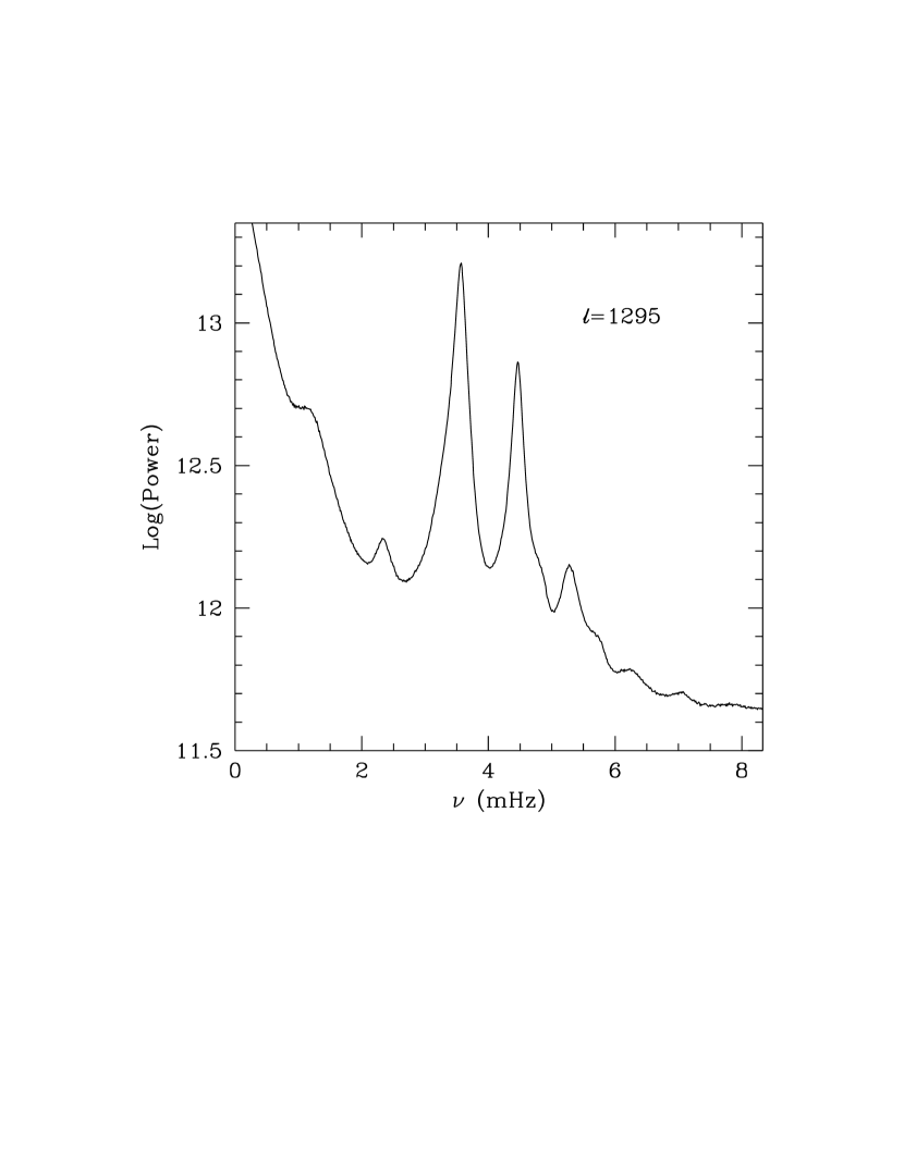
Figure 3: The power spectrum for $\ell=1295$ obtained from full-disk Dopplergrams. The vertical axis is in arbitrary units. The peaks at around 1.25 and 2.35 mHz are artifacts introduced by tracking of images with solar rotation rate.

Figure 4: The ratio $\omega^{2}/gk$ for various observed frequencies of f-modes are displayed. The crosses are data from Bachmann et al. (1995). the triangles are from MDI data (Rhodes et al. 1997; Duvall et al. 1998). The continuous line shows the results obtained by us using the full-disk Dopplergrams while the squares with error bars represent those from the high-resolution Dopplergrams. The dashed line shows the result for Model 2.

Figure 5: The phase $\alpha(\nu)$ defined by Eq. (3) as a function of frequency. The continuous line is for Model 1, which is a solar model with upper boundary at the temperature minimum. The dashed line is for the observed frequencies. The dotted lines show the error estimates.

Figure 6: The frequency separation between adjacent modes of the same degree, $\nu_{n+1,\ell}-\nu_{n,\ell}$, plotted as a function of the mean frequency of the modes. The lines are the frequency separations for Model 1 for different values of $n$ and the points are for the observed frequencies. The filled circles are the observed frequency separations for $n=1$, crosses for $n=2$, empty triangles for $n=3$, filled triangles for $n=4$, empty squares for $n=5$, asterisks for $n=6$, filled squares for $n=7$ and empty circles for $n=8$.

Figure 7: The fit to f-mode peak in the power spectrum obtained from full-disk Dopplergrams for $\ell=1195$. The continuous line shows the observed power spectra, while the dotted line shows the fit using symmetric Lorentzian profile and the dashed line shows the fit using asymmetric profile given by Eq. (4).

Figure 8: The ratio $\omega^{2}/gk$ for various fitted frequencies of f-modes are displayed. The results obtained using the full-disk Dopplergrams are shown by the continuous and short-dashed lines for fits using symmetric and asymmetric profiles respectively. Squares and crosses with error bars respectively, show the results obtained using symmetric and asymmetric profiles for the spectra obtained using high-resolution Dopplergrams. The long-dashed line shows the result for Model 2.

Figure 9: The asymmetry parameter $B$ for $n=0$ (open squares), $n=1$ (triangles) and $n=2$ (filled squares). For clarity error-bars are shown for a few modes only.

Figure 10: The scaled frequency shifts for $n=0$ (open squares), $n=1$ (triangles) and $n=2$ (filled squares). For clarity error-bars are shown for a few modes only.

References

- (1) Anderson, E. R., Duvall, T. L., Jr., & Jefferies, S. M. 1990, ApJ, 364, 699
- (2) Ando, H., & Osaki, Y. 1977, PASJ, 29, 221
- (3) Antia, H. M.: 1998, A&A, 330, 336
- (4) Antia, H. M., & Chitre, S. M. 1998, A&A, 339, 239
- (5) Bachmann, K. T., Duvall, T. L., Jr., Harvey, J. W., & Hill, F. 1995, ApJ, 443, 837
- (6) Bahcall, J. N., & Pinsonneault, M. H. 1995, Rev. Mod. Phys., 67, 781
- (7) Balmforth, N. J., & Gough, D. O. 1990, ApJ, 362, 256
- (8) Basu, S., Antia, H. M., & Tripathy, S. C. 1999, ApJ, in press (astro-ph/9809309)
- (9) Campbell, W. R., & Roberts, B. 1989, ApJ, 338, 538
- (10) Canuto, V. M., & Mazzitelli, I. 1991, ApJ, 370, 295
- (11) Christensen-Dalsgaard, J., & Berthomieu, G. 1991 in Solar interior and atmosphere, eds. A. N. Cox, W. C. Livingston, W. C., & M. Matthews, Space Science Series, University of Arizona Press, 401.
- (12) Duvall, T. L., Jr., Harvey, J. W., Jefferies, S. M., & Pomerantz, M. A. 1991, ApJ, 373, 308
- (13) Duvall, T. L., Jr., Jefferies, S. M., Harvey, J. W., Osaki, Y., & Pomerantz, M. A. 1993, ApJ, 410, 829
- (14) Duvall, T. L., Jr., Kosovichev, A. G., & Murawski, K. 1998, ApJ, 505, L55
- (15) Fernandes, D. N., Scherrer, P. H., Tarbell, T. D., & Title, A. M. 1992, ApJ, 392, 736
- (16) Gough, D. O. 1993, in: Astrophysical fluid dynamics, Les Houches Session XLVII, eds. J.-P. Zahn, J. Zinn-Justin, (Amsterdam: Elsevier), p 399
- (17) Harvey, J. W., Duvall, T. L., Jr., Jefferies, S. M., & Pomerantz, M. A. 1993, in: GONG 1992: Seismic investigation of the Sun and stars, ed. T. M. Brown, ASPCS, 42, 111
- (18) Hill, F. 1988, ApJ, 333, 996
- (19) Iglesias, C. A., & Rogers, F. J. 1996, ApJ, 464, 943
- (20) Kneer, F., & von Uexküll, M. 1993, A&A, 274, 584
- (21) Kumar, P. 1993, in: GONG 1992: Seismic investigation of the Sun and stars, ed. T. M. Brown, ASPCS, 42, 15
- (22) Kumar, P., & Lu, E. 1991, ApJ, 375, L35
- (23) Nigam, R., & Kosovichev, A. G. 1998, ApJ, 505, L51
- (24) Libbrecht, K. G., Woodard, M. F., & Kaufman, J. M. 1990 ApJS, 74, 1129
- (25) Murawski, K., & Roberts, B. 1993, A&A, 272, 595
- (26) Patrón, J., Hill, F., Rhodes, E. J., Jr., Korzennik, S. G., & Cacciani, A. 1995, ApJ, 455, 746
- (27) Rhodes, E. J., Jr., Kosovichev, A. G., Schou, J., Scherrer, P. H., & Reiter, J. 1997, Sol. Phys., 175, 287
- (28) Rhodes, E. J., Jr., Reiter, J., Kosovichev, A. G., Schou, J., & Scherrer, P. H. 1998, in Structure and Dynamics of the Sun and Sun-like Stars, ESA SP-418 eds. S. G. Korzennik, & A. Wilson, (Noordwijk: ESA), vol. 1, p73
- (29) Richard O., Vauclair S., Charbonnel C., & Dziembowski W. A. 1996, A&A, 312, 1000
- (30) Rogers, F. J., Swenson, F. J., & Iglesias, C. A. 1996, ApJ, 456, 902
- (31) Rosenthal, C. S., & Gough, D. O. 1994, ApJ, 423, 488
- (32) Schou, J., Kosovichev, A. G., Goode, P. R., & Dziembowski, W. A.: 1997, ApJ, 489, L197
- (33) Toutain, T. 1993, in Proc. Sixth IRIS Workshop, eds. D. O. Gough, & I. W. Roxburgh (Cambridge: Univ. Cambridge Press), 28
- (34) Toutain, T., Appourchaux, T., Fröhlich, C., Kosovichev, A. G., Nigam, R., & Scherrer, P. H. 1998, ApJ, 506, L147
- (35) Tripathy, S. C., & Hill, F. 1995, in: GONG 1994: Helio- and Astero-Seismology, eds. R. K. Ulrich, E. J. Rhodes, Jr., ASPCS, 76, 334
- (36) Ulrich, R. K., & Rhodes, E. J., Jr. 1977, ApJ, 218, 521
- (37) Vernazza, J. E., Avrett, E. H., & Loeser, R. 1981, ApJS, 45, 635