Scalar dark matter in spiral galaxies.

Abstract

An exact, axially symmetric solution to the Einstein-Klein-Gordon field equations is employed to model the dark matter in spiral galaxies. The extended rotation curves from a previous analysis are used to fit the model and a very good agreement is found. It is argued that, although our model possesses three parameters to be fitted, it is better than the non-relativistic alternatives in the sense that it is not of a phenomenological nature, since the dark matter would consist entirely of a scalar field.

Key words: galaxies: haloes – cosmology: dark matter.

1 Introduction.

Since the pioneering works by Oort and Zwicky, back in the 1930’s (Oort (1932); Zwicky (1933)), the existence of dark matter in the Universe has been firmly established by astronomical observations at very different length-scales, ranging from the neighbourhood of the Solar System to the clusters of galaxies. What it means is that a large fraction of the mass needed to produce, within the framework of Newtonian mechanics, the observed dynamical effects in all these very different systems, is not seen. This puzzle has stimulated the exploration of lots of proposals, and very imaginative explanations have been put forward, from exotic matter to nonrelativistic modifications of Newtonian dynamics.

In particular, the measurement of rotation curves (RC) in galaxies shows that the coplanar orbital motion of gas in the outer parts of these galaxies keeps a more or less constant velocity up to several luminous radii. The discrepancy arises when one applies the usual Newtonian dynamics to the observed luminous matter and gas, since then the circular velocity should decrease as we move outwards. The most widely accepted explanation is that of a spherical halo of dark matter, its nature being unknown, which would surround the galaxy and account for the missing mass needed to produce the flat RC. Another possibility, considered much less often, is the so called Modified Newtonian Dynamics (MOND), which was put forward by Milgrom (1983); in this model, the usual second Newton law would broke at “small” accelerations, as compared to some (in principle universal) acceleration parameter, $a_{0}$. Although it seems to provide for a very good phenomenological description of the RC, it lacks, at least until now, a more sound theoretical basis.

Our aim here is to give another explanation to the dark matter problem in spiral galaxies, this time using a fully relativistic approach, and making use of the well known scalar fields. Combining an exact solution of the Einstein-Klein-Gordon field equations with the observations from luminous matter and gas, we are able to reproduce the flat extended RC of spiral galaxies. Scalar fields are the simplest generalization of General Relativity and they can be introduced on very fundamental grounds, as in the case of the Brans-Dicke, the Kaluza-Klein and the Super-Strings theories. They appear also in cosmological models, like inflation, and in general in all modern unifying theories. Recently, it has been suggested (Cho & Keum (1998); Peebles (1999)) that a massive scalar field could account for the dark matter at cosmological scales, and a previous work (Guzmán & Matos (2000)) has shown a preliminary analysis in the context of spiral galaxies. This is encouraging since it makes models like the one proposed here to seem more plausible.

The paper is organized as follows: in §2 we introduce the field equations and the explicit solution for an axially symmetric configuration; in §3 the geodesic equations are written and the model for the dark matter in a spiral galaxy is introduced; section §4 gives the main results concerning the fitting of the model to the observations, and in §5 some concluding remarks are done. Finally, two appendices describe some geometrical properties of our metric and make a brief conceptual comparison with the dark halo and the MOND hypotheses.

2 The field equations and their solution.

As mentioned in the Introduction, scalar fields appear in a natural way within the framework of unifying theories. As example we mention Kaluza-Klein (KK) and Super-Strings (SS), where the scalar field appears in the effective action after dimensional reduction. Let us begin with the most general scalar-tensor theory of gravity, as given by the action:

$$\tilde{{\cal S}}=\int d^{4}x\sqrt{-\tilde{g}}\left(-\frac{F}{\kappa_{0}}\tilde{R}+(\tilde{\nabla}\Phi)^{2}G+\tilde{V}(\Phi)\right).$$ (1)

where $F,$  $\tilde{V}$ and $G$ are functions of $\Phi$ only, $\tilde{g}$ is the determinant of the metric $\tilde{g}_{\mu\nu}$ and $\kappa_{0}=16\pi G/c^{4}$. We can perform a conformal transformation to some other frame by means of the redefinitions (Damour & Esposito-Farèse (1992); Frolov (1999)),

$$g_{\mu\nu}=F\tilde{g}_{\mu\nu},$$ (2)

$$\phi=\frac{1}{\sqrt{2}}\int d\Phi\left[\frac{3}{2}\left(\frac{F^{\prime}}{F}\right)^{2}+\frac{G}{F}\right]^{1/2},$$ (3)

where the prime denotes $d/d\Phi$. The action then takes the form:

$$S=\int d^{4}x\sqrt{-g}[-\frac{R}{\kappa_{0}}+2(\nabla\phi)^{2}+V(\phi)],$$ (4)

where $R$ is the four dimensional scalar curvature and $g$ the determinant of the metric $g_{\mu\nu}$. $\phi$ and $V(\phi)$ repectively are the scalar field and the scalar potential in the new frame, and all the other quantities are also calculated using the new metric. The choice of the Einstein frame, implicit in this form of the action, is made because the field equations are more easily solved in this frame. As is well known, since the coupling of a scalar field with gravity is defined up to a conformal transformation, there is some ambiguity in regarding a specific frame as the “physical” frame (see, e.g., Damour & Esposito-Farèse (1993)). We shall consider in detail what happens both to the action above and to the equations of motion in section 3.

The next step is to decide what kind of potential $V(\phi)$ is the most convenient for modeling a galaxy. Let us reason as follows. It is known that the energy density of the dark matter in the halo of the galaxies goes like $1/r^{2}$. The energy momentum tensor of the scalar field is basically the sum of quadratic terms of the scalar field derivatives plus the scalar potential, $i.e.$, $T_{\mu\nu}\sim\phi_{,\mu}\phi_{,\nu}+V(\phi)\sim 1/r^{2}.$ If we assume that the term $\phi_{,\mu}\phi_{,\nu}\sim 1/r^{2}$ as well as the term $V(\phi)\sim 1/r^{2}$, from the first assumption we infer that $\phi\sim\ln(r)$, and from the second assumption we arrive at $V(\phi)\sim\exp(-2\phi)$. So, in what follows we will take the potential $V(\phi)=\Lambda\exp(-2\alpha\phi)$ and we shall consider the four dimensional action:

$$S=\int d^{4}x\sqrt{-g}[-\frac{R}{\kappa_{0}}+2(\nabla\phi)^{2}+e^{-2\alpha\phi}\Lambda].$$

For the time being, from this very general setting we shall look for an exact solution to the field equations that will serve us as a model for a spiral galaxy. Now, since the velocity of the gas and the red shift measurements in a galaxy are made over the equatorial plane, it is reasonable to impose axial symmetry on the solution we are looking for, in contrast with the usual spherical dark halo profile used in most studies (Begeman et al. (1991)). Moreover, the fact that a substantial amount of the total mass in these galaxies is in the form of dark matter suggests that, in a first approximation, the observed baryonic mass (both stars and gas) will not contribute significantly to the total energy density of the system, at least in the region outside the luminous disk; instead, the scalar matter will determine the space-time curvature, and the material particles will move on geodesics determined (almost) by the energy density of the scalar field. Finally, the RC exhibits a constant velocity of the order of 100-350 km/s, which, compared to the velocity of light, clearly allows one to consider the galaxy as a static system.

With the above simplifying assumptions, the most general axially symmetric, static metric can be written as:

$$ds^{2}=\frac{1}{f}[e^{2k}(dzd\overline{z})+W^{2}d\varphi^{2}]-fc^{2}dt^{2},$$ (5)

where $z:=\rho+i\zeta$, the bar means complex conjugation, and the real valued functions $f,W$ and $k$ depend only on $z$ and $\overline{z}$ (or equivalently on $\rho$ and $\zeta$).

After varying the action in equation (4), one obtains the following field equations:

$$\phi_{;\mu}^{;\mu}-\frac{1}{4}\frac{dV}{d\phi}=0,$$

$$R_{\mu\nu}=\kappa_{0}[2\phi_{,\mu}\phi_{{,\nu}}+\frac{1}{2}g_{\mu\nu}V(\phi)],$$ (6)

which are the Klein-Gordon and Einstein field equations, respectively, and $\mu,\nu=0,1,2,3$. A very powerful technique, known as the harmonic maps ansatz, can be employed to find families of solutions to the equations (6), starting with the metric (5). The details can be found in Matos (1989; 1994; 1995) and Guzmán & Matos (1999), so we shall only describe it very briefly here.

2.1 The harmonic maps ansatz.

In a few words, the main idea behind the method is to re-parameterize the functions in metric (5) with convenient auxiliary functions which will obey a generalization of the Laplace equation, along with some consistency relationships; the latter are usually quite difficult to fulfill, and great care and intuition must be taken in order to get a system of equations both workable with and interesting enough. In this case we shall take $f=e^{\lambda}$, and assume that $f$ and $\phi$ are functions of $W$, which in turn is a function of $z$ and $\overline{z}$ alone. After lengthy but straightforward calculations one is left with the system:

$$\hat{\Delta}\lambda = \kappa_{0}\sqrt{-g}V(\phi),$$

$$2\hat{\Delta}\phi = -\frac{1}{4}\sqrt{-g}\frac{dV}{d\phi},$$

$$W_{,z\overline{z}} = \frac{1}{2}\kappa_{0}\sqrt{-g}V(\phi),$$

$$k_{,z} = \frac{W_{,zz}}{2W_{,z}}+\frac{W}{4}\lambda_{,z}^{2}W_{,z}+\kappa_{0}W\phi_{,z}^{2}W_{,z},$$ (7)

and a similar equation for $k_{,\overline{z}}$, replacing $z$ by $\overline{z}$. The symbol $\hat{\Delta}$ stands for a generalized Laplace operator, such that for every function $h(z,\overline{z})$, $\hat{\Delta}h:=(Wh_{,z})_{,\overline{z}}+(Wh_{,\overline{z}})_{,z}$.

2.2 The model for the galaxy.

Regarding the set of equations (7), it can be noted that the last equation and its complex conjugate are integrable once the functions $\lambda,\phi$ and $W$ have been integrated. The first three equations, however, are highly coupled since $\sqrt{-g}=W\exp{(2k-\lambda)}/2$; moreover, the operator $\hat{\Delta}$ itself contains $W$. In spite of this, we have been able to obtain a not too restrictive solution, which can be written as:

$$\lambda = \ln{M}+\ln{f_{0}},$$

$$\phi = \phi_{0}+\frac{1}{2\sqrt{\kappa_{0}}}\ln{M},$$

$$V = -\frac{4f_{0}}{\kappa_{0}M},$$

$$e^{2k} = M_{,z\overline{z}}M,$$ (8)

where $f_{0}$ and $\phi_{0}$ are integration constants with

$$e^{-2\sqrt{\kappa_{0}}\phi_{0}}=4f_{0}\Lambda/\kappa_{0}$$ (9)

and $M\equiv W$ is, as stated before, a function of $z$ and $\overline{z}$, restricted only by the condition

$$MM_{,z\overline{z}}=M_{,z}M_{,\overline{z}},$$ (10)

but otherwise arbitrary. Observe that $\Lambda$ and $\kappa_{0}$ are fundamental constants of the theory but $f_{0}$ and $\phi_{0}$ are integration constants, $i.e.$, they are different for each space-time (each galaxy), fulfilling the relation (9). The values of these constants will determine the characteristics of a particular galaxy.

We shall take the solution (8) as the general relativistic description of the galaxy, considering a particular choice of $M$, namely, $M=z\overline{z}/r_{0}$, where $r_{0}$ is a constant with dimensions of length.

3 Geodesic motion along the equatorial plane.

Since the particles compossing the gas from which observations arise are small compared to the whole galaxy, they can be considered as test particles moving on the background metric (5). Therefore, the next step is to study the geodesic motion of test particles along the equatorial plane. From metric (5) we can write, for material particles:

$$\frac{1}{f}\left[e^{2k}\left(\left(\frac{d\rho}{d\tau}\right)^{2}+\left(\frac{d\zeta}{d\tau}\right)^{2}\right)+W^{2}\left(\frac{d\varphi}{d\tau}\right)^{2}\right]-fc^{2}\left(\frac{dt}{d\tau}\right)^{2}=c^{2}.$$ (11)

As the solution is axially symmetric and static, there will be two constants of motion, namely, the angular momentum per unit mass,

$$B=\frac{W^{2}}{f}\frac{d\varphi}{d\tau},$$

and the total energy of the test particle,

$$A=fc^{2}\frac{dt}{d\tau},$$

where $\tau$ is the proper time of the test particle. In order to obtain useful information from these constants, it is convenient to write the line element as:

$$ds^{2} = \left[\frac{1}{fc^{2}}\left(e^{2k}(\dot{\rho}^{2}+\dot{\zeta}^{2})+W^{2}\dot{\varphi}^{2}\right)-f\right]c^{2}dt^{2}$$ (12)

$$= \left(\frac{v^{2}}{c^{2}}-f\right)c^{2}dt^{2},$$ (13)

since the squared three-velocity, $v^{2}$, is given by:

$$v^{2}=g_{ab}v^{a}v^{b}=\frac{e^{2k}}{f}(\dot{\rho}^{2}+\dot{\zeta}^{2})+\frac{W^{2}}{f}\dot{\varphi}^{2}$$

where $a,b=1,2,3$. On the other hand, for a material freely falling observer (i.e., an observer in geodesic motion) we must have $ds^{2}=-c^{2}d\tau^{2}$, and equating this expression with equation (12), we can arrive to:

$$A^{2}=\frac{c^{4}f^{2}}{f-v^{2}/c^{2}}.$$ (14)

If we now identify the equatorial plane of the galaxy with the plane $\zeta=0$, the geodesic equation (11) reduces to the following, after inserting the constants of motion $A$ and $B$:

$$\frac{1}{f}e^{2k}\left(\frac{d\rho}{d\tau}\right)^{2}+\frac{B^{2}f}{W^{2}}-\frac{A^{2}}{c^{2}f}=c^{2}.$$ (15)

This equation describes the motion of test particles in the equatorial plane of the galaxy, and in every particular trajectory the constants $A$ and $B$ remain so, i.e., constant. However, a key point here is that, shall we change of trajectory, the values for $A$ and $B$ will change accordingly for the new trajectory. Since the RC give an average of the circular velocity of particles in the galaxy, we shall consider circular orbits only, for which $\dot{\rho}=0$, so that $v$ in equation (12) can be identified with $v_{c}\equiv v_{circular}$. From this, an expression for $B$ in terms of $v^{2}$ can be written down:

$$B^{2}=\frac{v^{2}}{f-v^{2}/c^{2}}\frac{W^{2}}{f},$$

and since, as stated before, $v\ll c$, this gives:

$$B^{2}\cong v^{2}\frac{W^{2}}{f^{2}}.$$ (16)

Using now the form of $f$ given by equations (8), one arrives at the following remarkably simple relation between $v$ and $B$:

$$v_{DM}=f_{0}B,$$ (17)

where we have written $v_{DM}$ instead of $v$ to stress the fact that this velocity for test particles is due to the scalar dark matter. Formula (17) is the main result of this model, it states the way how the circular velocity due to the dark matter is determined by the angular momentum from each orbit. It is remarkable that formula (17) is invariant under conformal transformation $g_{\mu\nu}=F\tilde{g}_{\mu\nu}$ of the metric, $i.e.$, this formula is valid for the metrics $g_{\mu\nu}$ and $\tilde{g}_{\mu\nu}.$

In order to gain some insight into the physical meaning of the solution (8), we write it in Boyer-Lindquist-like coordinates (Schwarzschild coordinates) $(r,\theta,\varphi)$, related to $(\rho,\zeta,\varphi)$ by $\rho=\sqrt{r^{2}+b^{2}}\sin{\theta}$, $\zeta=r\cos{\theta}$; metric (5) then reads:

$$ds^{2}=\frac{1+b^{2}\cos^{2}{\theta}/r^{2}}{f_{0}r_{0}}\left(\frac{dr^{2}}{1+b^{2}/r^{2}}+r^{2}d\theta^{2}\right)+\frac{r^{2}+b^{2}\sin^{2}{\theta}}{f_{0}r_{0}}d\varphi^{2}-f_{0}c^{2}\frac{r^{2}+b^{2}\sin^{2}{\theta}}{r_{0}}dt^{2}.$$ (18)

On the other hand, the effective energy density $\mu_{DM}$ is given by:

$$\mu_{DM}=\frac{1}{2}V(\phi)=-\frac{2f_{0}r_{0}}{\kappa_{0}(r^{2}+b^{2}\sin^{2}{\theta)}}.$$ (19)

The fact that this energy density is negative does not constitute a serious drawback since, as mentioned before, we most perform a conformal transformation of the metric (5) in order to obtain the action corresponding to a theory with a more physical interpretation.

To be able to obtain more quantitative results and to compare this model with the most usual approaches, one further assumption must be made, regarding the constant of motion $B$. The observed luminous matter in a galaxy behaves in accord to Newtonian dynamics to a good approximation, so that its angular momentum per unit mass will be $B=v_{L}\times D$, where $v_{L}$ is the contribution of the luminous matter, and $D$ is the interval from the metric as written in equation (18); as we are in the equatorial plane, on circular orbits and at one particular instant, we have $d\rho=d\zeta=dt=0$, and it is easy to check that $D=\sqrt{(r^{2}+b^{2})/f_{0}}$. It is now reasonable to substitute this value for $B$ in equation (17), since the expression for $v_{DM}$ represents the velocity of test particles due to the presence of the scalar field; we get:

$$v_{DM}=f_{0}v_{L}\sqrt{(r^{2}+b^{2})/f_{0}},$$ (20)

Noting that the total kinetic energy will be well approximated by the sum of the individual contributions, i.e., $1/2mv_{C}^{2}\simeq 1/2mv_{L}^{2}+1/2mv_{gas}^{2}+mv_{DM}^{2}$, we arrive at the final form of the velocity along circular trajectories in the equatorial plane of the galaxy:

$$v_{C}^{2}=v_{L}^{2}(1+f_{0}(r^{2}+b^{2}))+v_{gas}^{2},$$ (21)

where the constants $f_{0}$ and $b$ will be parameters to adjust to the observed RC. To this end we shall proceed as follows: we take the photometric and RC data for 6 spiral galaxies from Begeman et al. (1991) and Kent (1987), as listed in Table 1. This data is fitted using a non-linear least squares routine adding a third parameter, namely, the usual mass-luminosity ratio $M/L$, which is taken to be constant in each particular galaxy; when there exist disk and bulge observations, two $M/L$ ratios are assumed. The total luminous mass at a distance $r$ from the center of the galaxy will be $M_{L}(r)=(M/L)\times L(r)$, i.e.:

$$v_{L}^{2}(r)=\frac{GM_{L}(r)}{r}.$$ (22)

Combining equations (21) and (22), and including the 21 cm data from gas, we are led to:

$$v_{C}^{2}(r)=\frac{GM_{L}(r)}{r}(1+f_{0}(r^{2}+b^{2}))+v_{gas}^{2}.$$ (23)

In the next section 4 we shall show how this compares with the actual observational data. It can also be useful to compare this derivation with more common explanations for the RC, two of which are briefly described in appendix B.

4 Results.

The main results are shown in Fig. 1 and in Table 2. Figure 1 shows the observational RC (for simplicity we have omited the error bars) as well as the fitted curves using equation (23). Shown are also the individual contributions from luminous matter, gas and the scalar field. It can be noted that the agreement is quite good (within 5% in all cases), which could have been expected since there are three parameters to be adjusted. However, it should be noted that this approach is made on a very solid theoretical basis, because we have begun with a relativistic description of the galaxy. Moreover, the dark matter in this model would be entirely constituted by the scalar field.

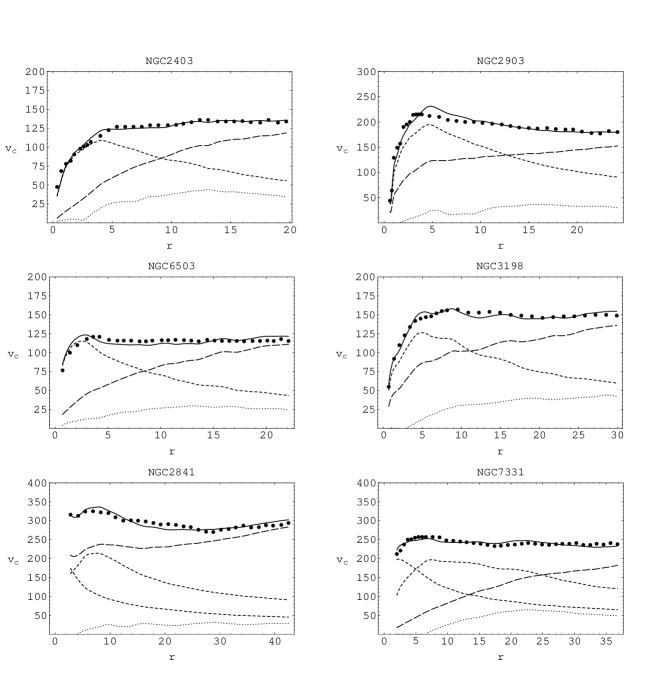
Figure 1: Curves of $v_{C}$ (km/s) vs $r$ (kpc) for the observational data (dots) and the fits from equation (23) (solid). Also shown are the individual contributions from luminous matter (short dashed), the dilaton (long dashed) and gas (dotted). In the case of NGC 2841 and NGC 7331, the lower short dashed curve represents the contribution from the bulge of these galaxies.

For the parameter $M/L$ our results are in very good agreement with previous analyses which employ the dark-halo and the MOND approaches (e.g. Begeman et al. (1991)). The remaining two parameters, $f_{0}$ and $b$, serve only to determine completely the metric, and they do not have a direct physical interpretation other than as part of the scalar field energy density. In Table 2 the best fit parameters are listed, along with the formal $1\sigma$ error in the fitted parameter.

Table 1: Sample of galaxies

Galaxy	Type	Distance	Luminosity	$R_{HI}$
		(Mpc)	($10^{9}M_{\odot}$)	(kpc)
NGC 2403	Sc(s)III	3.25	7.90	19.49
NGC 2903	Sc(s)I-II	6.40	15.30	24.18
NGC 6503	Sc(s)II.8	5.94	4.80	22.22
NGC 3198	Sc(rs)I-I	9.36	9.00	29.92
NGC 2841	Sb	9.46	20.50	42.63
NGC 7331	Sb(rs)I-I	14.90	54.00	36.72

Table 2: Best-fit parameters

Galaxy	(M/L)disk	(M/L)bulge	b	f0
			(kpc)	(kpc-1)
NGC 2403	1.75	–	1.63	0.0116
	0.04	–	0.003	$5.7\times 10^{-4}$
NGC 2903	2.98	–	8.33	0.0043
	0.12	–	0.03	$4.0\times 10^{-4}$
NGC 6503	2.12	–	1.79	0.013
	0.09	–	0.01	$8.7\times 10^{-4}$
NGC 3198	2.69	–	7.83	0.0054
	0.08	–	0.02	$3.0\times 10^{-4}$
NGC 2841	5.39	3.25	13.85	0.0039
	0.34	0.36	0.16	$2.5\times 10^{-4}$
NGC 7331	5.06	1.11	0.845	0.0013
	0.23	0.06	0.002	$8.9\times 10^{-5}$

5 Conclusions.

In this work we have obtained an exact, axially symmetric and static solution to the field equations of gravity coupled with a scalar field. This solution has been successfully employed as a model for a spiral galaxy, and in particular, we have been able to reproduce the RC of matter in these galaxies with an excellent agreement, both with the observations themselves and with previous analyses of this kind of data.

It should be stressed that, although our model has three parameters to be fitted, which in general allows for a great flexibility, they are obtained from a theory that is of a fundamental nature, namely, the low energy limit of a family of unification theories. This makes the calculations herein shown to be natural since no ad hoc hypotheses are needed, in contrast to the dark halo or the MOND models. We conclude that this work enables us to state that scalar fields are strong candidates to constitute the dark matter, not only at a cosmological scale, but also within spiral galaxies.

Appendix A Some geometrical aspects of the metric.

In order to gain some insight into the solution (18), we shall consider a couple of issues related to the geometrical and topological aspects of the metric. By defining:

$$x_{1}=\ln\sqrt{r^{2}+b^{2}\sin^{2}\theta},$$

$$x_{2}=\arctan\left(\frac{\cot\theta}{\sqrt{1+b^{2}/r^{2}}}\right),$$

$$x_{3}=\varphi,$$

$$x_{4}=f_{0}t,$$

we have:

$$ds^{2}=\frac{1}{f_{0}r_{0}}e^{2x_{1}}(dx_{1}^{2}+dx_{2}^{2}+dx_{3}^{2}-c^{2}dx_{4}^{2}).$$ (A1)

From this, it can be argued that our coordinates ($\theta,\varphi$) are not really angles, but in fact just cartesian coordinates. This, however, can only be stated if we know the global topology of our space-time, which we do not. As a counterexample, we can consider the 2-torus, ${\cal T}^{2}$; in this case, the metric is not only conformally flat but in fact flat altogether, i.e., $ds^{2}=dx^{2}+dy^{2}$; with a proper rescaling, this can be written $ds^{2}=d\theta_{1}^{2}+d\theta_{2}^{2}$, where now $\theta_{1}$ and $\theta_{2}$ vary from $0$ to $2\pi$ and can be thought of effectively as angles. A similar example is the 2-sphere, ${\cal S}^{2}$. Therefore, our point of view is that, since interpreting ($r,\theta,\varphi$) as spherical-like coordinates allows us to reproduce the rotation curves for galaxies, we can consider them in such way, and in particular, $\varphi$ does represent angles about the axial direction.

Appendix B Dark-halo profiles and the MOND hypothesis.

The most commonly accepted approach to explain the RC is to assume that there is some kind of unseen matter around the visible part of the galaxy, forming what is usually called a ‘halo’; then, a mass density profile for this dark matter is formulated and combined with data from the visible and 21 cm observations, and the model is fitted to the RC as obtained from red-shifts in the galaxy. A quite broad family of density profiles is given by (Zhao (1996)):

$$\rho_{halo}(r)=\frac{\rho_{c}}{(r/r_{c})^{\gamma}[1+(r/r_{c})^{\alpha}]^{(\beta-\gamma)/\alpha}},$$

where $\rho_{0}$ is the central density and $r_{c}$ is the ‘core’ radius, both of the halo. In particular, the simplest and most widely used profile is the so called modified isothermal sphere (MIS), for which $(\alpha,\beta,\gamma)=(2,2,0)$. This model is attractive because there are cosmological arguments which seem to suggest that, under the suitable conditions, astronomical objects of this kind might actually evolve, the dark matter being cold or hot depending on the evolutionary arguments (see, e.g., Kravtsov et al. (1998) and references therein); however, a completely satisfactory evolution scenario remains to be derived. In the actual fitting procedure, it is usually more convenient to work with the asymptotic circular velocity $v_{h}$ obtained from the isothermal sphere halo, by applying the virial theorem and Newton’s law:

$$v_{h}=\sqrt{4\pi G\rho_{0}r_{c}^{2}}.$$

Beginning with the luminosity observations, $L(r)$, there are three parameters to be adjusted (four in the case of galaxies with separate observations from the disk and the bulge): the ratio $M/L$, usually assumed to be constant over the whole optical disk, the core radius $r_{c}$ and the asymptotic velocity $v_{h}$.

The other approach we shall consider here is known as the modified Newtonian dynamics (MOND), which was proposed by Milgrom (1983); in this case there is no dark matter at all, rather a deviation from the usual Newton’s second law would occur when one is dealing with very ‘small’ accelerations, where ‘small’ means small with respect to some (in principle, universal) critical acceleration parameter, $a_{0}$. Instead of ${\bf F}=m_{g}{\bf a}$, one would write:

$${\bf g}_{N}=\mu(a/a_{0}){\bf a},$$ (B1)

where ${\bf g}_{N}$ is the conventional gravitational acceleration, ${\bf a}$ is the true acceleration of a particle with respect to some fundamental frame ($a\equiv|{\bf{a}|}$), and $\mu$ is a function of $a/a_{0}$ of which only the asymptotic forms $\mu(a/a_{0}\gg 1)\approx 1$, $\mu(a/a_{0}\ll 1)\approx a/a_{0}$ are known. It can then be seen that for accelerations much larger than the acceleration parameter $a_{0}$, $\mu\approx 1$ and we recover the Newtonian dynamics. For the rotation law, the usual expression remains to be valid: $v_{C}^{2}/r=a$, and also $g_{N}\approx MGr^{-2}$; combining this with equation (B1), we get the asymptotic velocity:

$$v_{C}^{4}=GMa_{0}.$$

In this case the acceleration parameter $a_{0}$ can be taken as fixed so there is only one free parameter, again the ratio $M/L$. Alternatively, $a_{0}$ can also be considered as a free parameter. Although this approach works very well when fitting the rotation curves, there is no a priori reason to believe that a deviation of this kind could indeed occur, so this is usually considered to be a purely phenomenological description.

References

- Begeman et al. (1991) Begeman K. G., Broeils A. H. Sanders R. H., 1991, MNRAS, 249, 523
- Cho & Keum (1998) Cho Y. M., Keum Y. Y., 1988, Class. Quantum Grav., 15, 907
- Damour & Esposito-Farèse (1992) Damour T., Esposito-Farèse G., 1992, Class. Quantum Grav., 9, 2093
- Damour & Esposito-Farèse (1993) Damour T., Esposito-Farèse G., 1993, Phys. Rev. Lett., 70, 2220
- Frolov (1999) Frolov A. V., 1999, Class. Quantum Grav., 16, 407
- Guzmán & Matos (1999) Guzmán F. S., Matos T., 1999, in Proceedings of the VIII Marcel Grossman Meeting, ed. D. Ruffini et al. (Singapore: World Scientific), 333
- Guzmán & Matos (2000) Guzmán F. S., Matos T., 2000, Class. Quantum Grav., 17, L9
- Kent (1987) Kent S. M., 1987, AJ, 93, 816
- Kravtsov et al. (1998) Kravtsov A. V., Klypin A. A., Bullock J. S., Primack J. R., 1998, ApJ, 502, 48
- Matos (1989) Matos T., 1989, Ann. Phys. (Leipzig), 46, 462
- Matos (1994) Matos T., 1994, J. Math. Phys., 35, 1302
- Matos (1995) Matos T., 1995, Math. Notes, 58, 1178
- Milgrom (1983) Milgrom M., 1983, ApJ, 270, 371
- Peebles (1999) Peebles P. J .E. 1999, preprint astro-ph/9910350.
- Oort (1932) Oort J., 1932, Bull. Astron. Inst. Neth., 6, 249
- Zhao (1996) Zhao H. S., 1996, MNRAS, 278, 488
- Zwicky (1933) Zwicky F., 1933, Helv. Phys. Acta, 6, 110