Possible explanation for star-crushing effect in binary neutron star simulations

Abstract

A possible explanation is suggested for the controversial star-crushing effect seen in numerical simulations of inspiraling neutron star binaries by Wilson, Mathews and Marronetti (WMM). An apparently incorrect definition of momentum density in the momentum constraint equation used by WMM gives rise to a post-1-Newtonian error in the approximation scheme. We show by means of an analytic, post-1-Newtonian calculation that this error causes an increase of the stars’ central densities which is of the order of several percent when the stars are separated by a few stellar radii, in agreement with what is seen in the simulations.

A controversial issue in the astrophysics community recently has been the claim by Wilson, Mathews and Marronetti (WMM), based on numerical simulations, that inspiraling binary neutron stars are subject to a general-relativistic crushing force that cause them to individually collapse to black holes before they merge [2, 3, 4, 5]. Such a crushing force, if it existed, would have profound implications for current efforts to detect gravitational waves from such systems with LIGO, VIRGO and other ground based detectors. The WMM claim has been disputed by several researchers utilizing a variety of approximate analytical and numerical techniques [6, 7, 8], and recent independent numerical simulations using the same approximation scheme as WMM show no crushing effect [9]. In this paper we suggest an explanation for the star-crushing effect perceived by WMM.

We start with the standard ADM equations. The metric is

$$ds^{2}=-(\alpha^{2}-\beta_{i}\beta^{i})dt^{2}+2\beta_{i}dx^{i}dt+\gamma_{ij}dx^{i}dx^{j},$$ (1)

so that the lapse function is $\alpha$ and the shift vector is $\beta^{i}$. The extrinsic curvature $K_{ij}$ is given by

$$\dot{\gamma}_{ij}=-2\alpha K_{ij}+D_{i}\beta_{j}+D_{j}\beta_{i},$$ (2)

where $D_{i}$ is the derivative operator associated with $\gamma_{ij}$ and dots denote derivatives with respect to $t$. The Hamiltonian constraint is

$${}^{(3)}R-K_{ij}K^{ij}+K^{2}=16\pi\rho_{H},$$ (3)

where ${}^{(3)}R$ is the Ricci scalar of $\gamma_{ij}$, $K\equiv\gamma^{ij}K_{ij}$, $n^{\alpha}$ is the normal to the $t=$ const surface given by $n_{\beta}=-\alpha(dt)_{\beta}$, and $\rho_{H}=T_{\alpha\beta}n^{\alpha}n^{\beta}$. The momentum constraint is

$$D_{i}(K^{ij}-\gamma^{ij}K)=8\pi S^{j},$$ (4)

where $S^{\alpha}\equiv-h^{\alpha\beta}T_{\beta\gamma}n^{\gamma}$ and $h^{\alpha\beta}\equiv g^{\alpha\beta}+n^{\alpha}n^{\beta}$ is the projection tensor. [Here Greek indices run over $(0,1,2,3)$ and Roman indices over $(1,2,3)$.] Finally the trace of the space-space part of Einstein’s equation is

$$4\pi\alpha S = {\dot{K}}+D^{i}D_{i}\alpha-\beta^{l}D_{l}K$$ (6)

$$-{\alpha\over 4}\left[{}^{(3)}R+3K^{ij}K_{ij}+K^{2}\right],$$

where $S\equiv h^{\alpha\beta}T^{\alpha\beta}$.

The main elements of the WMM approximation scheme are as follows [2, 3, 4, 5]: (i) They use the standard perfect fluid equations to evolve the fluid in the background metric (1). The stress-energy tensor is

$$T_{\alpha\beta}=({\bar{\rho}}+p)u_{\alpha}u_{\beta}+pg_{\alpha\beta},$$ (7)

where $u^{\alpha}$ is the 4-velocity, $p$ is the pressure and ${\bar{\rho}}$ is the energy density. The equations of motion are $\nabla_{\alpha}T^{\alpha\beta}=0$ and $\nabla_{\alpha}(nu^{\alpha})=0$, where $n$ is the baryon number density. (ii) They work in a co-rotating coordinate system of the form (1), so that the large $r$ boundary condition on the shift vector is $\beta_{i}(x^{j})=\epsilon_{ijk}\Omega^{j}x^{k}+O(r^{0})$, where $\Omega^{j}$ is the orbital angular velocity. (iii) They impose that the spatial metric $\gamma_{ij}$ be conformally flat, $\gamma_{ij}=\varphi^{4}{\bar{\gamma}}_{ij},$ where ${\bar{\gamma}}_{ij}$ is flat and time independent. By decomposing the extrinsic curvature as $K_{ij}=A_{ij}+K\gamma_{ij}/3$ where $A_{ij}$ is traceless, and combining with (2) and the conformal flatness condition one gets

$$K={-6{\dot{\varphi}}\over\varphi\alpha}+{1\over\alpha}D_{i}\beta^{i}$$ (8)

and

$$A_{ij}={1\over 2\alpha}\left[D_{i}\beta_{j}+D_{j}\beta_{i}-{2\over 3}(D_{k}\beta^{k})\gamma_{ij}\right].$$ (9)

Using the relations (8) and (9), the Hamiltonian constraint (3), the momentum constraint (4) and the dynamical equation (6) can be written schematically as

$${\dot{\varphi}} = F_{1}[\varphi,\beta^{i},\alpha],$$ (10)

$$0 = F_{2}^{i}[\beta^{j},\alpha,\varphi,{\dot{\varphi}}],$$ (11)

$${\ddot{\varphi}} = F_{3}[\varphi,{\dot{\varphi}},\alpha,\beta^{k}],$$ (12)

for some functionals $F_{1}$, $F_{2}^{i}$ and $F_{3}$. (iv) They use a quasi-equilibrium approximation scheme which means that they substitute ${\dot{\varphi}}={\ddot{\varphi}}=0$ into Eqs. (10)–(12). (v) They substitute the maximal slicing condition $K=0$ into the resulting equations. This yields a system of equations in which one can solve for $\alpha$, $\varphi$, and $\beta^{i}$ at each instant from $T_{\alpha\beta}$.

We now turn to a description of the apparent error in the momentum constraint equation used by WMM. Consider the following two inequivalent definitions of momentum density. The first is ${\bar{S}}^{\alpha}\equiv-h^{\alpha\beta}T_{\beta\gamma}n^{\gamma},$ which is just the quantity which appears in the momentum constraint (4). Using the perfect fluid stress energy tensor (7) and the notations $W\equiv-n_{\beta}u^{\beta}=\alpha u^{t}$ and $\sigma\equiv{\bar{\rho}}+p$, it can be written as

$${\bar{S}}^{\alpha}=W\sigma h^{\alpha\beta}u_{\beta}.$$ (13)

The second definition is simply the expression (13) without the projection tensor:

$${\hat{S}}^{\alpha}=W\sigma u^{\alpha}.$$ (14)

WMM appear to confuse the two different quantities (13) and (14). They define only a 3-vector $S_{i}$; this definition [Eq. (47) of Ref. [3]] is compatible with both definitions (13) and (14), since ${\bar{S}}_{i}={\hat{S}}_{i}$ (but ${\bar{S}}_{t}\neq{\hat{S}}_{t}$). However, the 4-vector $S_{\alpha}$ appears in some of their equations. Their hydrodynamic equations are correct only if their $S_{\alpha}$ is interpreted to be ${\hat{S}}_{\alpha}$, while their momentum constraint is correct only if $S_{\alpha}$ is interpreted to be ${\bar{S}}_{\alpha}$.

This confusion apparently gives rise to an error in their equation for the shift vector. WMM solve for the shift vector by combining the relation (9) with the assumption $K=0$ and with the momentum constraint (4). The resulting equation for the shift vector is

$${\bar{D}}^{2}\beta^{i}+{1\over 3}{\bar{D}}^{i}({\bar{D}}_{k}\beta^{k})={\bar{\Lambda}}^{ij}{\bar{D}}_{j}\ln(\alpha/\varphi^{6})+16\pi\alpha\varphi^{4}{\bar{S}}^{j},$$ (15)

where ${\bar{D}}_{i}$ is the derivative operator associated with the flat metric ${\bar{\gamma}}_{ij}$, and ${\bar{\Lambda}}^{ij}\equiv{\bar{D}}^{i}\beta^{j}+{\bar{D}}^{j}\beta^{i}-2({\bar{D}}_{k}\beta^{k}){\bar{\gamma}}^{ij}/3.$ Equation (15) agrees with WMM’s corresponding Eq. (33) of Ref. [3]. However, WMM then rewrite their variable $S^{j}$ in terms of $S_{j}=W\sigma u_{j}$. For the correct variable $S^{j}={\bar{S}}^{j}$, we have ${\bar{S}}^{j}=\varphi^{-4}{\bar{S}}_{j}=\varphi^{-4}W\sigma u_{j}$. For the incorrect variable ${\hat{S}}^{j}$ we have instead

$${\hat{S}}^{j}=W\sigma\left[\varphi^{-4}u_{j}-{W\over\alpha}\beta^{j}\right].$$ (16)

Inserting Eq. (16) into Eq. (15), WMM obtain the equation [Eq. (41) of Ref. [3], also Eq. (15) of Ref. [5]]

$${\bar{D}}^{2}\beta^{j}+ {1\over 3}{\bar{D}}^{j}({\bar{D}}_{k}\beta^{k})={\bar{\Lambda}}^{ij}{\bar{D}}_{i}\ln(\alpha/\varphi^{6})$$ (18)

$$+16\pi\alpha\varphi^{4}W\sigma\left[\varphi^{-4}u_{j}-\epsilon_{0}{W\over\alpha}\beta^{j}\right],$$

with $\epsilon_{0}\equiv 1$ [10]. The correct version of this equation is given by $\epsilon_{0}=0$; see, for example, Eq. (2.16) of Ref. [7].

We now turn to calculating the leading order effect of this error on the stars’ central densities. We define a fictitious stress-energy tensor $\Delta T_{\alpha\beta}$ by $G_{\alpha\beta}[g_{\mu\nu}]=8\pi\left[{}^{(F)}T_{\alpha\beta}+\Delta T_{\alpha\beta}\right],$ where $g_{\mu\nu}$ is the metric obtained by solving the WMM equations and ${}^{(F)}T_{\alpha\beta}$ is the fluid stress-energy tensor (7). It is a useful point of view to regard Einstein’s equation as being satisfied exactly, but with an extra type of matter present whose (conserved) stress tensor is $\Delta T_{\alpha\beta}$ and which interacts with the neutron stars only gravitationally. The fictitious stress-energy tensor is of post-1-Newtonian order, although without the error term in Eq. (18) it would have been of post-2-Newtonian order. Our approach will be to calculate $\Delta T_{\alpha\beta}$ analytically to post-1-Newtonian order, and then, starting from a correct, post-1-Newtonian description of the binary, to solve for the perturbation to the stellar structure that is linear in $\Delta T_{\alpha\beta}$.

In our calculations, it will be sufficient to restrict attention to stationary solutions for which the vector field $\partial/\partial t$ is a killing vector field, since the numerical, dynamic solutions to the WMM equations relax to such stationary states [3]. There are two contributions to $\Delta T_{\alpha\beta}$: (i) a direct contribution due to the error term in Eq. (18), and (ii) an indirect contribution due to the fact that the first error causes a non-zero $K$ and invalidates the maximal slicing assumption.

We first calculate the direct contribution. We can decompose the fictitious stress energy tensor as

$$\Delta T^{\alpha\beta}=\Delta\rho\,n^{\alpha}n^{\beta}+2n^{(\alpha}\Delta S^{\beta)}+\Delta S^{\alpha\beta}_{({\rm TF})}+{1\over 3}h^{\alpha\beta}\Delta S,$$ (19)

where $\Delta\rho\equiv\Delta T_{\alpha\beta}n^{\alpha}n^{\beta}$, $\Delta S^{\alpha}\equiv-(g^{\alpha\beta}+n^{\alpha}n^{\beta})\Delta T_{\beta\gamma}n^{\gamma}$, $\Delta S\equiv(g^{\alpha\beta}+n^{\alpha}n^{\beta})\Delta T_{\alpha\beta}$ and $\Delta S^{\alpha\beta}_{(TF)}$ is orthogonal to $n^{\alpha}$ and tracefree. We define $\Delta\beta^{i}\equiv\beta^{i}-{\bar{\epsilon}}^{ijk}\Omega_{j}x_{k}$, where ${\bar{\epsilon}}^{ijk}$ is the volume element associated with the flat metric ${\bar{\gamma}}_{ij}$ and $x^{i}$ are Cartesian coordinates associated with ${\bar{\gamma}}_{ij}$; thus $\Delta\beta^{i}\to 0$ as $r\to\infty$. Rewriting Eq. (18) in terms of $\Delta\beta^{i}$ and the contravariant components of the 4-velocity and taking the post-1-Newtonian limit yields

$${\bar{D}}^{2}\Delta\beta^{j}+ {1\over 3}{\bar{D}}^{j}({\bar{D}}_{k}\Delta\beta^{k})=$$ (21)

$$16\pi\rho_{M}\left[v^{j}+(1-\epsilon_{0})({\bf\Omega}\times{\bf x})^{j}\right],$$

where $\rho_{M}$ is the Newtonian mass density and $v^{i}=dx^{i}/dt$ is the 3-velocity in the rotating frame (1). From Eq. (21) we see that there is there is a direct contribution

$$-\epsilon_{0}({\bf\Omega}\times{\bf x})\rho_{M}$$ (22)

to the quantity $\Delta S^{i}$.

Consider now the indirect contribution. Using Eq. (8) and the stationarity condition ${\dot{\varphi}}=0$ yields

$$K={1\over\alpha}\left[{\bar{D}}_{i}\beta^{i}+6\beta^{i}{\bar{D}}_{i}\ln\varphi\right].$$ (23)

We now solve Eq. (21) for the quantity ${\bar{D}}_{i}\beta^{i}={\bar{D}}_{i}\Delta\beta^{i}$, insert the result into Eq. (23), make use of the Newtonian continuity equation in the rotating frame ${\bar{D}}_{i}(\rho_{M}v^{i})=-{\dot{\rho}_{M}}=0$, and use the post-1-Newtonian relation $\varphi=1-\Phi/2$ between the conformal factor $\varphi$ and the Newtonian potential $\Phi$. The result is

$$K=-3\epsilon_{0}({\bf\Omega}\times{\bf x})\cdot{\bf\nabla}\Phi.$$ (24)

Now WMM insert the assumption $K=0$ into Eqs. (3), (4) and (6). Since $K$ is actually non-vanishing, this gives rise to the following contributions to $\Delta T_{\alpha\beta}$: $\Delta\rho=K^{2}/24\pi$, $\Delta S^{i}=-D^{i}K/12\pi$, and $\Delta S=({\dot{K}}-\beta^{i}D_{i}K-\alpha K^{2}/2)/4\pi\alpha$. Using the relation (24), taking the post-1-Newtonian limit, adding the direct contribution (22), using the stationarity assumption and letting $\epsilon_{0}\to 1$ finally yields [11] $\Delta\rho=0$,

$$\Delta{\bf S} = {1\over 4\pi}{\bf\nabla}\cdot\left[({\bf\Omega}\times{\bf x})\cdot{\bf\nabla}\Phi\right]-({\bf\Omega}\times{\bf x})\rho_{M},$$ (25)

$$\Delta S = {3\over 4\pi}\left[\left({\bf\Omega}\times{\bf x}\right)\cdot{\bf\nabla}\right]^{2}\Phi.$$ (26)

We next calculate the effect of the fictitious stress energy tensor (25)–(26) on the neutron stars’ central densities. Focus attention on one of the two stars, say star A. We define the two dimensionless parameters $\epsilon\equiv M/R$ and $\kappa\equiv R/L$, where $M$ is the mass and $R$ the radius of either star, and $L$ is the orbital separation. We will work to the leading non-vanishing order in $\kappa$, which will turn out to be linear in $\kappa$. Now it is known that the leading order (tidal) fractional corrections to the internal structure of star A due to the other star scale as $\kappa^{3}$, to post-1-Newtonian order as well as in Newtonian gravity [8]; we can neglect these corrections. Hence, accurate to $O(\kappa^{2})$, we can find a non-rotating coordinate system $({\bar{t}},{\bar{x}}^{i})$ near star A in which the metric is that of an isolated neutron star. These coordinates are related to the original co-rotating coordinates $(t,x^{i})$ of the line element (1) by

$$t = {\bar{t}}+{\dot{z}}^{i}({\bar{t}}){\bar{x}}^{i}$$ (27)

$$R_{ij}(t)x^{j} = z^{i}({\bar{t}})+{\bar{x}}^{i}.$$ (28)

Here $R_{ij}(t)$ is the rotation matrix satisfying ${\dot{R}}_{il}(t)=\epsilon_{ijk}\Omega_{j}R_{kl}(t)$, $z^{i}(t)\equiv R_{ij}(t)z^{j}_{A}$, and $z^{j}_{A}$ is the (time-independent) coordinate location of the center of star A in the $(t,x^{i})$ coordinates. The transformation (27)–(28) is approximate but is sufficiently accurate for our calculation.

Next, we combine Eqs. (19) and (25)–(26) together with $n^{\mu}=(1,-\beta^{i})/\alpha\approx(1,-{\bf\Omega}\times{\bf x})$ to obtain the contravariant components of $\Delta T^{\alpha\beta}$ in the $(t,x^{i})$ coordinate system. We then use the zeroth order metric $ds^{2}=-dt^{2}+2({\bf\Omega}\times{\bf x})_{i}\,dt\,dx^{i}+d{\bf x}^{2}$ to obtain the covariant components $\Delta T_{\alpha\beta}$, and finally use the transformation (27)–(28) to calculate the components $\Delta T_{{\bar{\alpha}}{\bar{\beta}}}$ in the $({\bar{t}},{\bar{x}}^{i})$ coordinates, discarding all post-2-Newtonian terms. The result is $\Delta T_{{\bar{t}}{\bar{t}}}=\Delta\rho_{F}$, $\Delta T_{{\bar{t}}{\bar{i}}}=-\Delta S^{i}$ and $\Delta T_{{\bar{i}}{\bar{j}}}=\Delta p_{F}\delta_{{\bar{i}}{\bar{j}}}+Q_{{\bar{i}}{\bar{j}}}$, where $\Delta S^{i}$ is given by Eq. (25),

$$\Delta\rho_{F}=-{1\over 2\pi}\left[\left({\bf\Omega}\times{\bf x}\right)\cdot{\bf\nabla}\right]^{2}\Phi+2({\bf\Omega}\times{\bf x})^{2}\rho_{M}$$ (29)

is the fictitious density,

$$\Delta p_{F}={1\over 12\pi}\left[\left({\bf\Omega}\times{\bf x}\right)\cdot{\bf\nabla}\right]^{2}\Phi+{2\over 3}({\bf\Omega}\times{\bf x})^{2}\rho_{M}$$ (30)

is the fictitious pressure, and where $Q_{{\bar{i}}{\bar{j}}}$ is a traceless tensor that does not contribute to the leading order change in central density. In deriving Eqs. (29)–(30) [but not in deriving the expression (25) for $\Delta T_{{\bar{t}}{\bar{i}}}$] we replaced ${\bf\Omega}\times{\bf z}_{A}$ by ${\bf\Omega}\times{\bf x}$, which is valid to leading order in $\kappa$.

Consider now the case where star A is non-rotating and hence spherically symmetric. Then, the fictitious momentum density $\Delta T_{{\bar{t}}{\bar{i}}}$ will not affect the central density of the star [12], so we can restrict attention to $\Delta\rho_{F}$ and $\Delta p_{F}$. To leading order in $\kappa$, we can replace $\Phi$ and $\rho_{M}$ in Eqs. (29)–(30) by the self potential $\Phi_{A}$ and the mass density $\rho_{M,A}$ of star A, and we can replace the quantity ${\bf\Omega}\times{\bf x}$ by ${\bf\Omega}\times{\bf z}_{A}$. The first term in Eqs. (29) is then proportional to $\partial^{2}\Phi_{A}/\partial y^{2}$ with a suitable choice of $y$-axis, which becomes ${\bf\nabla}^{2}\Phi_{A}/3=4\pi\rho_{M,A}/3$ when we average over solid angles about the center of star A. Hence to leading order in $\kappa$ we obtain

$$\Delta\rho_{F} = {4\over 3}\ v_{\rm orb}^{2}\ \rho_{M,A},\ \ \ \ \Delta p_{F}={7\over 9}\ v_{\rm orb}^{2}\ \rho_{M,A},$$ (31)

where ${\bf v}_{\rm orb}={\bf\Omega}\times{\bf z}_{A}$ is the orbital velocity.

It is clear that the fictitious density and pressure (31) will cause a fractional increase in the central density of star A proportional to $\epsilon\,\kappa$ at leading order. To evaluate the constant of proportionality we solve for the perturbation to the structure of star A using the following modified form of the TOV equations [13]:

$${dm\over dr} = 4\pi r^{2}\left[\rho+\Delta\rho_{F}\right],$$ (32)

$${dp\over dr} = -{(\rho+p)\left[m+4\pi r^{3}(p+\Delta p_{F})\right]\over r(r-2m)}.$$ (33)

Our procedure consists of: (i) solving Eqs. (32)–(33) without the correction terms to obtain the unperturbed structure of the star. We use the same stellar model as used in Ref. [5], described by the polytropic equation of state $p=K\rho_{M}^{\Gamma}$, $\rho=\rho_{M}+K\rho_{M}^{\Gamma}/(\Gamma-1)$, where $\rho_{M}$ is the rest-mass density, $\Gamma=2$, and $K=1.8\times 10^{5}$ erg cm³ gr^-2. We choose a central density for the unperturbed star of $\rho_{c}=5.93\times 10^{14}$ gr cm^-3, which implies a baryonic mass of $1.62M_{\odot}$ and a total mass of $1.51M_{\odot}$. (ii) We use Eqs. (31) to calculate $\Delta\rho_{F}$ and $\Delta p_{F}$. (iii) We insert these $\Delta\rho_{F}$ and $\Delta p_{F}$ into into Eqs. (32)–(33), and adjust the choice of central density $\rho_{c}$ until a perturbed stellar model with the same total baryonic mass of $1.62M_{\odot}$ is obtained. The result is shown in Fig. 1, where we choose the stellar separation to be given by $\kappa=R/L=1/4$, corresponding to $v_{\rm orb}=0.132$. The central density has increased by $\sim 15\%$.

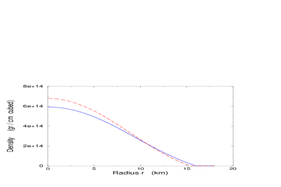
FIG. 1.: Consider a neutron star described by a polytropic $\Gamma=2$ equation of state, at an orbital separation of 4 stellar radii from another similar neutron star. The density profile of such a star will be very close to that of an isolated star, which is shown as the solid line. When the leading order effects of the erroneous term in the momentum constraint equation are included, the result is the dashed line.

Turn next to the case when star A is rigidly co-rotating. The fractional corrections to its internal structure due to its own rotation scale as $\kappa^{3}$, and therefore to leading order in $\kappa$ the above analysis of the effects of $\Delta p_{F}$ and $\Delta\rho_{F}$ is still valid. However, there is now in addition a gravitomagnetic interaction between the fluid’s velocity and the fictitious momentum density $\Delta T_{{\bar{t}}{\bar{i}}}$. A straightforward computation shows that the radial component of the gravitomagnetic force averaged over solid angles is

$$-{8\over 3}\rho_{M}\Omega^{2}r\left[2\lambda(r)+r\Phi^{\prime}(r)\right],$$ (34)

where $\lambda(r)$ is given by $(r\partial_{r}+3)\lambda=\Phi$ with $\lambda$ finite as $r\to 0$. This force gives rise to a fractional change in central density proportional to $\epsilon\,\kappa^{2}$. Evaluating this change numerically at $\kappa=1/4$ for the same stellar model as above gives a contribution to $\delta\rho_{c}/\rho_{c}$ of less than one percent. Therefore, the dominant contribution to $\delta\rho_{c}$ should be that from $\Delta\rho_{F}$ and $\Delta p_{F}$, and the crushing effect should be seen in the co-rotating case as well as in the non-rotating case.

To conclude, we compare our predictions with the behavior seen in the WMM simulations: (i) The predicted magnitude of $\delta\rho_{c}/\rho_{c}$ agrees with that seen. (ii) The scaling $\delta\rho_{c}\propto\kappa\propto 1/L$ is not inconsistent with the scaling seen in the simulations [14]. (iii) Our analysis cannot explain the claim by WMM [4] that the crushing effect is not seen in the co-rotating case. In any case, it should be straightforward to verify or falsify our proposed explanation by re-running the simulations without the extra term in the momentum constraint equation.

I thank Greg Cook, Grant Mathews, Saul Teukolsky and Ira Wasserman for helpful discussions. This research was supported in part by NSF grant PHY–9722189 and by a Sloan Foundation fellowship.

REFERENCES

[1] Also Center for Radiophysics and Space Research,
Cornell University, Ithaca, NY 14853.
[2]
J. R. Wilson and G. J. Mathews, Phys. Rev. Lett. 75,
4161 (1995); P. Marronetti, G.J. Mathews, J.R. Wilson, Phys. Rev. D
58, 042822 (1998).
[3]
J. R. Wilson, G. J. Mathews and P. Marronetti, Phys. Rev. D. 54,
1317 (1996).
[4]
G.J. Mathews and J.R. Wilson, Ap. J. 482, 929
(1997).
[5]
G. J. Mathews, P. Marronetti, J. R. Wilson,
Phys. Rev. D 58, 043003 (1998).
[6]
D. Lai, Phys. Rev. Lett. 76, 4878 (1996);
A. G. Wiseman, Phys. Rev. Lett. 79, 1189
(1997); P. R. Brady and S. A. Hughes, Phys. Rev. Lett. 79, 1186 (1997);
T. W. Baumgarte, G. B. Cook, M. A. Scheel, S. L. Shapiro, and S. A. Teukolsky, Phys. Rev. Lett. 79, 1182
(1997); also Phys. Rev. D 57 6181 (1998) and
Phys. Rev. D 57, 7299 (1998);
M. Shibata, Prog. Theor. Phys. 96, 317
(1996); Phys. Rev. D 55, 6019 (1997);
K. Taniguchi and M. Shibata,
Phys. Rev. D 56, 798 (1997), ibid, 56, 811 (1997);
M. Shibata, K. Oohara, and
T. Nakamura, Prog. Theor. Phys. 98, 1081 (1997); M. Shibata,
K. Taniguchi, and T. Nakamura, Prog. Theor. Phys. Suppl. 128
295 (1997).
[7]
M. Shibata, T. W. Baumgarte, S. L. Shapiro, Phys. Rev. D 58, 023002 (1998).
[8] K. S. Thorne, Phys. Rev. D, to appear ; E. E. Flanagan, Phys. Rev. D, to appear.
[9]
S. Bonazzola, E. Gourgoulhon and J. Marck,
gr-qc/9810072.
[10]
Equations (41) of Ref. [3] and (15) of Ref. [5] actually differ from Eq. (18) by factors of
and in the first and second terms in the
square brackets. These factors are possibly typos; in any case their
presence or absence changes the system of equations only at
post-2-Newtonian order and hence is irrelevant for the discussion of
this paper.
[11]
There is in addition a post-1-Newtonian contribution to the quantity
which we ignore, since it can be shown
that this contribution does not affect the stars’ central densities
at leading order.
[12] The gravitomagnetic interaction vanishes since the
fluid velocity is zero. There is a force term proportional to the
time derivative of the transverse part of the perturbation to
, but one can show that the radial component of
this force has no spherically symmetric component.
[13]
It would be more consistent to use the post-1-Newtonian version of the
TOV equations rather than the fully relativistic version, but the
results are insensitive to which version we pick.
[14]
Although Ref. [5] suggests that , Fig. 2 of Ref. [5] is not incompatible with a fit of
the form with the two terms comparable at . This paper calculates only the leading order term .