[

Direct Signature of Evolving Gravitational Potential from Cosmic Microwave Background

Abstract

We show that time dependent gravitational potential can be directly detected from the cosmic microwave background (CMB) anisotropies. The signature can be measured by cross-correlating the CMB with the projected density field reconstructed from the weak lensing distortions of the CMB itself. The cross-correlation gives a signal whenever there is a time dependent gravitational potential. This method traces dark matter directly and has a well defined redshift distribution of the window projecting over the density perturbations, thereby avoiding the problems plaguing other proposed cross-correlations. We show that both MAP and Planck will be able to probe this effect for observationally relevant curvature and cosmological constant models, which will provide additional constraints on the cosmological parameters.

]

It is widely accepted that cosmic microwave background (CMB) anisotropies offer a unique environment to study cosmological models. The anisotropies were generated predominantly during recombination at redshift $z\sim 1100$, when the universe was still in a linear regime and the physics at eV energy scale was simple. This allows one to make robust predictions for various cosmological models, which can be compared to an increasing number of observations. However, some degeneracies between cosmological parameters remain even for future satellite missions and these are being further expanded as new parameters are being introduced. The degeneracies are particularly severe between various components affecting the expansion of the universe, such as curvature, cosmological constant or any other term with a more general equation of state [4]. Other cosmological tests must therefore be used to break these degeneracies.

It has been pointed out that in a universe where matter density does not equal critical density the gravitational potential is changing with time, which produces a significant component to the CMB on large scales [5]. This effect is generated at late times and since the gravitational potential is related to the density field through the Poisson’s equation, the effect can also be looked for by cross-correlating CMB with another tracer of density field [6]. Unfortunately, no clean density map out to high redshift exists on large scales. The X-ray background has been suggested as a possible tracer of large scale structure out to $z\sim 3-4$, but the uncertainties associated with the redshift distribution of the sources, relation between X-ray light and underlying mass and the Poisson fluctuations from the nearby sources make this test inconclusive [7, 8].

Recently we developed a method to reconstruct the projected density field out to recombination directly from the CMB anisotropies [9]. The method is based on the gravitational lensing effect, which distorts the pattern of CMB anisotropies [10]. Although the signal to noise for individual structures from such a reconstruction is small, averaging over independent patches of CMB reduces the noise and extracts the signal in a statistical sense. We were able to show that this allows one to extract the power spectrum of density perturbations with high accuracy over two decades in angular scale [11].

In the present paper we use the reconstructed projected density field to cross-correlate it with the CMB itself. If there is a component to the CMB from the time evolving gravitational potential then it should correlate with the projected density field. Most of the signature comes from large angular scales, so we first generalize the method developed in [9] to all sky. Because the small scale CMB anisotropies were generated uniquely during recombination, the weighting of density perturbations as a function of redshift in the projection is well defined. Moreover, gravitational lensing effect depends on the dark matter distribution in the universe, so no assumption of how light traces mass is necessary. This avoids the shortcomings of cross-correlations with X-ray and other tracers of large scale structure mentioned in [6]. In addition, the projected density field is sensitive to matter distribution out to a very high redshift and allows one to test the models where the time dependent potential is generating anisotropies at higher redshifts, such as the curvature dominated models [8, 12]. Here we compute the expected signal to noise of future CMB missions for cosmological constant and curvature dominated models, using both MAP and Planck satellite characteristics. Although we limit to these two families of models we note that other models, such as those with more general equation of state, would also produce a signature that one could look for.

To reconstruct the projected density field we consider the symmetric tensor of products of temperature derivatives transverse to direction $\hat{n}$ [9]

$${\cal H}_{ab}={1\over\sigma_{\cal S}}T_{:a}T_{:b}$$ (1)

where $T_{:a}$, $T_{:b}$ are covariant derivatives of $T$ with respect to the coordinate basis in the tangent space of direction $\hat{n}$, here defined with polar coordinates $(\theta,\phi)$ and $g_{ab}$ is the metric on the sphere. We defined $\sigma_{\cal S}$ so that in the absence of lensing the average over CMB $\langle{\cal H}_{ab}\rangle_{CMB}={1\over 2}g_{ab}$. The tensor can be decomposed into the trace and traceless component as ${\cal H}_{ab}={1\over 2}(1-{\cal S})g_{ab}-{\tilde{{\cal H}}_{ab}}$. From the traceless tensor ${\tilde{{\cal H}}_{ab}}$ one may define two rotationally invariant quantities

$${\cal E}={1\over 2}\nabla^{-2}{\tilde{{\cal H}}_{ab}}^{:a:b}\;\;\,\,\,{\cal B}={1\over 2}\nabla^{-2}{\tilde{{\cal H}}_{ab}}^{:a:c}\epsilon^{a}_{c},$$ (2)

where $\epsilon^{a}_{c}$ is the completely antisymmetric (Levi-Civitta) tensor and $\nabla^{-2}$ is the inverse Laplacian on the sphere.

In the presence of lensing the average of ${\cal H}_{ab}$ becomes [9]

$$\langle{\cal H}_{ab}\rangle_{CMB}=\left({1\over 2}-\kappa\right)g_{ab}-\gamma_{ab}$$ (3)

where $\kappa$ and $\gamma_{ab}$ are the convergence and the shear components of the symmetric shear tensor $\Phi_{ab}$, defined as the covariant derivative of the displacement field on the sphere [15], which encodes the information on the gravitational lensing effect. All rotationally invariant quantities can be decomposed on a sphere into spherical harmonics, $X(\hat{n})=\sum_{lm}a_{X,lm}Y_{lm}(\hat{n})$, where $X$ stands for $T$, $\kappa$, $\cal S$, $\cal E$ or $\cal B$. From equation [3] we find $\langle a_{{\cal S},lm}\rangle=M_{{\cal S}l}a_{\kappa,lm}$, with $M_{{\cal S}l}=2$. The multipole moments of the scalar field $\cal E$ average to $\langle a_{{\cal E},lm}\rangle=M_{{\cal E}l}a_{\kappa,lm}$, where $M_{{\cal E}l}=2(l+2)(l-1)/l(l+1)$ [15], while the average of the pseudo scalar field $\cal B$ identically vanishes in the large scale limit, $\langle a_{{\cal B},lm}\rangle=0$, because gravitational potential from which shear is generated is invariant under the parity transformation. Convergence $\kappa$ can thus be reconstructed in two independent ways from $\cal S$ and $\cal E$, while the third quantity $\cal B$ serves as a check for possible systematics. Note that since convergence is expressed as a quadratic quantity of $T$ its cross-correlation with $T$ gives a non-vanishing 3rd moment. This means it can also be looked for using bispectrum, which is a method independently proposed by [13].

Convergence can be written as a projection of gravitational potential [14, 17] $\kappa=\int_{0}^{\chi_{0}}g(\chi,\chi_{0})\nabla^{2}\phi(\chi)d\chi$. Here $\chi_{0}$ is the comoving radial coordinate at recombination and $g$ is the radial window, defined as $g(\chi,\chi_{0})={r(\chi)r(\chi_{0}-\chi)\over r(\chi_{0})}$. It is a bell shaped curve symmetric around $\chi/2$ and vanishing at 0 and $\chi_{0}$. Here $r(\chi)$ is the comoving angular diameter distance, defined as $K^{-1/2}\sin K^{1/2}\chi$, $\chi$, $(-K)^{-1/2}\sinh(-K)^{1/2}\chi$ for $K>0$, $K=0$, $K<0$, respectively, where $K$ is the curvature. Curvature can be expressed using the present density parameter $\Omega_{0}$ and the present Hubble parameter $H_{0}$ as $K=(\Omega_{0}-1)H_{0}^{2}$. In general $\Omega_{0}$ consists both of matter contribution $\Omega_{m}$ and cosmological constant term $\Omega_{\Lambda}$.

The angular power spectra are defined as $C^{XX^{\prime}}_{l}={1\over 2l+1}\sum_{m}a_{X,lm}^{*}a_{X^{\prime},lm}$. Their ensemble averages are given by [16]

$$C^{XX^{\prime}}_{l}=(4\pi)^{2} \int \beta^{2}d\beta P(\beta)\Delta_{Xl}(\beta,\tau_{0})\Delta_{X^{\prime}l}(\beta,\tau_{0})$$ (4)

$$\Delta_{Xl}(\beta,\tau_{0})= \int_{0}^{\tau_{0}} d\tau\Phi_{\beta}^{l}(\tau_{0}-\tau)S_{X}(\beta,\tau),$$ (5)

where $\Phi_{\beta}^{l}(x)$ are the ultra-spherical Bessel functions and $P(\beta)$ is the primordial power spectrum. Equation 5 only applies to flat and open universes, whereas for the closed universe the eigenvalues of the Laplacian are discrete so the integral over $\beta$ is replaced with a sum over $K^{-{1\over 2}}\beta=3,4,5...$. The source for temperature anisotropies $S_{T}$ is a combination of several terms. These can be decomposed into terms generated during recombination, which consist of Sachs-Wolfe term, Doppler term, intrinsic anisotropy term and anisotropic stress term, and late time term generated by the time dependent gravitational potential (so-called integrated Sachs-Wolfe term or ISW). The latter is only important for low multipole moments. The full form of $S_{T}$ can be found in [16]. The source for convergence is $S_{\kappa}=g\beta^{2}\phi$. It is also useful to define the correlation coefficient ${\rm Corr}^{T\kappa}_{l}=C^{T\kappa}_{l}/(C^{TT}_{l}C^{\kappa\kappa}_{l})^{1/2}$, which is the relevant quantity for the estimation of signal to noise.

Using the above expressions one can compute $C^{TT}_{l}$, $C^{\kappa\kappa}_{l}$ and $C^{T\kappa}_{l}$ for any cosmological model. We performed numerical calculations using a modified version of CMBFAST code [18]. We have verified that $C^{\kappa\kappa}_{l}$ agrees with previous calculations which were done in the small scale limit [17], as well as with the alternative all-sky expressions given in [15]. The results for $({\rm Corr}^{T\kappa}_{l})^{2}$ are shown in figure 1 for a representative set of models. The correlation coefficient in a cosmological constant model is substantial only for very low $l$ and rapidly drops on smaller scales. In a curvature dominated model with the same $\Omega_{m}$ the correlation coefficient is larger to start with and also drops less rapidly with $l$. This indicates that one will be able to set stronger limits on curvature than on cosmological constant, which is confirmed below with a more detailed analysis. The reason is that in a cosmological constant model the gravitational potential changes only at late times ($z\raise 2.9pt\hbox{$\scriptstyle<$}\lower 0.5pt\hbox{$\scriptscriptstyle\sim$}\;1$ for reasonable values of $\Omega_{m}$), while in a curvature dominated model potential changes also at higher redshift. This leads to two effects. First is that in a cosmological constant model ISW is comparable to other terms only for the lowest multipoles, while in a curvature model ISW dominates up to higher $l$ [12]. Second is that the window $g$ peaks at relatively high redshift $z\sim 3$ and so is able to pick up correlations with ISW from open universe better than that from cosmological constant universe. We have also calculated the correlation coefficient for a flat model. It is small for all $l$, $({\rm Corr}^{T\kappa}_{l})^{2}<10^{-3}$, demonstrating that correlations with fluctuations generated at recombination are negligible and the cross-correlation is sensitive to the time dependent gravitational potential only.

FIG. 1.: Square of correlation coefficient $({\rm Corr}^{T\kappa}_{l})^{2}$ as a function of $l$ is shown for open $\Omega_{m}=0.2$ and $\Omega_{m}=0.4$ models (upper and lower dashed curve) and for cosmological constant $\Omega_{m}=0.2$ and $\Omega_{m}=0.4$ models (upper and lower solid curves).

We now address the question of signal detectability with the future CMB missions. We continue to work in multipole moment space and assume we have all sky expansion, which allows us to decouple between different $m$ and $l$ multipole moments. The generalization to incomplete sky coverage can be approximated by inserting appropriate factors of sky coverage fraction $f_{sky}$ in the final expressions. Given two random fields $T$ and $\cal W$ (where $\cal W$ stands for $\cal S$ or $\cal E$) we want to develop a test that maximizes the signal in the presence of correlations against the null hypothesis that there are no correlations. The term that quantifies the correlations is the product between the two fields $X^{\cal W}_{lm}=T_{lm}^{*}{\cal W}_{lm}$ (here and below average with the complex conjugate $(T_{lm}^{*}{\cal W}_{lm}+T_{lm}{\cal W}_{lm}^{*})/2$ is implied). Its expectation value under the null hypothesis of pure noise is $\langle X^{\cal W}_{lm}\rangle_{0}=0$, because the function entering this expression is a three-point function of $T$, which vanishes both for intrinsic fluctuations and for detector noise under the Gaussian assumption. The alternative hypothesis is that of signal which gives $\langle X^{\cal W}_{lm}\rangle_{1}=\langle T_{lm}^{*}{\cal W}_{lm}\rangle=M_{{\cal W}l}C^{T\kappa}_{l}$. The variance under the null hypothesis is

$$\langle X^{\cal W}_{lm}X^{\cal W^{\prime}}_{lm}\rangle_{0}-\langle X^{\cal W}_{lm}\rangle_{0}\langle X^{\cal W^{\prime}}_{lm}\rangle_{0}=$$ (6)

$$( C^{TT}_{l}+N^{TT}_{l})(M_{{\cal W}l}M_{{\cal W^{\prime}}l}C^{\kappa\kappa}_{l}+N^{\cal WW^{\prime}}_{l}),$$ (7)

where $N^{TT}_{l}$ and $N^{\cal WW^{\prime}}_{l}$ are the noise power spectra for CMB anisotropies, $\cal S$, $\cal E$ or their cross-term, respectively.

Both $\cal S$ and $\cal E$ contribute information. If they are uncorrelated then the information contents can be added independently, otherwise the covariance matrix ${\rm Cov}(X^{\cal W}_{lm}X^{\cal W^{\prime}}_{lm})$ has to be diagonalized first. The CMB term $C^{TT}_{l}+N^{TT}_{l}$ is the same for all matrix elements and can be computed using MAP and Planck noise characteristics. For these CMB missions detector noise on large scales will be negligible, hence $N^{TT}_{l}\ll C^{TT}_{l}$. The dominant source of noise in $\cal S$ or $\cal E$ on large scales are the CMB anisotropies. The noise terms involve integrals over the CMB power spectrum and can be computed numerically using the expressions given in [9]. The results are shown in figure 2 both for MAP and Planck. They show that on large scales the CMB noise power spectrum has approximately white noise shape, $N^{\cal W\cal W}_{l}\sim\rm{const}$. At low $l$ $N^{\cal E\cal E}_{l}\sim N^{\cal S\cal S}_{l}/2\gg N^{\cal E\cal S}_{l},C^{\kappa\kappa}_{l}$. Therefore, noise dominates over the signal and the latter can only be extracted in a statistical sense by averaging over multipole moments. Because the off-diagonal term $\langle{\cal E}_{lm}^{*}{\cal S}_{lm}\rangle_{0}$ is much smaller than the two diagonal terms the covariance matrix is nearly diagonal and the information from $\cal S$ and $\cal E$ can be added independently, with $\cal E$ contributing twice the amount of information than $\cal S$. Note also that Planck has a factor of 5 better sensitivity than MAP.

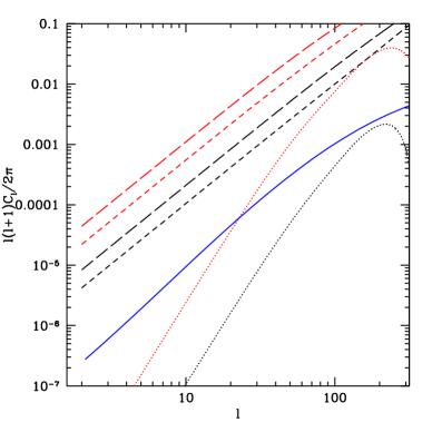
FIG. 2.: Power spectra for noise $N^{\cal S\cal S}_{l}$ (long dashed), $N^{\cal E\cal E}_{l}$ (short dashed), $N^{\cal E\cal S}_{l}$ (dotted) both for Planck (lower curves) and MAP (upper curves) for cosmological constant model with $\Omega_{m}=0.3$. Also shown is power spectrum of convergence $4C^{\kappa\kappa}_{l}$ (solid) for the same model, normalized to $\sigma_{8}=1$.

We now want to combine the signal to noise from different multipole moments to maximize the overall signal to noise. To do this we add up the products weighted with some yet to be determined weights $\alpha_{l}$, $X=\sum_{m,l}\alpha_{l}X_{lm}$. Since the moments are uncorrelated the expectation value and variance are

$$\langle X\rangle_{1} = \sum_{l}(2l+1)\alpha_{l}M_{{\cal W},l}C^{T\kappa}_{l}$$ (8)

$$\langle X^{2}\rangle_{0} = \sum_{l}(2l+1)\alpha_{l}^{2}(C^{TT}_{l}+N^{TT}_{l})(M_{{\cal W}l}^{2}C^{\kappa\kappa}_{l}+N^{\cal WW}_{l}),$$ (9)

while the null hypothesis mean remains $\langle X\rangle_{0}=0$. We want to maximize $S/N=(\langle X\rangle_{1}-\langle X\rangle_{0})/(\langle X^{2}\rangle_{0})^{1/2}$ with respect to $\alpha_{l}$. Taking derivatives with respect to $\alpha_{l}$ and setting the expression to 0 we find $\alpha_{l}=C^{T\kappa}_{l}/(C^{TT}_{l}+N^{TT}_{l})(M_{{\cal W}l}^{2}C^{\kappa\kappa}_{l}+N^{\cal W\cal W}_{l})$. The overall signal to noise is, combining the information from $\cal S$ and $\cal E$

$${S\over N}=\left[f_{sky}\sum_{l}\sum_{\cal W=\cal E,\cal S}{(2l+1)({\rm Corr}^{T\kappa}_{l})^{2}\over(1+{N^{TT}_{l}\over C^{TT}_{l}})(1+{N^{\cal W\cal W}_{l}\over M_{{\cal W}l}^{2}C^{\kappa\kappa}_{l}})}\right]^{1/2},$$ (10)

where we inserted $f_{sky}$ to account for the fact that the number of multipoles will be smaller if only some fraction of the sky will be measured. We have expressed the signal in terms of number of standard deviations above the noise. To express it in terms of confidence limits a more detailed analysis with Monte Carlo simulations is needed [9], but in the limit where many multipole moments contribute to the signal the usual Gaussian confidence limits as a function of number of standard deviations apply. The above expression shows that if correlation is unity and noise is negligible then each multipole moment contributes one degree of freedom and the signal to noise is as expected $N_{\rm dof}^{1/2}$, where $N_{\rm dof}$ is the number of degrees of freedom. Decorrelation and/or noise decrease the effective number of degrees of freedom.

Using above expressions we find $S/N=8$ for $\Omega_{m}=0.4$ open model and $S/N=13$ for $\Omega_{m}=0.2$ open model, both for Planck noise and beam properties using $f_{sky}=0.7$. Corresponding numbers for MAP are 3.5 and 7. Both MAP and Planck will thus be able to usefully constrain open models with $\Omega_{m}<0.4$, which spans the range of currently favored values of $\Omega_{m}$. For cosmological constant model the numbers are somewhat lower, Planck gives $S/N=3$ and 6 for $\Omega_{m}=0.4$ and $\Omega_{m}=0.2$, respectively, while corresponding MAP numbers are 1 and 2. A positive detection in these models can therefore only be obtained with Planck, unless $\Omega_{m}$ is very low. One can use the absence or presence of cross-correlation to put constraints on the models. Any detection of the signal with MAP will for example be more easily explained in terms of curvature models than with cosmological constant models, while absence of the signal in Planck will certainly rule out all curvature models of interest, as well as put strong constraints on cosmological constant models. Within the context of more specific models, such as the family of CDM models, one can use the cross-correlation to break the degeneracies present when only the CMB power spectrum constraints are used. The well-known degeneracy between curvature and cosmological constant can for example be broken using this cross-correlation. A more detailed analysis which includes temperature, polarization and convergence information will be presented elsewhere [19]. Note that the theoretical limit for signal to noise can be obtained by assuming $\kappa$ is perfectly known and is given by $S/N=\sum_{l}(2l+1)({\rm Corr}^{T\kappa}_{l})^{2}$. This gives $S/N$ about a factor of 2 higher than our results for Planck above.

Finally, we should mention that signal should be consistent with the null hypothesis (pure noise) for the $\cal B$ field in the large scale limit. Any evidence against that would be a sign of a systematic effect present in the data. This test provides a useful overall check of the method. Another useful test would be cross-correlating $\cal E$ and $\cal S$ with the polarization CMB map. Since ISW does not contribute to the latter the result should again be consistent with zero. The straightforward interpretation and many consistency checks make the here proposed method one of the most promising ways to determine cosmological parameters and should provide further incentive for high sensitivity all-sky CMB experiments.

U.S. and M.Z. would like to thank Observatoire de Strasbourg and MPA, Garching, respectively, for hospitality during the visits. M.Z. is supported by NASA through Hubble Fellowship grant HF-01116.01-98A from STScI, operated by AURA, Inc. under NASA contract NAS5-26555.

REFERENCES

- [1] Electronic address: uros@mpa-garching.mpg.de
- [2] Address after Feb. 1, 1999: Department of Physics, Jadwin Hall, Princeton University, Princeton, NJ 08544
- [3] Electronic address: matiasz@ias.edu
- [4] R. R. Caldwell, et al. Phys. Rev. Lett. 80, 1582 (1998).
- [5] L. A. Kofman, et al. Sov. Astron. Lett. 11, 271 (1986); M. Kamionkowski et al. Astrophys. J. 432, 7 (1994).
- [6] R. G. Crittenden, et al. Phys. Rev. Lett. 76, 575 (1996).
- [7] S. P. Boughn, et al. New Astronomy 3, 275 (1998).
- [8] A. Kinkhabwala, et al. preprint astro-ph/9808320 (1998).
- [9] M. Zaldarriaga and U. Seljak, preprint astro-ph/9810257 (1998).
- [10] Bernardeau, F., Astron. & Astrophys. 324, 15 (1997); ibid. astro-ph/9802243.
- [11] U. Seljak, and M. Zaldarriaga, preprint astro-ph/9810092 (1998).
- [12] M. Kamionkowski, Phys. Rev. D 54, 4169 (1996).
- [13] D. Spergel and D. Goldberg, in preparation (1998).
- [14] N. Kaiser, Astrophys. J. 388, 272 (1992).
- [15] A. Stebbins, preprint astro-ph/9609149 (1996).
- [16] M. Zaldarriaga, et al. Astrophys. J. 494 491 (1998).
- [17] B. Jain, and U. Seljak, Astrophys. J. 484, 560 (1997).
- [18] U. Seljak, et al. Astrophys. J. 469, 437 (1996).
- [19] W. Hu, U. Seljak, and M. Zaldarriaga, in preparation.