Nançay “blind” 21cm line survey of the Canes Venatici group region

Abstract

A radio spectroscopic driftscan survey in the 21cm line with the Nançay Radio Telescope of 0.08 steradians of sky in the direction of the constellation Canes Venatici covering a heliocentric velocity range of $-350<V_{hel}<2350$ km s^-1 produced 53 spectral features, which was further reduced to a sample of 33 reliably detected galaxies by extensive follow-up observations. With a typical noise level of rms = 10 mJy after Hanning smoothing, the survey is – depending on where the detections are located with regard to the center of the beam – sensitive to $M_{HI}=1-2{\times}10^{8}h^{-2}$${\rm M}_{\odot}$ at 23 $h^{-1}$Mpc and to $M_{HI}=4-8{\times}10^{7}h^{-2}$${\rm M}_{\odot}$ throughout the CVn Groups.

The survey region had been previously examined on deep optical plates by Binggeli et al. (1990) and contains loose groups with many gas-rich galaxies as well as voids. No galaxies that had not been previously identified in these deep optical surveys were uncovered in our H i  survey, neither in the groups nor the voids. The implication is that no substantial quantity of neutral hydrogen contained in gas-rich galaxies has been missed in these well-studied groups. All late-type members of our sample are listed in the Fisher and Tully (1981b) optically selected sample of nearby late-type galaxies; the only system not contained in Fisher and Tullys’ Catalog is the S0 galaxy NGC 4203. Within the well–sampled CVn group volume with distances corrected for flow motions, the H i   mass function is best fitted with the Zwaan et al. (1997) H i   mass function ($\alpha=-1.2$) scaled by a factor of f=4.5 in account of the locally overdense region.

1 Introduction

The proposed existence of a possibly very large population of “low surface brightness” (LSB) galaxies has implications for the mass density of the Universe, galaxy evolution, testing large-scale structure theories, and the interpretation of high-redshift quasar absorption-line systems. The evidence for the existence of a considerable population of such LSB galaxies is increasing; they are so far, however, mainly detected at larger redshifts. Recent LSB galaxy surveys seem to be strongly biased against the detection of nearby systems.

Deep optical surveys using new POSS-II plate material (Schombert et al. 1997), automated plate scanners (Sprayberry et al. 1996), and clocked-CCD drift-scan surveys (Dalcanton et al. 1997) are succeeding at identifying faint LSB galaxies. Since many of these are gas-rich, they can be detected with sensitive radio observations (Schombert et al. 1997, Sprayberry et al. 1996 and Impey et al. 1996, Zwaan et al. 1998).

One concern is how to appraise the mass density (both for optically luminous material and for neutral gas) contained in these newly identified populations in comparison to what has historically been included using the older catalogs that were based on higher surface brightness selection. Briggs (1997a) addressed this problem and noted that the new LSB catalogs contain galaxies at systematically greater distances than the older catalogs, and estimates of luminosity functions, H i  -mass functions and integral mass densities are not substantially altered by the addition of these new catalogs. Either the new surveys are not sensitive to nearby, large angular diameter LSB galaxies, or the nearby LSB disks were already included in the historical catalogs because their inner regions are sufficiently bright that at small distances they surpass the angular diameter threshold to make it into catalogs.

The question still remains whether a population of nearby ultra-low surface brightness objects with H i   to optical luminosity ratios ${M}_{\rm HI}$/$L_{\rm B}$ far in excess of 1 could have escaped identification even to this day. For this reason we have performed a systematic, sensitive (rms = 10 mJy after Hanning smoothing) blind H i  -line survey in driftscan mode in the nearby universe ($-350<V_{hel}<2350$ km s^-1) using the Nançay Radio Telescope. A blind H i  -survey will directly distinguish nearby gas-rich dwarfs at low redshifts from intrinsically brighter background galaxies and allow us to study the faint end of the H i   mass function.

In order to directly compare the mass density detected in neutral hydrogen with the optically luminous mass density we have selected the Canes Venatici region (CVn), a region which contains both loose galaxy groups and voids and which had previously been surveyed for low-luminosity dwarfs on deep optical plates (Binggeli et al. 1990, henceforth BTS).

The Nançay CVn Group blind survey scanned this volume of space at a slightly deeper H i   detection level than the pointed observations that Fisher and Tully (1981b) made of their large optically selected sample. Thus, these new observations allow at the same time a test of the completeness of late-type galaxies in this historical catalog.

In Section 2, the region observed with the Nançay telescope is described, followed by a description of the telescope, the driftscan observing mode as well as the reduction and data analysis procedures. In Section 3, the results from the driftscan survey are given including a detailed discussion on the sensitivy and completeness limit of the survey (3.1), the results from pointed follow-up observations of galaxy candidates without an unambigous optical counterpart on the one hand (3.2.2), and deep pointed observations of optically identified dwarfs not detected in the blind H i   survey on the other hand (3.2.3). This is followed by a comparison of the driftscan data with pointed observations (3.3). In section 4, the global properties of the H i  -detected galaxies are discussed including the effects of Virgocentric flow on the derived parameters and a discussion of the discrepancy between the observed velocity and the independent distance determination of the galaxy UGC 7131 (4.1). This is followed by a discussion of the depth of this survey in comparison to the Fisher–Tully (1981b) Nearby Galaxy Catalog (4.2) and the H i  -mass function for the here performed blind H i   driftscan survey (4.3). In section 5, the conclusions are summarized.

2 Observations

2.1 The observed region

The region of our blind H i   survey is a strip bounded in declination by $+29\mbox{${}^{\circ}$}08\hbox{${}^{\prime}$}<\delta<+35\mbox{${}^{\circ}$}22\hbox{${}^{\prime}$}$ and runnning in R.A. from 11${}^{h}30^{m}$ to 15${}^{h}00^{m}$. The choice of this area was motivated primarily by the pre-existence of the deep optical survey of Binggeli et al. 1990 (BTS), which covers roughly half of our region – essentially all between 12^h and 13^h plus the southern half of our strip, with a gap between 13${}^{h}20^{m}$ and 13${}^{h}45^{m}$ (cf., Fig. 3 of BTS). This sky region was regarded as ideal because it captures a big portion of the nearby Canes Venatici cloud of galaxies – a prolate structure seen pole-on ($V_{hel}\sim$ 200 - 800 km s^-1) running across our strip between $12^{h}$ and $13^{h}$ (cf., Fig. 5 and Fig. 3). Superposed on this cloud, but shifted to the South, almost out of our survey strip, lies the somewhat more distant Coma I cluster at $<V>\sim$ 1000 km s^-1 (cf., de Vaucouleurs 1975, Tully & Fisher 1987, and BTS). Aside from these two galaxy aggregates, there are only a handful of field galaxies known in the area out to $V\leq$ 2000 km s^-1 (BTS, Fig. 4). Hence, we have on the one hand a very nearby, loose group or cloud (CVn) with many known faint, gas-rich dwarf galaxies with which we can crosscorrelate our blind detections. On the other hand, we have a void region where the expectation of detecting previously unknown, optically extremely faint H i  -rich dwarfs could be large.

The optical survey of BTS was based on a set of long (typically 2 hour) exposure, fine-grain IIIaJ emulsion Palomar Schmidt plates which were systematically inspected for all dwarf galaxy-like images. A total of 32 “dwarfs” and dwarf candidates were found in the region of our blind H i  -survey strip, 23 of which were judged to be “members” and possible members of the CVn cloud. The morphological types of these objects are almost equally distributed between very late-type spirals (Sd-Sm), magellanic irregulars (Im), early-type dwarfs (dE or dS0), and ambiguous types (dE or Im; for dwarf morphology see Sandage & Binggeli 1984). Not included here are bright, normal galaxies like Sc’s, which are certainly rediscovered by the H i  -survey.

The “depth” of the BTS survey is given through the requirement that the angular diameter of a galaxy image at a surface brightness level of 25.5 Bmag arcsec^-2 had to be larger than $0\hbox{$.\mkern-4.0mu^{\prime}$}2$. This completeness limit turned out to be close to, but not identical with, a total apparent blue magnitude $B_{T}$ = $18^{m}$ (cf., Fig. 1 of BTS). For galaxies closer than about 10 $h^{-1}$ Mpc (or $V_{hel}\sim$ 1000 km s^-1), i.e., the distance range of the CVn cloud, in principle all galaxies brighter than $M_{\rm B_{\rm T}}$ = $-12^{m}$ should be catalogued; out to 23 $h^{-1}$ Mpc (or $V_{hel}\sim$ 2300 km s^-1), the volume limit of our survey, this value is close to $M_{\rm B_{\rm T}}=-14^{m}$. It should be mentioned that these limits are valid only for “normal” dwarf galaxies which obey the average surface brightness-luminosity relation (the “main sequence” of dwarfs, cf., Ferguson & Binggeli 1994). Compact dwarfs, like BCDs and M32-type systems, can go undetected at brighter magnitudes, though they seem to be rare in the field at any rate.

What H i   detection rate could be expected for such an optically selected dwarf sample of the mentioned optical depth? Our blind H i   survey was designed to be maximally sensitive for nearby ($V<$ 1000 km s^-1), low HI-mass dwarf galaxies with H i  -masses of a few times $10^{7}$ ${\rm M}_{\odot}$. Assuming the complete sample of dwarf irregular galaxies in the Virgo cluster outskirts as representative, an H i   mass of $10^{7}$ ${\rm M}_{\odot}$ corresponds – on average – to a total blue luminosity, $L_{B}$, of $2$ x $10^{7}$ $L_{\odot,B}$ (Hoffman et al. 1988), which in turn roughly corresponds to $M_{\rm B_{\rm T}}$ = -13^m. Based on the optically defined completeness limit, the depth of our blind H i   survey is comparable to the optical depth of the BTS survey for “normal” gas-rich dwarfs. Thus our blind survey would uncover only new galaxies if the faint end of the H i   mass function is rising steeply and/or if there exists a population of LSB dwarf galaxies with high ${M}_{\rm HI}$/$L_{\rm B}$ ratios which fall below the optical completeness limit of the CVn survey.

As it turned out (see below), and in contradiction to what was found in a similar survey in the CenA group region (Banks et al. 1998), no extra population of extremely low-surface brightness (quasi invisible) but H i  -rich dwarf galaxies was found in the volume surveyed here.

2.2 The Nançay Radio Telescope

The Nançay decimetric radio telescope is a meridian transit-type instrument with an effective collecting area of roughly 7000 m² (equivalent to a 94-m parabolic dish). Its unusual configuration consists of a flat mirror 300 m long and 40 m high, which can be tilted around a horizontal axis towards the targeted declination, and a fixed spherical mirror (300 m long and 35 m high) which focuses the radio waves towards a carriage, movable along a 90 m long rail track, which houses the receiver horns. Due to the elongated geometry of the telescope it has at 21-cm wavelength a half-power beam width of $3^{\prime}\,.6$ $\times$ 22^′ ($\alpha$ $\times$ $\delta$). Tracking is generally limited to about one hour per source for pointed observations. Typical system temperatures are $\sim$50 K for the range of declinations covered in this work.

2.3 Observational stragegy

The observations were made in a driftscan mode in which the sky was surveyed in strips of constant declination over the R.A. range 11${}^{h}30^{m}$–15${}^{h}00^{m}$.

During each observation, the flat telescope mirror was first tilted towards the target declination and the focal carriage was then blocked in place on its rail, near the middle of the track where the illumination of the mirror is optimal; tests in windy conditions showed that its position remained stable to within a millimeter or so, quite satisfactory for our purpose.

The procedure required fixing the telescope pointing coordinates each day to point at a chosen starting coordinate in the sky as tabulated in Table 1. These coordinates for the start of the scan are given for the 1950 equinox. But since the observations were made over the period of January 1996 to Novembre 1996, the observed survey strips lie along lines of constant declination of epoch 1996.5. In order to accumulate integration time and increase the sensitivity along the survey strips, each strip was scanned 5 times on different days.

Table 1: Sky Coverage

R.A. : 11h 30m–15h 00m
Dec.	No. of cycles
strip
35∘11′	39	38	38	38	33
34∘49′	40	40	40	39	39
34∘27′	40	40	40	37	37
34∘05′	40	40	40	40	40	40
33∘43′	40	40	37	37	37
33∘21′	40	40	40	40	38
32∘59′	40	38	38	38	37
32∘37′	40	38	38	38	38
32∘15′	40	40	38	38	38
31∘53′	38	38	38	38
31∘31′	39	39	38	37	37	36
31∘09′	39	39	39	39	39
30∘47′	39	39	39	39	39
30∘25′	39	38	38	38	36
30∘03′	39	37	37	36	35
29∘41′	39	39	37	37	37
29∘19′	39	38	37	35
Note: a cycle consists of 20 spectra
of 16-sec. integration each

We adopted a search strategy with a full 4^′ beamwidth sampling rate in R.A. (integrating 16 seconds per spectrum, followed by an 0.3s second read-out period). The 1024 channel autocorrelation spectrometer was divided to cover two slightly overlapping 6.25 MHz bands centered on $V=324$ km s^-1  and $V=1576$ km s^-1 in two polarizations. Since each declination strip was traced 5 times, and there were 17 declination strips observed (spaced by the full 22^′ beamwidth in declination), a total of more than 250,000 individual spectra were recorded in the course of the survey phase of this project. A complete strip obtained on one day consisted of 40 “cycles” with each cycle comprising 20 integrations of 16 seconds. In many instances, the telescope scheduling prevented us from obtaining the full number of cycles, as is summarized in the Table 1, where the survey’s sky coverage is listed with ‘Dec’ indicating the center declination of each strip and the number of cycles obtained on each day is listed.

2.4 Data reduction and analysis

The logistical problem of calibrating, averaging and displaying this large quantity of data was simplified in the following way:

(1) The raw spectra were converted from the telescope format to binary compatible files for processing in the ANALYZ package (written and used at the Arecibo Observatory).

(2) Using ANALYZ and IRAF, the data from each day’s driftscan were formatted into an IRAF image format, one image per day, with successive spectra filling successive lines in the image. In this way, each of the $17{\times}5=85$ driftscans in Table 1 could be viewed and manipulated as a single data block. The technique had been used earlier in the Arecibo survey reported by Sorar (1994) (see also Briggs et al. 1997, Zwaan et al. 1997).

(3) The first important processing step is calibration of the spectral passband. This was accomplished by averaging all the spectra from a single day’s driftscan (after editing spectra corrupted by radio interference, strong H i   emission from discrete galaxies, or instrumental problems) into one high signal-to-noise ratio spectrum. Each line of the data image was then divided by this “passband”.

(4) The 5 passband-calibrated data images from each declination strip were blinked against each other in order to verify system stability. Since continuum sources appear as lines in these images, the timing and relative strength of these lines confirm the timing of the integrations throughout the driftscan and the gain stability of the receivers. Examples of these images are shown by Briggs et al. (1997, Fig. 1).

(5) Continuum substraction was performed by fitting a quadratic baseline separately to each line of the data image, after masking out the portion of the spectrum containing the local Galactic emission. Further editing was performed as necessary after inspection of the continuum-subtracted images.

(6) The data images for each declination were averaged, the spectral overlap removed, the two polarizations averaged, and the data Hanning smoothed in the spectral dimension to remove spectral ringing. This resulted in a velocity resolution of 10 km s^-1 and an rms of typically 10 mJy.

(7) At this stage, the calibrated data could be inspected and plotted in a variety of ways: Simple image display and optical identification of galaxy candidates (accompanied by full use of the image display tools in IRAF and GIPSY for smoothing and noise analysis), plots of individual spectra with flux density as a function of frequency, or display as a three dimensional cube of R.A., Dec. and velocity.

Visual image inspection is highly effective at finding galaxy candidates, particularly in uncovering extended (in postion as in velocity spread) low-signal features. But vigorous application of a statistical significance criterion is necessary to avoid selection of tempting but not statistically significant candidates. In this survey, the threshold was set at $4~{}\sigma$, which led to a large number of non-confirmed features once the follow-up observations were made (cf., section 3.2.2).

3 Results

With the adopted blind survey strategy and the stability of the telescope system we were able to consistently obtain the low rms noise levels we expected to reach: 25 mJy at full spatial and velocity resolution, and 10 mJy after Hanning smoothing.

As an example of typical results, Fig. 1 displays the images (“cleaned” and Hanning-smoothed in velocity and R.A.) for 3 adjacent declination strips of our survey The velocity range is indicated on the horizontal axis and the R.A. range (800 spectra) on the vertical axis. The strong positive and negative signals around 0 km s^-1 are due to residuals of the Galactic H i   emission. Some standing waves due to this emission entering the receiver are visible in the lower velocity band.

Figure 1: A ‘clean’ spectrum, Hanning-smoothed in RA and velocity (rms = 10 mJy), of 3 adjacent strips of the H i   drift-scan survey in the CVn constellation. The figure contains about 48 000 individual spectra. Eleven extragalactic signals from 9 galaxies are visible in these strips.

On the three images displayed here, eleven extragalactic signals from 9 galaxies can be identified. We inspected the images of the 17 strips of the survey carefully by eye and listed all candidates as well as all detections above the 4 $\sigma$ threshold.

The so identified galaxy candidates were run through the NED and LEDA databases for crossidentifications. The match in positions, velocity if available, morphology and orientation were taken into account.

The positions of detections identified in the driftscan survey were determined according to the line number: sequence in R.A. of the 800 contiguous spectra (cf., the 11 detections in Fig. 1) as R.A. = $11^{h}30^{m}+(16\hbox{$.\!\!^{s}$}33\times line+8^{s}$). The 16 seconds reflect the integration time per spectrum plus the 0.33 second per read-out period. The positions (R.A. and Dec) were interpolated if the signal appears in various lines or strips according to the strength of the signal. The positional accuracy turned out to be remarkably precise in R.A. over the whole R.A. range (cf., Table 2a) and reasonable in Dec if a candidate was evident in more than one strip.

If no clear-cut crossidentification could be made, the POSS I and II sky surveys were inspected. If this did not yield a likely counterpart, the five scans leading to the final images were inspected individually to decide whether the signal was produced by radio interference in an individual scan.

In this manner, 53 galaxy candidates were retained from the 17 Nançay strips. Of these galaxy candidates, 33 could be identified with an optical counterpart, 30 of which have published H i   velocities in agreement with our driftscan measurements.

For the 20 galaxy candidates without a clear optical counterpart, pointed follow-up observations were made with the Nançay telescope. These follow-up observations are described in Section 3.2.2. and allow the establishment of a database of blind H i   detections in the volume sampled, which is reliable down to the 4 $\sigma$ level. Interestingly, none of the candidates could be confirmed. But, note that for the number of independent measurements that were obtained in this survey at, say 50 km s^-1 resolution, one expects to obtain of the order of 15 positive and 15 negative deviations exceeding $4~{}\sigma$ purely by chance.

3.1 Sensitivity of the survey

The sensitivity of the survey varies with position in the sky due to the adopted strategy, which was a result of logistical concerns of data storage during the driftscan. A system temperature of 50K was adopted for this declination range.

The observing technique recorded the integrations every 16.3 seconds, during which time the beam drifted through the sky by a full Half-Power-Beam-Width. In comparison, a “pointed” integration, with the source of interest located on the beam axis, would reach a sensitivity of about $\sigma_{rms}\approx 0.025(\Delta V/5~{}\mbox{\rm km\,s${}^{-1}$})^{-1/2}$ Jy for velocity resolution $\Delta V$ after 5 $\times$ 16.3 seconds integration with dual polarization. This would lead to a $4~{}\sigma$ detection limit for integral line fluxes $I\approx 1.4(\Delta V/30)^{1/2}$ km s^-1. However, sources that pass through the beam do not appear in the data at the full strength they have when observed at the peak of the beam for the full integration time. Instead, a source that traverses the HPBW from one half-power point to the other suffers a loss in signal-to-noise ratio of a factor of 0.81, and a source that chances to pass the center of the beam at the boundary of two integrations suffers a factor of 0.74. (Had samples been taken at 8 second intervals, these factors would be 0.84 and 0.80.)

An additional loss of S/N occurs because the survey declination strips were spaced by a full beamwidth (22^′). A source falling 11^′ from the beam center is observed at half power. Some of this loss in sensitivity is recovered by averaging adjacent strips, so that these sources midway between the two strip centers then experience a net loss in S/N of $1/\sqrt{2}$ relative to the strip center.

Combining the loss factors incurred due to R.A. sampling and declination coverage shows that the S/N is reduced relative to pointed observations by factors ranging from 0.81 to ${\sim}0.5$. Thus there is a range to the $4~{}\sigma$ detection limit. It is clear from the distribution of non-confirmable signals (cf., Fig. 2) that there is also non-Gaussian noise at work, such as that resulting from radio interference, leading to a few spurious signals with apparent significance of as much as ${\sim}10~{}\sigma$.

The H i   line flux and the profile velocity width are two measured quantities. Fig. 2 shows the integral line flux for each galaxy plotted as a function of its velocity width. The detection limit (delineated in Fig. 2) rises as $I_{det}{\propto}\Delta V^{1/2}$, since the signal $I$ from a galaxy with flux density $S_{\nu}$ grows as $I=S_{\nu}\Delta V$, while the noise $\sigma$ in measuring a flux density is distributed over $\Delta V$ is $\sigma\propto(\Delta V)^{-1/2}$, so that the signal-to-noise ratio $S_{\nu}/\sigma\propto(\Delta V)^{-1/2}$ drops as a signal of constant $I$ is spread over increasing width. The detection boundary would be a band for true fluxes due to the lower survey sensitivity for detections offset from the center of the survey strip. The dashed line in the figure marks a region to the lower right that is not expected to be populated, since galaxies of large velocity width typically have large H i   masses, and, to have such a low measured flux, these galaxies would lie beyond the end of the survey volume, which is limited by the bandwidth of the spectrometer.

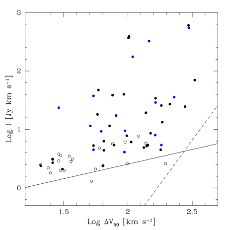
Figure 2: H i   line flux for each galaxy plotted as a function of linewidth measured at the 50% level. Filled dots are confirmed detections; unfilled circles are false detections that were not confirmed in the “pointed” follow-up observations. The solid line indicates the $4~{}\sigma$ detection level. Detections are not expected below the diagonal dashed line at the lower right.

3.2 The Data

3.2.1 Confirmed Detections

The 33 reliable detections are listed in Table 2a. The left-hand part of the table lists the H i   parameters as derived from the driftscan observations. The first column gives the running number of all our 53 galaxy candidates ordered in R.A. The second column gives the the R.A. as explained in section 3 (R.A. = $11^{h}30^{m}+(16\hbox{$.\!\!^{s}$}33\times line)+8^{s}$) and the third column the central declination of the strip on which the signal was detected. Even with the large offset from one declination strip to the next of the Nançay radio telescope (22^′ HPBW), strong sources were, amazingly enough, visible on up to four adjacent strips.

Table 2: a – H i   survey detections and possible detections – reliable detections

— Blind H i   line survey data —								— Possible optical identifications —
No	R.A.	Dec	$V_{\rm HI}$	$W_{50}$	$W_{20}$	$I$	${M}_{\rm HI}$	Ident.	R.A.	Dec	Classif.	$D$	$d$	$mag$	$V_{\rm opt}$
	(1950.0)		km/s	km/s	km/s		${\rm M}_{\odot}$		(1950.0)			′	′		km/s
01	11 36.2	34 05	1852	180	201	4.5	8.56	UGC 6610	11 36 06.0	34 04 58	Scd:	2.1	0.4	15.0	1843
05	11 41.0	31 53	1784	143	152	5.4	8.61	UGC 6684	11 40 43.9	31 43 59	Im?	0.9	0.6	15.07	1794
06	11 53.8	31 31	668	64	76	2.4	7.40	BTS 59	11 53 42	31 34 48	Im/dS0	1.2	0.6	15.5
07	11 56.7	30 47	764	150	178	8.6	8.07	NGC 4020	11 56 22.3	30 41 27	SABd?	2.1	0.9	13.28	778
08	11 59.0	33 43	788	21	63	2.4	7.54	UGC 7007	11 59 00	33 37 10	Scd/Sm:	1.7	1.6	17
09	12 01.6	32 15	743	278	304	24.6	8.50	NGC 4062	12 01 30.5	32 10 26	SA(s)c	4.1	1.7	11.9	742
10	12 06.9	31 09	259	106	116	4.3	6.83	UGC 7131	12 06 39.3	31 11 04	Sdm	1.5	0.4	15.10
11	12 06.9	30 03	614	93	109	40.0	8.55	NGC 4136	12 06 45.3	30 12 21	SAB(r)c	4.0	3.0	11.69	445
		30 25	612	81	100	17.3
12	12 10.0	29 19	1124	164	180	34.2	9.01	NGC 4173	12 09 48.4	29 29 18	Sdm	5.0	0.7	13.59	1121
		29 41	1124	164	225	28.9
13	12 12.4	33 21	1093	212	228	27.1	8.88	NGC 4203	12 12 34	33 28 29	SAB0	3.4	3.2	11.8	1067
14	12 14.4	29 19	1210	70	95	3.6	8.09	UGC 7300	12 14 11.0	29 00 27	Im	1.4	1.2	14.9
15	12 19.3	35 11	732	31	41	2.1	7.42	UGC 7427	12 19 25.9	35 19 41	Im	1.1	0.6	16.5
16	12 19.4	32 15	1134	65	72	6.3	8.28	UGC 7428	12 19 31.8	32 22 09	Im	1.3	1.2	14.1	1193
		32 27	very weak
17	12 21.8	31 53	1240	182	203	25.7	8.97	NGC 4359	12 21 41.8	31 47 56	SB(rs)c?	3.5	0.8	13.40	1199
		31 31	1250	182	201	5.4
18	12 23.2	33 43	310	102	129	389.9	8.95	NGC 4395	12 23 18	33 49	Sd III-IV	13.2	11.0	10.64	311
		34 05	326	109	130	175.1
		33 21	303	95	124	9.5
		34 27	304	94	118	4.1
19	12 24.0	31 31	703	331	377	69.9	8.91	NGC 4414	12 23 57.9	31 30 00	SA(rs)c?	3.6	2.0	10.96	713
22	12 29.6	30 03	654	72	85	11.5	8.06	UGC 7673	12 29 29.0	29 59 06	ImIII-IV	1.4	1.3	15.28
23	12 30.6	31 53	333	59	74	47.3	8.09	UGC 7698	12 30 26.2	31 49 02	Im	6.5	4.5	13.0
		31 31	330	51	73	11.5
26	12 31.5	30 25	1182	140	148	5.2	8.23	NGC 4525	12 31 23.2	30 33 12	Scd:	2.6	1.3	12.88	1163
28	12 35.7	33 21	331	26	35	2.7	7.71	UGCA 292	12 36 13	33 02 29	Im IV-V	1.0	0.7	16.0
		32 59	305	29	44	23.5
29	12 37.4	32 59	760	65	72	4.4	7.78	BTS 147	12 37 43.5	32 55 59	Im	1.2	0.6	15.5
31	12 39.3	32 37	604	296	319	604.1	9.72	NGC 4631	12 39 39.7	32 48 48	SB(s)d	15.5	2.7	9.75	631
		32 59	604	298	317	547.3
		33 21	581	229	285	35.7
32	12 40.9	32 15	666	101	155	369.5	9.59	NGC 4656	12 41 45.4	32 28 43	SBm	15	3	10.8	646
		32 27	623	146	200	324.5
		32 59	637	54	108	37.5
33	12 41.7	34 49	608	58	76	18.1	8.20	UGC 7916	12 42 00	34 39 36	Sm IV	3.9	2.7	14.0
		34 27	605	62	81	9.3
34	12 53.7	34 49	725	54	60	5.3	7.82	UGCA 309	12 53 54	34 55 54	ImIII/N?	1.6	1.4	15.0
35	12 56.4	35 11	848	76	107	38.6	8.82	NGC 4861	12 56 38.5	35 06 56	SB(s)m:	6.1	2.6	12.9	810
		34 49	825	54	71	4.5
36	13 02.8	32 59	889	78	96	5.4	8.00	UGC 8181	13 03 02.9	33 10 02	Sdm	1.5	0.4	16.0
37	13 07.3	34 27	811	138	153	19.3	8.48	UGC 8246	13 07 42	34 27	SB(s)cd	3.5	0.6	14.6
42	13 37.4	31 31	743	26	51	3.1	7.60	UGC 8647	13 37 30.8	31 32 33	Im	1.1	0.3	16.5
47	14 37.4	34 27	1485	185	194	13.3	8.84	NGC 5727	14 38 21.3	34 12 07	SABdm	2.2	1.2	14.2	1523
		34 05	1471	163	178	8.0
48	14 43.0	31 25	1532	98	112	7.8	8.63	UGC 9506	14 43 25.4	31 37 33	Im	0.9	0.4	18
51	14 52.1	31 09	1728	133	157	4.9	8.54	UGC 9597	14 52 53.4	31 01 18	Sm:	1.4	1.1	17
52	14 53.8	30 25	1823	106	128	6.1	8.68	NGC 5789	14 54 28.8	30 26 08	Sdm	0.9	0.8	14.17	1803

Within a declination strip, the H i   parameters were measured from the sum of the lines in which a candidate was detected using the Spectral Line Analysis Package by Staveley-Smith (1985). We list here the heliocentric central line velocity using the optical convention ($V=\frac{c(\lambda-\lambda_{o})}{\lambda_{o}}$), $V_{\rm HI}$, the profile FWHM, $W_{50}$, the profile width measured at 20% of the peak flux density level, $W_{20}$, the integrated line flux, I, and the logarithm of the H i   mass, $M_{\rm HI}$. The latter should be regarded as preliminary as the H i   mass was determined for the strongest appearance of the signal and is uncorrected for the reduction in observed flux (described in section 3.1.) due to offset from the center of the beam. Moreover, the adopted distances were taken straight from the heliocentric H i   velocity $V_{hel}^{\rm HI}$ using a Hubble constant H₀=100 km s^-1 Mpc^-1.

For each H i   detection a possible optical identification is given. Optical redshifts are known for 17 optical candidates, though 30 do have independent H i   velocities (cf., Table 4). The listed optical data are mainly from the NED and LEDA databases; $D$ and $d$ are the optical major and minor axis diameters, respectively, and $V_{\rm opt}$ is the heliocentric optical systemic velocity.

3.2.2 Pointed observations of galaxy candidates

As noted under results, 20 likely detections were identified above the $\approx 4~{}\sigma$ level for which no credible optical counterpart could be identified either in the NED and LEDA databases or by visual examination on the sky surveys. These possible candidates generally are weak ‘signals’ and in order to check on their reality we obtained pointed follow-up observations with the Nançay telescope. These follow-up observations allow the establishment of a database of blind H i   detections in the volume sampled here which is reliable down to the 4 $\sigma$ level. The galaxy candidates are listed in Table 2b with the equivalent parameters as given in Table 2a. Also listed, next to the integrated flux, is the factor above the 1 $\sigma$ noise level to compare it with our 4 $\sigma$ detection limit $I\approx 1.4(\Delta V/30)^{1/2}$ km s^-1 defined in section 3.1.

Table 2: b – Blind H i   survey detections and possible detections – not confirmed by follow-up pointed observations

— Blind H i   line survey data —									— Possible optical identifications —
No	R.A.	Dec	$V_{\rm HI}$	$W_{50}$	$W_{20}$	$I$	$\sigma$	${M}_{\rm HI}$	Identif.	R.A.	Dec	Typ	$D$	$d$	$mag$	$V_{\rm opt}$
	(1950.0)		km/s	km/s	km/s			${\rm M}_{\odot}$		(1950.0)			′	′		km/s
02	11 36.2	33 21	676	99	106	2.6	4	7.45
03	11 38.5	32 37	1835	138	151	5.8	8	8.66	Mk 746	11 38 52.5	32 37 37	Im?	0.4	0.3	15.6	1758
									KUG 1138	11 38 29.5	32 42 15	Im?/Irr	0.4	0.2	15.5	1735
									WAS 28	11 38 59.3	32 33 30	H ii			15.4	1768
04	11 40.7	29 41	380	36	41	2.8	7	6.98
20	12 24.2	31 53	1158	21	40	2.5	10	7.90
21	12 28.9	31 09	1502	52	59	1.3	3	7.61
24	12 30.6	33 43	831	24	33	2.2	7	7.55	MCG 6-29-9	12 30 57	33 37 35	S	1.0	0.3	16
25	12 30.9	32 37	1868	196	206	2.6	3	8.33
27	12 35.5	31 31	185	64	83	2.4	5	6.29
30	12 38.7	32 15	489	30	39	2.0	6	7.05
38	13 14.5	30 03	842	25	35	1.8	8	7.48	CG 0999	13 13 55.9	30 14 25	S01			17.1
39	13 16.7	29 41	2217	60	67	4.8	10	8.74
40	13 18.5	29 19	490	29	61	3.8	11	7.33
41	13 20.8	30 47	1679	32	43	2.0	6	8.12
43	13 46.0	32 59	427	29	39	2.9	8	7.09
44	13 56.4	31 09	168	26	46	3.1	9	6.31
45	14 14.1	31 53	1038	76	92	5.7	10	8.16
46	14 24.7	34 49	1157	121	131	7.7	11	8.38
		or	1201	35	39	3.5	9	8.07
49	14 45.7	31 31	919	95	118	6.1	10	8.10
50	14 45.7	34 49	800	37	42	3.1	8	7.67	UGC 9540?	14 46 48	34 55	triple	1.0	0.3	17
		35 11	801	30	40	3.6	10	7.73
53	15 05.3	33 43	171	56	69	2.1	4	6.16

These follow-up’s resulted in an rms noise of about 6 mJy on average (compared to 10 mJy for the survey). We obtained our observations in total power (position-switching) mode using consecutive pairs of two-minute on- and two-minute off-source integrations. The autocorrelator was divided into two pairs of cross-polarized (H and V) receiver banks, each with 512 channels and a 6.4 MHz bandpass. This yielded a velocity resolution of $\sim$5.2 km s^-1, which was smoothed to 10.5 km s^-1, when required, during the data analysis. The center frequencies of the two banks were tuned to the radial velocity of the galaxy candidate (cf., Table 2b).

The follow-up observations first were repeated on the optimized position from the driftscan detection. If not confirmed, a second round of pointed observations was made, offset by half a beam (11^′) to the north and south of the original position while the original R.A. position which can be determined to higher accuracy was kept constant. In a few cases, a further search at quarter beam offsets was done as well. The follow-up observations consisted of a number of cycles of 2 minutes on- and 2 minutes off-source integration. Off-source integrations were taken at approximately 25^′ east of the target position.

We reduced our follow-up pointed H i   spectra using the standard Nançay spectral line reduction packages available at the Nançay site. With this software we subtracted baselines (generally third order polynomials), averaged the two receiver polarizations, and applied a declination-dependent conversion factor to convert from units of T_sys to flux density in mJy. The T_sys-to-mJy conversion factor is determined via a standard calibration relation established by the Nançay staff through regular monitoring of strong continuum sources. This procedure yields a calibration accuracy of $\sim\pm$15%. In addition, we applied a flux scaling factor of 1.25 to our spectra based on a statistical comparison (Matthews et al. 1998) of recent Nançay data with past observations. The derivation of this scaling factor was necessitated by the a posteriori discovery that the line calibration sources monitored at Nançay by other groups as a calibration normalization check (see Theureau et al. 1997) were very extended compared with the telescope beam, and hence would be subject to large flux uncertainties.

None of the candiates were confirmed, despite the fact that some of them have a rather large mean H i   flux density. Only 4 ‘candidates’ are below our threshold. But, as mentioned above, for the number of independent measurements that were obtained in this survey we expect of the order of 15 positive and 15 negative deviations exceeding $4~{}\sigma$ purely by chance. Many of the “false” detections have very low linewidths (around 30 km s^-1) and could be still be due to radio interference.

The most disappointing candidate was No. 50. This object was identified on two adajcent declination strips and on 2-3 adjacent spectra in R.A. with very consistent H i   properties and a similar high S/N ratio (8 – 10) on both declination strips. It therefore seemed one of the most promising new gas-rich dwarf candidates in the CVn region.

3.2.3 Optically known dwarf galaxies not detected in the survey

Seven dwarf candidates of the BTS survey were not detected in the blind survey. With the exception of BTS 160, these dwarfs were observed individually to a lower sensitivity as the driftscan survey, in the same manner as described in section 3.2.2. We did not include BTS 160, because this dwarf had already been detected by Hoffman et al. (1989) at Arecibo with 0.9 Jy km s^-1. With an average flux density of 26 mJy this dwarf was hence clearly below the threshold of our driftscan survey. Of the 6 remaining dwarfs, none were in fact detected, although the pointed observation of BTS 151 revealed a strong signal with a flux of 20 Jy km s^-1 (cf., values in brackets in Table 3), i.e., a detection which should have popped up as about a 10 $\sigma$ detection in the driftscan mode. However, this signal matches exactly the velocity of the nearby large spiral galaxy NGC 4656 (cf., Table 2a and 4, object No. 32) which is 45^′′ and 17^′ away in R.A. and Dec respectively, hence less than a beamwidth from the pointed observation. The detected signal thus clearly originates from the spiral NGC 4656, and not from the dwarf elliptical BTS 151.

Table 3: Pointed observations BTS dwarfs not detected in the driftscan survey

Ident	R.A.	Dec	Class	$mag$	$D$	Cycl	rms		$V_{\rm HI}$	$W_{50}$	$W_{20}$	$I$	Ref	Tel
							Nan	Are
	(1950.0)				′		mJy	mJy	km/s	km/s	km/s	Jy km/s
BTS 060	11 54 00	30 32 59	dE,N	18.0	0.4	10	3.6
BTS 113	12 15 12	33 36 59	dE/Im	17.5	1.1	17	3.0	1.0
BTS 151	12 41 00	32 45 00	dE	16.0	0.8	8	4.1		[647]	[45]	[80]	[20.0]	*	N
BTS 156	12 46 30	32 14 00	dE	17.0	0.7	8	4.6
BTS 160	12 53 00	33 15 00	Im	15.5	0.7	10	3.6		898	34	58	0.9	H89	A
BTS 161	12 53 42	34 11 00	dE/Im	16.5	0.7	10	3.9	1.1
BTS 167	14 25 00	32 27 00	Im	16.5	0.75	11	3.8

The data of these observatons are summarized in Table 3. Most of these possible dwarf members of the CVn group were not detected in H i  . This supports their classification as early type dwarfs.

3.3 Comparison of driftscan data with pointed observations

Of the 33 reliable detections, 30 galaxies had H i   velocities published in the literature. For the 3 galaxies without prior H i   data we obtained follow-up observations with the Nançay radiotelescope. We also obtained pointed follow-up observations for 8 galaxies already detected before in the H i   line, which seemed to merit an independent, new observation. The observations followed the procedures as described in section 3.2.2.

The results from the driftscan images are summarized in Table 4 together with our new pointed observations and H i   parameters from independent observations.

Table 4: Comparison of survey data with pointed H i   line observations

		— H i   survey data —						— pointed H i   observations —
No	Identif.	Dec	$V_{\rm HI}$	$W_{50}$	$W_{20}$	$I$	${M}_{\rm HI}$	$V_{\rm HI}$	$W_{50}$	$W_{20}$	$I$	Ref	Tel
			km/s	km/s	km/s	Jy km/s	${\rm M}_{\odot}$	km/s	km/s	km/s	Jy km/s
01	UGC 6610	34 05	1852	180	201	4.5	8.56	1851	209	222	8.8	$\ast$	N
								1851	20	211	9.2	B92	N
05	UGC 6684	31 53	1784	143	152	5.4	8.84	1788	142	159	5.8	S90	A
								1789	108	161	6.5	TS79	G
06	BTS 59	31 31	668	64	76	2.4	7.40	648	48	65	7.1	H89	A
07	NGC 4020	30 47	764	150	178	8.6	8.07	760	162	183	11.1	S90	A
								757	175	193	13.3	FT81	E
								760		180		G94	E
								762	176		9.1	M94	A
08	UGC 7007	33 43	788	21	63	2.4	7.54	771	59	70	2.5	$\ast$	N
								774		72	3.4	TC88	G
								786		67	3.8	FT81	G
09	NGC 4062	32 15	743	278	304	24.6	8.50	774	303	298	17.3	DR78	G
								769	312	307	26.7	FT81	G
								766		356	24.8	DS83	G
								765	288	303	19.5	HS85	E
								767		310	23.6	H83	A
								774				RD76	G
								764	302	303	25.1	BW94	W
								779	325	315	41.7	F95	A
10	UGC 7131	31 09	259	106	116	4.3	6.83	253	117	128	4.6	S90	A
								249				B85b	A
11	NGC 4136	30 03	614	93	109	40.0	8.85	606	85	104	32.1	$\ast$	N
		30 25	612	81	100	17.3		618	94	112	49.4	FT81	G
								612	89	107	47.1	HR86	E
								606	92	109	25.0	L87	A
								596	101	128	35.0	A79	Cambr
								607		105		G94	E
12	NGC 4173	29 19	1124	164	180	34.2	9.01	1122	158	172	33.0	$\ast$	N
		29 41	1124	164	225	28.9		1127	170	205	42.2	FT81	G
								1020	58	98	21.6	WR86	A
								1085	83	150	19.7	B85	A
								1127		173		G94	E
13	NGC 4203	33 21	1093	212	228	27.1	8.88	1080	230	270	6.4	BB77	A
								1083		264	26.7	BC83	N
								1091	240		27.4	B87	A
								1093	229	274	20.7	K77	B
								1091			27.1	BK81	A
								1091	240		27.6	B87	A
								1094		265		G94	E
								1090	243	283	24	vD88	W
14	UGC 7300	29 19	1210	70	95	3.6	8.09	1210	73	91	10.4	S90	A
								1224	70	96		TW79	A
								1215	78	102	13.1	FT81	G
								1208		98		G94	E
								1210	75		13.8	VZ97	B
15	UGC 7427	35 11	732	31	41	2.1	7.42	719	35	72	0.8	$\ast$	N
								724	41	61	2.8	S90	A
								725	39	57	2.3	H89	A
								729				B85b	A
16	UGC 7428	32 15	1134	65	72	6.3	8.28	1138	67	83	9.2	$\ast$	N
		32 37	very weak					1137	66	85	7.3	S90	A
								1140	65	83	7.6	L87	A
17	NGC 4359	31 53	1240	182	203	25.7	8.97	1253	204	220	22.3	FT81	E
		31 31	1250	182	201	5.4				216		G94	E
18	NGC 4395	33 43	310	102	129	389.9	8.95	320		140	300	R80	G
		34 05	326	109	130	175.1		318	112	132	330.2	HS85	E
		33 21	303	95	124	9.5		315	101	141	176.8	DR78	G
		34 27	304	94	118	4.1		318	123	135	334.3	FT81	B
								330	118	135	296.7	W86	W
								319			405.8	H98	B
19	NGC 4414	31 31	703	331	377	69.9	8.91	720	380	418	65.1	FT81	G
								716	383	422	63.1	RA86	W
20	UGC 7673	30 03	654	72	85	11.5	8.06	639	55		8.9	FT75	G
								639	58	73	9.2	FT81	G
								643		91	9.6	TC88	G
								645	70		14.0	H96	A
								649	61	82	6.7	H89	A
								644		86		G94	E
								644	72		10.4	VZ97	B
								642				B85b	A
21	UGC 7698	31 53	333	59	74	47.3	8.09	335	63		35.0	FT75	G
		31 31	330	51	73	11.5		331		73	41.1	TC88	G
								335	66	93	43.1	FT81	B
								332	55	72	52.2	H81	E
								334	53	72	17.9	H89	A
								331			41.0	H98	B
								334	48	76	29.9	A79	Camb
26	NGC 4525	30 25	1182	140	148	5.2	8.23	1165	145	164	6.3	$\ast$	N
								1174		162		G94	E
								1177	149	161	6.7	T98	N
								1172	149		6.5	K96	W
28	UGCA 292	32 59	305	29	44	23.5	7.71	309	29	42	13.9	$\ast$	N
		33 21	331	26	35	2.7		312		51	13.6	FT81	G
								308		44	11.0	TC88	G
								307	25			LS79	E
								309	30		20.5	H96	A
								308	27		15.7	VZ97	B

Table 4: Comparison of survey data with pointed H i   line observations – continued

		— H i   survey data —						— pointed H i   observations —
No	Identif.	Dec	$V_{\rm HI}$	$W_{50}$	$W_{20}$	$I$	${M}_{\rm HI}$	$V_{\rm HI}$	$W_{50}$	$W_{20}$	$I$	Ref	Tel
			km/s	km/s	km/s	Jy km/s	${\rm M}_{\odot}$	km/s	km/s	km/s	Jy km/s
29	BTS 147	32 59	760	65	72	4.4	7.78	765	58	90	3.8	H89	A
								775			5.5	R94	W
31	NGC 4631	32 37	604	296	319	604.1	9.72	617	286	320	323.6	DR78	G
		32 59	604	298	317	547.3		613		320	639.3	R80	G
		33 21	582	229	285	35.7		600			610	W69	N
								613	301	325	604.3	FT81	B
								606	261	306	787.6	KS77	A
								606				KS79	A
								610		380	506.1	W78	W
								615			428.8	R94	W
											766.1	H75	E
32	NGC 4656	32 15	666	101	155	369.5	9.59	645	126	194	182.3	DR78	G
		32 27	623	146	200	324.5		644		174	393.0	R80	G
		32 59	637	54	108	37.5		639		212	305.9	DS83	G
								646		184	274.6	TC88	G
								649	146	187	327.0	FT81	B
								630			258	W69	N
								650		240	265.6	W78	W
								634				KS79	A
								660			302.2	R94	W
33	UGC 7916	34 49	608	58	76	18.1	8.20	603		81	18.3	TC88	G
		34 27	605	62	81	9.3		612	60	87	25.4	FT81	B
								603	57	77	10.5	H89	A
34	UGCA 309	34 49	725	54	60	5.3	7.82	731		53	5.8	TC88	G
								730	57	67	7.0	FT81	G
								717	40		6.4	LS79	E
								730	42		5.6	VZ97	B
35	NGC 4861	35 11	848	76	107	38.6	8.82	839	89	118	34.3	$\ast$	N
		34 49	825	54	71	4.5		837		119	39.5	C74	N
								847		114	49.1	BC81	N
								847	86	116	40.6	FT81	G
								843	150	215	56.5	B82	N
								839	87	110	34.1	BW94	W
36	UGC 8181	32 59	889	78	96	5.4	8.00	894	104	146	4.4	$\ast$	N
								886	97	115	4.0	S90	A
								882				B85b	A
37	UGC 8246	34 27	811	138	153	19.3	8.48	813	138	170	19.7	FT81	G
								749				B85b	A
42	UGC 8647	31 31	743	26	51	3.1	7.60	747	47	77	5.1	S90	A
47	NGC 5727	34 27	1485	185	194	13.3	8.84	1489		217	15.1	H83	G
		34 05	1471	163	178	8.0		1491	192	196	13.6	FT81	G
								1492		202	15.1	HG84	A
48	UGC 9506	31 25	1532	98	112	7.8	8.63	1530	61	119	6.9	$\ast$	N
								1519	51	102	4.1	S90	A
								1521		120	8.0	TS79	G
51	UGC 9597	31 09	1728	133	157	4.9	8.80	1734	135	150	3.1	S90	A
								1727	128	200	5.3	TS79	G
52	NGC 5789	30 25	1823	106	128	6.1	8.68	1800	118	190	8.0	P79	G
								1801		165	6.9	TC88	G
								1806	96	133	5.8	OS93	W
								1805	105		5.9	C93	A

Table 4: References and Telescope Codes

A79	Allsopp (1979)	BC81	Balkowski & Chamaraux (1981)	BC83	Balkowski & Chamaraux (1983)
BB77	Bieging & Biermann (1977)	B85	Bothun et al. (1985)	B85b	Bothun et al. (1985b)
B82	Bottinelli et al. (1982)	B92	Bottinelli et al. (1992)	BW94	Broeils & van Woerden (1994)
BK81	Burstein & Krumm (1981)	B87	Burstein et al. (1987)	C74	Carozzi et al. (1974)
C93	Chengalur et al. (1993)	DS83	Davis & Seaquist (1983)	DR78	Dickel & Rood (1978)
FT75	Fisher & Tully (1975)	FT81	Fisher & Tully (1981)	F95	Freudling (1995)
G94	Garcia-Baretto et al. (1994)	HG84	Haynes & Giovanelli (1984)	H98	Haynes et al. (1998)
H83	Hewitt et al. (1983)	H89	Hoffman et al. (1989)	H96	Hoffman et al. (1996)
H75	Huchtmeier (1975)	H81	Huchtmeier et al. (1981)	HS85	Huchtmeier & Seiradakis (1985)
HR86	Huchtmeier & Richter (1986)	K96	Kamphuis et al. (1996)	K77	Knapp et al. (1977)
KS77	Krumm & Salpeter (1977)	KS79	Krumm & Salpeter (1979)	L87	Lewis (1987)
LS79	Lo & Sargent (1979)	M94	Magri (1994)	OS93	Oosterloo & Shostak (1993)
P79	Peterson (1979)	R94	Rand (1994)	RA86	Rhee & van Albada (1996)
RD76	Rood & Dickel (1976)	R80	Rots (1980)	S90	Schneider et al. (1990)
TW79	Tarter & Wright (1979)	T98	Theureau et al. (1998)	TS79	Thuan & Seitzer (1979)
TM81	Thuan & Martin (1981)	TC88	Tifft & Cocke (1988)	vD88	van Driel et al. (1988)
VZ97	Van Zee et al. (1997)	W69	Weliachew (1969)	W78	Weliachew et al. (1978)
W86	Wevers et al. (1986)	WR86	Williams & Rood (1986)	$\ast$	this paper
A	Arecibo	B	Green Bank 43-m.	E	Effelsberg
G	Green Bank 90-m.	N	Nancay

Overall, the agreement between the measurements obtained from the driftscan survey and independent pointed observations are very satisfactory with a few discrepancies discussed below:

No. 12 (NGC 4173): The H i   line parameters of this 5^′ diameter edge-on system measured at Arecibo by Williams & Rood (1986) and independently by Bothun et al. (1985) are quite different from the other available values.

No. 13 (NGC 4203): This lenticular galaxy has an optical inclination of about 20^∘. Assuming that the gas rotates in the plane of the stellar disk, very high H i   rotational velocities would be derived. However, radio synthesis imaging (van Driel et al. 1988) has shown that the outer gas rotates in a highly inclined ring at an inclination of about 60^∘, the value adopted in correcting the profile widths (see Table 5).

For 4 galaxies (No. 33 = UGC 7916, No. 34 = UGCA 309, No. 35 = NGC 4861, No. 38 = CGCG 0999) the listed properties such as morphological type, diameters and magnitudes differ between the LEDA and NED. The values in Table 2b and Table 5 are from LEDA.

We have compared the systemic velocities, line widths, integrated line fluxes and H i   masses of the 33 reliable survey detections with available pointed observations. It should be noted that the comparison data represent in no way a homogeneous set of measurements, as they were made with various radio telescopes throughout the years; especially, care should be taken that no H i   flux was missed in observations with the $3^{\prime}\,.8$ round Arecibo beam.

A comparison of the difference between systemic velocities (actually, the centre velocities of the line profiles) measured at Nançay and elsewhere shows no significant dependence on radial velocity, with the exception of one data point for NGC 4173 (No. 12). Here we consider the radial velocity of 1020 km s^-1 measured at Arecibo by Williams & Rood (1986) as spurious, seen the agreement between the 3 other measured values. The mean value and its standard deviation of the Nançay–others systemic velocity difference is 0.8$\pm$11.7 km s^-1 (for a velocity resolution of 10.2 km s^-1 at Nançay).

A comparison of the difference between the $W_{50}$ and $W_{20}$ H i   line widths measured at Nançay and elsewhere shows a good correlation as well; the largest discrepancy is found between the survey values for the 5^′ diameter edge-on system NGC 4173 (No. 12) and the Arecibo $W_{50}$ and $W_{20}$ measurements by Williams & Rood (1986) as well as by Bothun et al. (1985), while the other pointed observations of this object are consistent with ours.

A comparison of the difference between the integrated H i   line fluxes measured in the Nançay survey and elsewhere shows a reasonable correlation. This indicates that the assumption of a constant (uncalibrated) system temperature of 50 K throughout the survey is justified. 3 larger discrepancies occur. This concerns No. 13 = NGC 4203 for which the Nançay survey flux is considerably higher than the flux measured at Arecibo. As the galaxy’s outer H i   ring is much larger than the Arecibo beam (see van Driel et al. 1988) the Nançay measurement will reflect tht total flux. For No. 06 = BTS59 and No. 14 = UGC 7300, the Nançay flux is also considerably higher than a flux measured at Arecibo by Hoffman et al. (1989) , respectively Schneider et al. (1990); both are objects of about $1^{\prime}\,.2$ optical diameter only.

A comparison between the H i   masses derived straight from the detections in the strip-images with pointed observations shows an astonishingly narrow correlation from the lowest to the highest H i   masses detected in this survey. Overall, only a slight offset towards lower masses is noticeable for the driftscan results compared to pointed observations. This obsviously is due to the fact that the driftscan detects the galaxies at various offsets from the center of the beam.

4 Discussion

4.1 Properties of the detected galaxies

We derived a number of global properties for the 33 galaxies with reliable detections in our H i   line survey based on the available pointed H i   data, including our own new results. These are listed in Table 5. The values for the observed linewidths and the heliocentric velocity are the means from all individual pointed observations listed in Table 4. The inclination, i, is derived from the cosine of the ratio of the optical minor and major axis diameters, the profile widths $W_{50}$ and $W_{20}$ were corrected to $W_{50}^{cor}$ and $W_{20}^{cor}$, respectively, using this inclination. The H i  -mass and blue absolute magnitude, $M_{\rm B}$, were as a first approximation computed straight from the observed velocity and a Hubble constant of $H_{o}=100$ km s^-1 Mpc^-1. We furthermore assumed that all apparent magnitudes listed in Table 2 were measured in the B band.

Table 5: H i   properties of galaxies detected in the drift-scan CVn galaxy search

No	Ident.	Class.	$i$	$W_{50}$	$W_{20}$	$W_{50}^{\rm cor}$	$W_{20}^{\rm cor}$	$V_{\rm HI}$	${M}_{\rm HI}$	$M_{\rm B}$	$V_{\rm HI}^{\rm POT}$	${M}_{\rm HI}$POT	$M_{\rm B}^{\rm POT}$	${M}_{\rm HI}$/$L_{\rm B}$
			∘	km/s	km/s	km/s	km/s	km/s	${\rm M}_{\odot}$	mag	km/s	${\rm M}_{\odot}$	mag	${\rm M}_{\odot}$/$L_{\odot,{\rm B}}$
01	UGC 6610	Scd:	79	207	216	210	220	1851	8.86	-16.3	2396	9.08	-16.5	1.41
05	UGC 6684	Im?	48	125	160	168	215	1789	8.67	-16.1	2316	8.89	-16.3	1.09
06	BTS 59	Im/dS0	60	48	65	55	75	648	7.85	-13.6	976	8.21	-14.0	1.65
07	NGC 4020	SABd?	65	171	185	188	204	760	8.18	-16.1	1103	8.50	-16.4	0.35
08	UGC 7007	Scd/Sm:	20	59	70	172	205	777	7.66	-12.4	1137	7.99	-12.7	3.22
09	NGC 4062	SA(s)c	65	306	313	337	345	770	8.55	-17.4	1118	8.87	-17.7	0.25
10	UGC 7131	Sdm	74	117	128	121	133	251	6.83	-11.9	487	7.41	-12.5	0.76
11	NGC 4136	SAB(r)c	41	92	111	140	169	608	8.51	-17.2	906	8.86	-17.5	0.27
12	NGC 4173	Sdm	82	117	160	118	162	1096	8.91	-16.6	1479	9.17	-16.9	1.20
13	NGC 4203	SAB0	20	236	271	690	792	1089	8.85	-18.3	1489	9.12	-18.6	0.22
14	UGC 7300	Im	31	74	97	143	188	1213	8.63	-15.5	1607	8.87	-15.7	1.73
15	UGC 7427	Im	57	38	63	45	75	724	7.39	-12.8	1061	7.72	-13.1	1.20
16	UGC 7428	Im	23	66	84	168	215	1138	8.39	-16.1	1531	8.65	-16.4	0.57
17	NGC 4359	SB(rs)c?	23	204	218	522	558	1253	8.92	-17.0	1658	9.16	-17.2	0.85
18	NGC 4395	Sd III-IV	34	113	137	202	245	320	8.87	-16.8	569	9.37	-17.3	0.91
19	NGC 4414	SA(rs)c?	56	382	420	460	507	718	8.89	-18.2	1027	9.20	-18.5	0.26
22	UGC 7673	ImIII-IV	22	63	83	168	222	643	7.98	-13.7	923	8.29	-14.0	2.03
23	UGC 7698	Im	46	57	77	79	107	333	8.00	-14.6	567	8.46	-15.1	0.93
26	NGC 4525	Scd:	60	148	162	170	187	1172	8.32	-17.4	1545	8.56	-17.6	0.15
28	UGCA 292	Im IV-V	46	28	46	38	64	309	7.53	-11.4	542	8.02	-11.9	6.00
29	BTS 147	Im	60	58	90	66	104	770	7.82	-13.9	1082	8.12	-14.2	1.17
31	NGC 4631	SB(s)d	80	283	330	287	335	610	9.71	-19.1	891	10.04	-19.4	0.76
32	NGC 4656	SBm	78	136	199	139	203	644	9.45	-18.2	927	9.77	-18.5	0.95
33	UGC 7916	Sm IV	46	59	82	82	114	606	8.19	-14.9	894	8.53	-15.2	1.09
34	UGCA 309	ImIII/N?	29	46	60	94	124	727	7.89	-14.3	1025	8.19	-14.6	0.95
35	NGC 4861	SB(s)m:	65	103	132	113	146	842	8.85	-16.7	1157	9.13	-17.0	0.95
36	UGC 8181	Sdm	74	101	131	105	136	887	7.89	-13.7	1190	8.15	-14.0	1.65
37	UGC 8246	SB(s)cd	80	138	170	140	173	781	8.45	-14.9	1070	8.72	-15.2	1.99
42	UGC 8647	Im	74	45	77	46	80	747	7.83	-12.8	982	8.07	-13.0	3.30
47	NGC 5727	SABdm	57	192	208	228	248	1491	8.89	-16.6	1748	9.03	-16.7	1.14
48	UGC 9506	Im	64	56	114	62	127	1523	8.54	-12.9	1767	8.67	-13.0	15.42
51	UGC 9597	Sm:	38	132	175	214	284	1730	8.47	-14.1	1973	8.58	-14.2	4.35
52	NGC 5789	Sdm	27	106	163	233	359	1803	8.71	-17.1	2047	8.82	-17.2	0.48
Note: For comments on the inclination of the H i   gas in NGC 4203 (no. 15), see Sect 4.3

The survey region lies quite close in the sky to the Virgo cluster. This is illustrated in Fig. 3 which shows the Nançay survey region in Supergalactic coordinates, with the positions of the in H i   detected galaxies as well as the apex of the Virgocentric flow field, M87. The proximity of our survey region to the Virgo overdensity motivated us to calculate distances to our galaxies using the POTENT program (Bertschinger et al. 1990), hence corrected for Virgocentric infall.

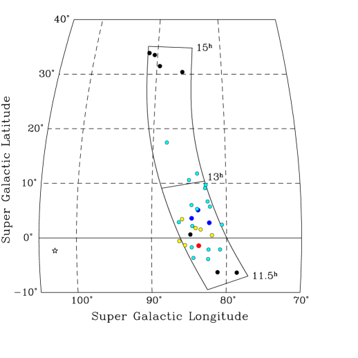
Figure 3: Location of the detected galaxies in Supergalactic coordinates. The survey area is bounded by solid lines; the beginning R.A. at 11.5^h and ending R.A. at 15^h are marked. The star symbol at the lower left indicates the position of Virgo A$=$M87.

The POTENT corrections are based on the overall underlying density field deduced from flow fields out to velocities of 5000 km s^-1. A comparison of the correction with a pure Virgocentric infall model (cf., Kraan-Korteweg 1986) confirms that the main perturbation of the velocity field within our survey region is due Virgocentric infall. More local density fluctuations or a Great Attractor component (at an angular distance of $\approx$ 77) have little impact on the velocities.

The “absolute” corrections to the observed velocity due the Virgo overdensity vary depending on velocity and angular distance from the Virgo cluster. But the effects on global properties such as magnitudes and luminosities and H i  -masses can be quite significant, particularly for low velocity galaxies at small angular distance from the apex of the streaming motion (Kraan-Korteweg 1986).

The for streaming motions corrected velocities, absolute magnitudes and H i  -masses based on POTENT distances are also listed in Table 5. The corrections in velocity reach values of nearly a factor of 2, the respective corrections in absolute magnitudes of $0\hbox{$.\!\!^{m}$}6$ and the logarithm of the H i  -masses of up to 0.6 dex.

In Fig. 4 the measured velocity width is plotted as a function of H i   mass. There is a well known trend (a sort of H i   Tully-Fisher Relation) that larger $M_{HI}$ masses are strongly correlated with higher rotation speeds (cf., Briggs & Rao 1993). Fig. 4 displays H i  -masses based on observed velocities as well as H i  -masses corrected for Virgocentric flow using the POTENT program (solid respectively open circles) including the shifts in galaxy masses due to the perturbed velocity field. The drawn line indicates an upper bound to the velocity width, based on disk galaxies that are viewed edge-on; galaxies falling far below the line are viewed more face-on.

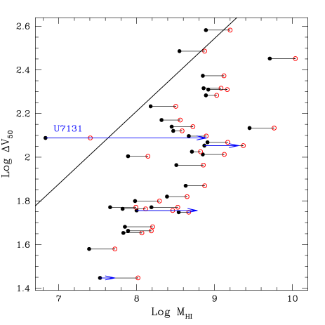
Figure 4: Log of velocity width (50%) as a function of H i   mass, $M_{HI}$, for the confirmed detections. The line is a boundary to the H i  -mass versus line-width relation derived from a much larger sample of galaxies (Briggs & Rao 1993), $\Delta V=0.35(M_{HI}/M_{\odot})^{1/3}$ km s^-1. H i   masses computed using distance $d=v_{hel}/H_{o}$ are marked by solid dots. Open circles mark masses corrected to POTENT distances to compensate for Virgocentric flow, and the arrows indicate the masses for galaxies with independent distance measures as referenced in the text.

A surprise that appeared in Fig. 4 is that one galaxy, UGC 7131, from our Nançay survey lies above the usual bound for velocity width, even after correction for Virgocentric infall.

Subsequently, new measurements of distance using resolved stellar populations were released for four of our galaxies (Karachentsev & Drozdovsky 1998, Marakova et al. 1998). This includes UGC 7131, which was found to lie at a distance $d>14$ Mpc, i.e., considerably further than indicated from the observed velocity listed in Table 5 ($V^{hel}=251~{}\mbox{\rm km\,s${}^{-1}$}$) or for flow motions corrected velocity ($V^{POT}=487~{}\mbox{\rm km\,s${}^{-1}$}$). However, with this new independent distance estimate UGC 7131 does fall within the H i  -mass range expected for its linewidth.

Its morphology as evident on the sky survey plates does not indicate a morphology earlier than the galaxy type listed in Table 2a of Sdm for which one could expect a higher H i  -mass in agreement with its new determination (cf., shift in Fig. 4). It has a slight comet-like structure not atypical for BCD galaxies. On the other hand, the deep CDD-image in Markarova et al. (1998, their Fig. 3) finds UGC 7131 to be unresolved and amorph, which does confirm the larger distance and is not consistent with a nearby (low–velocity) galaxy.

Interestingly enough, the angular distance is a dominant parameter on the infall pattern. UGC 7131 has a very small angular distance from the Virgo cluster, i.e., only 19 degrees. If it were at a slightly smaller angle, and depending on the model parameters for the virgocentric model, the solution for the distance would become triple valued: typically with one solution at low distance, one just in front of the Virgo cluster distance, and one beyond the Virgo cluster distance (cf., Fig. 3 in Kraan-Korteweg 1986). Although the angular distance (from the Virgo cluster core) within which we find triple solutions does depend on the infall parameters such as the decleration at the location of the Local Group, none of the models with currently accepted flow field parameters suggests a triple solution for galaxies with observed velocities as low as the one measured for UGC 7131, except if the density profile within the Virgo supercluster were considerably steeper than usually assumed.

With the exception of the observed velocity, all further indications about UGC 7131 support the considerably larger distance — even its distribution in redshift space. The locations of the H i   selected galaxies are shown in a cone diagram in Fig. 5 with the radial coordinate of Heliocentric velocity and where the POTENT distances are drawn as contours. An arrow indicates the revision with regard to the location of UGC 7131. It is clear from this display that UGC 7131 is not a member of the nearby CVn I group, nor of the more distant CVn II group, but most likely is a member of the Coma I group. (Since our distances and survey volumes have been computed for convenience using $H_{o}=100$ km s^-1 Mpc^-1, the distances for these four galaxies were adjusted to our scale, assuming that they were correct in a system with $H_{o}=75$ km s^-1 Mpc^-1.)

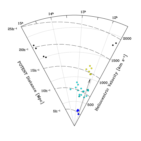
Figure 5: Cone diagram showing the relative locations of the detected galaxies as a function of R.A. and heliocentric redshift in km s^-1. Long dashes show contours of constant distance computed using POTENT (Bertschinger et al. 1990) to compensate for Virgocentric flow. The arrow indicates the revised distance for UGC 7131 (Karachentsev & Drozdovsky 1998).

Assuming that both the observed velocity and the revised distance to UGC 7131 are correct, this can only be combined if this galaxy resides in a triple solution region of the Virgocentric flow pattern, implying that our current knowledge of the density field within the Local Supercluster and the induced flow motions are not yet well established. On the positive side, this example demonstrates that independent distance derivations of fairly local galaxies, close in the sky to the Virgo, can teach us considerably more about the density field and the flow patterns within the Local Supercluster.

4.2 Comparison with the F-T Catalog

A convenient plot for comparing relative sensitivities of different surveys, such as the Fisher-Tully Catalog of Nearby (late-type) Galaxies (1981b) and the more recent LSB catalogs (Schombert et al. 1997, Sprayberry et al. 1996) is shown in Fig. 6. Here, the distance to each galaxy is plotted as a function of its H i   mass. Briggs (1997a) showed that there is a sharp sensitivity boundary to the Fisher-Tully catalog, indicated by the diagonal dashed line in Fig. 6, and that the newer surveys for LSB galaxies add no substantial number of objects to the region where Fisher-Tully is sensitive. The new objects lie predominantly above the F-T line. A crucial test provided by the new Nançay survey, is to cover a large area of sky at a sensitivity matched to the Fisher-Tully sensitivity, to determine whether their catalog is indeed complete. The result shown in Fig. 6 is that the Nançay survey finds galaxies both within the F-T zone and above it. All the galaxies that we detected within the F-T intended “zone of completeness” (below their sensitivity line and within 10$h^{-1}$Mpc) were already included in the F-T Catalog. One notable galaxy that was not included in the F-T Catalog, NGC 4203, lies well within the F-T zone of sensitivity; it is classified Hubble type S0 and therefore was not included in Fisher and Tullys’ source list of late-type galaxies. We conclude that the F-T Catalog is remarkably complete in this region for late-type galaxies, and that the biggest incompleteness that may arise when their catalog is used for measuring the H i   content of the nearby universe is that the F-T Catalog may be lacking the occasional early-type galaxy with substantial H i  .

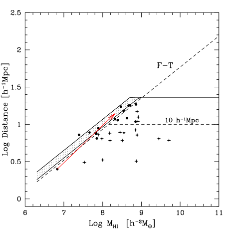
Figure 6: Distance to each of the detected galaxies plotted as a function of HI-mass, $M_{HI}$. Plus symbols indicate objects detected by Fisher & Tully (1981b); solid dots are for objects that were not. The arrow indicates the shift implied for the revised distance to the galaxy UGC 7131 (Makarova et al. 1998). A diagonal line indicates the sensitivity attained by the Fisher-Tully Catalog (1981b), as estimated by Briggs (1997). The cross-hatched band indicates the range of the $4~{}\sigma$ level, depending on the coordinates of the galaxies relative to the center of the survey strip.

4.3 The H i  -mass function

The distribution of H i  -masses is rather homogeneous with a mean of log($M_{HI}$) = 8.4 for observed velocities – and of log($M_{HI}$) = 8.7 for POTENT corrected HI-masses. An HI-mass function can be estimated in a straightforward way for our Nançay sample. The precision of this computation will be low for several reasons: The total number of galaxies is low. There are no masses below $M_{HI}\approx 3{\times}10^{7}M_{\odot}$. The volume scanned is small, and it cannot be argued that the sample is drawn from a volume that is respresentative of the general population, in either H i   properties or in the average number density. However, the calculation is a useful illustration of the vulnerability of these types of calculation to small number statistics and distance uncertainties.

We show four derivations of the H i   mass function in Fig. 7. First, we calculated the number density of galaxies by computing distances, H i   masses, and sensitivity volumes based on heliocentric velocities $V_{hel}/H_{o}$. The mass functions are binned into half-decade bins, but are scaled to give number of objects per decade. The value for each decade is computed from the sum $\Sigma 1/V_{max}$, where $V_{max}$ is the volume of the survey in which a galaxy with the properties $M_{HI}$ and $\Delta V$ could have been detected. The values of $1/V_{max}$ are plotted for every galaxy as dots. The points representing the number density of objects of mass $M_{HI}$ are plotted per bin at the average $M_{HI}$ for the galaxies included in that bin, so that, for example, the two highest mass bins, which have only one galaxy each, are plotted close to each other as upper limits. It is notable that the galaxy UGC 7131 causes a very steeply rising tail in the top panel, because is is treated in this calculation as a very nearby, but low mass object. Placed at a greater, more appropriate distance, it becomes more massive, and it is added to other galaxies of greater velocity width and higher H i   mass in the higher mass bins.

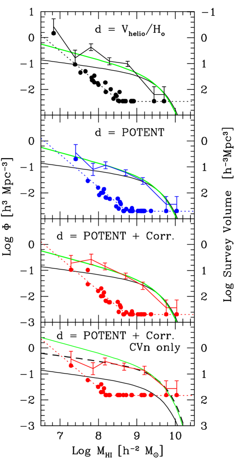
Figure 7: HI-mass function for the Canis Venatici survey volume, normalized to number of objects per decade of mass. Error bars represent poisson statistics for the present sample after binning. The smooth solid curve is the analytic form derived by Zwaan et al. (1997) with a slope of $\alpha=-1.2$, the grey line has a slope of $\alpha=-1.4$ (Banks et al. 1998). The bottom panel shows the result restricted to the CVn-group regions ($<$1200km s^-1) where the dashed curve represents the Zwaan et al. H i  -mass function multiplied by a factor of 4.5. The dotted line gives an indication of the volume probed as a function of mass (see right vertical axis); the points give $1/V_{max}$ for each of the galaxies in the sample, taking into account the different velocity widths.

An improved calculation based on the POTENT distances is displayed in the second panel. In the third panel, the four galaxies with independent distance measurements have been plotted according to their revised distances. In the 4th panel we have restricted our sample to include only the overdense foreground region which includes the CVn and Coma groups, i.e., the volume within $V_{hel}<$1200km s^-1 and about 1/2 the RA coverage (about half the solid angle). Big galaxies can be detected throughout the volume we surveyed, but little galaxies can be detected only in the front part of our volume. The volume normalization factors, which are used to compute the mass function, are sensitivity limited for the small masses to only the front part of our survey volume. For the large masses, the $V_{max}$’s include the whole volume, including the volume where the numbers of galaxies are much less. Hence, when restricting the “survey volume” we get a fairer comparison of the number of little galaxies to the number of big ones.

In all four panels the solid line represents the H i  -mass function with a slope of $\alpha=-1.2$ as derived by Zwaan et al. (1997) from the Arecibo blind H i   driftscan survey, whereas the grey line represents an H i  -mass function with a slope of $\alpha=-1.4$ as deduced by Banks et al. (1998) for a similar but more sensitive survey in the CenA-group region.

In the first three panels, the steeper slope seems to be in closer agreement with the survey results than the more shallow H i  -mass function with $\alpha=-1.2$. However, as argued above, the small masses are over-represented in comparison to the large masses if we regard the full Nançay survey region. This leads to a slope that is too steep for the faint end. Restricting our volume to the dense foreground region including “only” the CVn and Coma groups, we find that the Zwaan et al.  H i  -mass function with a scaling factor of 4.5 to acount for the local overdensity (dashed line in the bottom panel) gives an excellent fit to the data.

5 Conclusion

The principal conclusion from this survey is that no new HI-rich systems (LSB galaxies or intergalactic clouds) were discovered. The previous deep optical surveys in the CVn group region (BTS), followed by 21cm line observations, have succeeded in cataloging all the galaxies that the current Nançay survey detected. With the follow-up observations (and their non-confirmations) of all $4~{}\sigma$ events, the survey is complete to H i   masses above $8{\times}10^{7}M_{\odot}$ throughout the CVn Groups. This limit is most strict for the high mass range. This corroborates the early conclusions made by Fisher and Tully in 1981(a) from their blind H i  -survey in the M81-group region with a limiting sensitivity a factor two higher compared to the here performed H i  -survey.

The logical consequence is that intergalactic clouds and unseen gas-rich galaxies can form a population amounting to at most 1/30 the population in optically cataloged large galaxies. This result is highly consistent with earlier work (Zwaan et al. 1997, Briggs 1997b, Briggs 1990).

For lower H i   masses, the current Nançay Survey was insufficiently sensitive for detections throughout the groups. The depth of the experiment drops as $d\approx 12(M_{HI}/10^{8}\mbox{${\rm M}_{\odot}$})^{5/12}h^{-1}$kpc, so that the volume in which small masses ($M_{HI}\mathrel{\hbox{\hbox to0.0pt{\hbox{\lower 4.0pt\hbox{$\sim$}}\hss}\hbox{$<$}}}10^{8}M_{\odot}$) could be detected is small and does not extend to include both CVn Groups.

The H i  -defined sample obtained here, which is complete to $8{\times}10^{7}M_{\odot}$ throughout the CVn and Coma groups is well described by the Zwaan et al. (1997) H i  -mass function with a slope of $\alpha=-1.2$ and a scaling factor of 4.5.