The enhancement and decrement of the Sunyaev-Zeldovich effect
towards the ROSAT Cluster RXJ0658-5557

Abstract

We report simultaneous observations at $1.2$ and $2\,$mm, with a double channel photometer on the SEST Telescope, of the X-ray cluster RXJ0658-5557 in search for the Sunyaev-Zel’dovich (S-Z). The S-Z data were analyzed using the relativistically correct expression for the Comptonizationand we find from the detected decrement $(2.60\pm 0.79)~{}10^{-4}$, which is consistent with that computed using the X-ray (ROSAT and ASCA) observations. The uncertainty includes contributions due to statistical uncertainty in the detection and systematics and calibration. The 1.2 mm channel data alone gives rise to a larger Comptonization parameter and this result is discussed in terms of contamination from foreground sources and/or dust in the cluster or from a possible systematic effect. We then make use of the combined analysis of the ROSAT and ASCA X-ray satellite observations to determine an isothermal model for the S-Z surface brightness. Since the cluster is asymmetrical and probably in a merging process, models are only approximate. The associated uncertainty can, however, be estimated by exploring a set of alternative models. We then find as the global uncertainty on the Comptonization parameter a factor of 1.3. Combining the S-Z and the X-ray measurements, we determine a value for the Hubble constant. The 2 mm data are consistent with $H_{0}(q_{0}=\frac{1}{2})=53^{+38}_{-28}\,{\rm kms}^{-1}{\rm Mpc}^{-1}$, where the uncertainty is dominated by the uncertainty in models of the X-ray plasma halo.

1 INTRODUCTION

The inverse Compton scattering on the photons of the Cosmic Microwave Background (CMB) by the hot e^- gas residing in rich clusters of galaxies causes an effect known as the Sunyaev-Zeldovich effect (Zeldovich & Sunyaev 1969; Sunyaev & Zeldovich 1972; Sunyaev & Zeldovich 1981). The interaction gives rise to a net intensity change with respect to the undistorted blackbody spectrum which has a distinctive behaviour as a function of wavelengths: it is negative for wavelengths larger than $\lambda_{0}=1.4$ mm (decrement) and positive at shorter wavelengths (enhancement).

The original computation by Sunyaev and Zeldovich of the net transfer of energy from the hot e^- to the microwave photons predicts a signal for the relative temperature change:

$$\left({\Delta T\over T}\right)_{therm}=~{}y~{}(x~{}{{e^{x}+1}\over{e^{x}-1}}-4)$$ (1)

where T is the CMB temperature, $x=h\nu/kT$ and $y=\int(kT_{e}/mc^{2})~{}n_{e}\sigma_{T}d\ell\simeq(kT_{e}/mc^{2})\tau$ is the comptonization parameter, $n_{e}$, T_e, $m_{e}$ are the electron density, temperature and mass and $\sigma_{T}=6.65~{}10^{-25}~{}~{}\rm cm^{-2}$ is the Thomson cross section. Equation 1 is an approximate solution of the full kinetic equation for the change of the photon distribution due to scattering. A more accurate solution gives rise to corrections, $\Psi(x,T_{e})$, which are not negligible at high frequencies (see Wright 1979; Rephaeli 1995a and 1995b, Challinor & Lasenby, 1998):

$$\left({\Delta T\over T}\right)_{therm}=\left(\frac{e^{x}-1}{xe^{x}}\right)\int d\tau\Psi(x,T_{e})$$ (2)

If the cluster has a peculiar velocity relative to the frame where the CMB is isotropic an additional effect should be measured, which is generally called kinematic. The motion of the gas cloud will induce a Doppler change whose relative amplitude, $({\Delta T\over T})_{kin}$, does not depend on the frequency but only on the peculiar velocity and cloud optical depth for Thomson scattering, $\tau$: $({\Delta T\over T})_{kin}=-{v_{r}\over c}\tau$ (where the minus sign refers to a cluster receding from the observer). Since both effects are very small the net relative temperature change is just the sum of the two.

The combination of X-ray observations of the thermal bremsstrahlung emission by the hot gas and the radio and millimetric data of the clusters is a powerful cosmological tool to investigate physical processes in the earlier universe, the determination of H₀ and q₀, the peculiar velocities of clusters and the nature of the intracluster medium (ICM) (see the original papers by Zeldovich & Sunyaev).

Many observational efforts, mostly in the Rayleigh - Jeans (R-J) part of the spectrum, were carried out to detect these effects (see e.g., the recent reviews by Rephaeli 1995a and by Birkinshaw 1997). The expected decrement at centimeter wavelengths is found towards A2218, A665, 0016+16, A773, A401, A478, A2142, A2256 and Coma (Birkinshaw & Gull 1984; Birkinshaw M. 1991; Klein et al. 1991; Jones et al. 1993; Grainge et al. 1993; Herbig et al. 1995; Carlstrom et al. (1996); Myers et al. 1997) and at 2.2 mm towards A2163 (Wilbanks et al 1994).

Measurements near the Planckian peak and on the Wien side are in principle more attractive since: (a) they allow the spectrum to be uniquely identified as SZ (as opposed to primordial CMB fluctuations), (b) the intensity enhancement relative to the Planckian value is larger than the magnitude of the R-J decrement; (c) sources in the cluster are expected to give a negligible contribution at high frequency; (d) they allow a measurement of cluster peculiar velocities. Clearly an unambiguous signature of its presence is provided by the simultaneous detections of the enhancement and the decrement. Recently Holzapfel et al. (1997) towards A2163 have reported the first detection at millimetric wavelengths of both the decrement and the enhancement of the effect, while Lamarre et al. (1998) reported detections of the same cluster at 630 $\mu m$ and 390 $\mu m$ of the increment.

In this paper we report a combined analysis mm, ROSAT and ASCA observations towards the ROSAT Cluster RXJ0658-5557, for which the simultaneous observations of the effect at 1.2 mm (positive) and at 2 mm (negative) were preliminary reported elsewhere (Andreani et al. 1996a). The cluster was chosen because of its hot temperature ($T_{e}\sim$ 17 keV), high X-ray luminosity ($L_{x}=(3.5\pm 0.4)\cdot 10^{45}h_{50}^{-2}$ erg s^-1 in the range 0.1 - 2.4 keV) and large distance ($z=0.31$), this last property is needed to cope with the SEST beam size of 44^′′ on the sky (see below). Sections 2 and 3 describe mm, ROSAT and ASCA observations, while the implications of these measurements for the evaluation of the Hubble constant are discussed in §4. In section 5 we discuss the contamination from foreground and/or intracluster sources.

2 MILLIMETRIC OBSERVATIONS

2.1 The Instrument

A double channel photometer was built and devoted to the simultaneous search for the enhancement and decrement of the S-Z effect. The system works simultaneously at 1.2 and 2 mm using two bolometers cooled at 0.3 K by means of a ³He refrigerator. The 2 mm band includes the peak brightness of the decrement in the S-Z thermal effect, while the 1.2 mm bandwidth is a compromise between the maximum value of the enhancement in the S-Z and the atmospheric transmission. The wavelength ranges are defined by two interference filters centred at 1.2 and 2 mm cooled at 4.2K with bandwidths 350 and 560 $\mu m$ respectively (response curves of the optical trains can be found in Pizzo et al. (1995) and in the appendix A). The collecting optics are made up of a dichroic mirror splitting the incoming radiation into two f/4.3 Winston Cones cooled at 0.3 K, which define a field of view on the sky of 44^′′ at both frequencies. The beam separation on the sky was limited by the antenna chopping system and was set to the maximum chopping amplitude, 135^′′. The pointing accuracy was frequently checked and was always better then 3-4^′′. Alignment of the two beams was accurately determined with calibrators and turned out to be better than 2^′′. We tested the quality of the beam shapes and measured the beam widths imaging the planets. Beam widths are reported in table 1. Any deviation from a gaussian surface turned out to be less than 1 % (see Pizzo et al. (1995) for details).

This photometer was adapted to the focus of the SEST and its performance was tested during an observing run in September 1994. Details of the instrument can be found in Pizzo et al. (1995) and Andreani et al. (1996b), a brief description is also reported in appendix A.

2.2 The Observations

Responsivity measurements were conducted regularly during September 1994 and 1995 by observing planets (Uranus, Saturn, Jupiter, Venus and Mars) with Jupiter used as primary calibrator. The main figures measured at the focus are listed in table 1. The reported NET is given in antenna temperature, while sensitivities are expressed as relative change of the thermodynamic temperatures in one second integration time (see Pizzo et al. (1995)).

Calibration uncertainties are mainly related to those of the planet temperatures at millimetric wavelengths. We took the values quoted by Ulich (1981 and 1984) who took measurements of the planets at the same frequencies as we did. The uncertainties on the planet brightness quoted by this author are less than 10 %. However, different measurements taken with our instrument during different nights of observations produce sometimes results off by more than 10 %, due to changes in the observing conditions. Thus we conservatively estimate that the final uncertainties on the antenna temperature is of $\sim$ 15 %.

A total integration time of 15000s was spent on the source in several different nights during September 1995 and the same integration time was spent on blank sky located 15m ahead in right ascension. Some of the data were discarded for the present work because they were corrupted by poor weather conditions. The remaining data were those collected during the nights when the sky opacity was very low ($\tau_{1mm}<0.1$ with an average value of $<\tau_{1mm}>=0.07$, $\tau_{2mm}<0.05$ with an average value of $<\tau_{2mm}>=0.03$) and the sky emission very stable thus producing a very low sky-noise. The effective integration time was 12000s on-source.

In order to get rid of the major sources of noise in this kind of experiment, fluctuations in the atmospheric emission and systematics from the antenna, the observing strategy makes use of two combined procedures: the common three-beam technique, beam-switching + nodding, which gets rid of the linear spatial and temporal variations in the atmospheric emission, and the observations of blank sky regions located 15m ahead in right ascension ($\Delta\alpha=15m$) with respect to the source. This latter implies that for each 10m integration on-source (10m integration + overheads give a total tracking time of 15m) a similar integration is performed on blank sky. This level of switching corrects for offsets dependent on telescope orientation and related to diffracted radiation from the environment. The comparison between the two signals provides a measurement of the systematics introduced by the antenna. In fact, the instrument tracks the same sky position twice with respect to the local environment once on-source and the other on the blank sky. The choice of 600s of integration on and off the source is a compromise between the minimization of the time wasted on overheads and the need of minimizing the atmospheric variations between one observation and the other. In this way the efficiency of the observations is not greatly reduced by frequent slewing, but small enough that temporal variations are not too severe. Note that the sequence on-source and off-source (on blank sky) was performed by the computer controlling the antenna and was therefore entirely automatic. The synchronization between the two measurements was as high as possible, with an estimated error of less than 2 s, negligible with respect to the beam size and integration step (10 min).

As the telescope tracks the cluster across the sky the reference beams trace circular arcs around the cluster. The reference beams are always separated from the on-source position only in azimuth and their positions are given in terms of parallactic angle $p$ (the angle between the North Celestial Pole and the zenith):

$$\tan p={\cos\phi\sin H\over{\sin\phi\cos\delta-\cos\phi\sin\delta\cos H}}$$

where $\phi$ is the geographic latitude, $H$ and $\delta$ are the hour angle and the declination of the object. It would be better to have a wide distribution of parallactic angles to avoid contamination from sources in the reference beams. We overplot in figure 6 the positions of the main and the circular arcs swept by the reference beams on the S-Z map obtained by the X-ray image (see below for details). Because of the complex X-ray map and the limited beam throw which results in reference beams being not completely out the X-ray emission, we need to carefully model the expected signal with this configuration before comparing theoretical expectations with the real data. This point is further discussed in §4.

The data analysis procedure is described in detail in Andreani (1994) and Andreani et al. (1996b) and here only the basic methods are described. The data consist of 200s integration blocks (hereafter called one scan) each containing 20 10s subscans taken at two different antenna positions, A and B, with the reference beam on the left and right respectively. The integration sequence was ABBAABBAABB…A. A 2^nd order polynomial fit was subtracted from each scan in order to get rid of offsets in the electronics and atmospheric large scale trends not completely cancelled out by the three-beam switching. From each subscan spikes due to equipment malfunction were removed (but the fraction of rejected data is less than 1%) and very high-frequency atmospheric variations were smoothed with the Savitzky-Golay filter algorithm (Press & Teukolsky 1990). For each subscan a mean value for the differential antenna temperature, $T_{A}$ or $T_{B}$, is found by averaging over the 10s. The variance, $\sigma^{2}_{A,B}$, is estimated with a procedure of bootstrap re-sampling (Barrow et al 1984). This method is widely used to take into account correlations among data (induced in this case by the filtering). The procedure requires for each subscan the creation of many mock subscans (in this case 1000 each), each containing the same number of data as the real one, by randomly redistributing the data, i.e. the sequence number of the data is randomized. This means that in some cases one datum can be considered more than once, while in some other cases it can be discarded. A mean value for the differential antenna temperature is then computed for each mock subscan. The bootstrap uncertainty for each real sub-scan is estimated by the standard deviation of the mean value of the 1000 mock subscans.

The signal is then obtained by subtracting each couple of subscans $\Delta T_{i}={{T_{A}-T_{B}}\over{2}}$ with variance $\sigma^{2}_{i}={{\sigma^{2}_{A}+\sigma^{2}_{B}}\over{2}}$

Weighted means are computed for each 200s integration (1 scan) on each sky position (when the antenna tracked the source, hereafter called $\Delta T_{ON}$, and when the antenna tracked the blank sky, hereafter called $\Delta T_{OFF}$). Cluster signals are then estimated from the subtraction of each off-source from each on-source: $\Delta T_{SZ}=\Delta T_{ON}-\Delta T_{OFF}$ and the quadratic sum of the two standard deviations are used to estimate errors: $\sigma_{SZ}^{2}=\sigma^{2}_{ON}+\sigma^{2}_{OFF}$.

Figure 1(a,b) shows in the lower panels these differences in antenna temperature as a function of time for both channels. The solid lines represent the maximum likelihood estimates of the $\Delta T_{SZ}$, while dotted lines correspond to $\Delta T_{SZ}\pm 3\sigma$.

The $\chi^{2}$-tests, performed over the data reported in Figure 1, give the following values $\chi^{2}=37.2$ and $\chi^{2}=34.2$ for 50 degrees of freedom at 1 and 2 mm respectively. From the maximum likelihood estimates we find $\Delta T_{1mm}=+0.30\pm 0.07$ mK, $\Delta T_{2mm}=-0.50\pm 0.15$ mK, where the uncertainties are given by the $70\%$ confidence range. This was found by estimating the width of the likelihood curve corresponding to the values of the signal where the likelihood drops by a factor of $1.71$ from its maximum. Maximum-likelihood curves are shown in figure 2.

Converting these values to thermodynamic ones we find: 0.96$\pm$0.22 mK at 1.2 mm and -0.86$\pm$0.26 mK at 2 mm. The errorbars associated with these values are only due to the statistics. To estimate those due to observing systematics we have proceeded as follows.

To test any position-dependent systematics, Figure 1 (a,b) shows also in the upper panel the sum $\Delta T_{sys}=\frac{\Delta T_{ON}+\Delta T_{OFF}}{2}$. The statistics in these cases provide as weighted averages: 0.12$\pm$0.08 mK at 1mm and 0.04$\pm$0.13 mK at 2 mm. The associated errorbars will be quoted in the following as systematics uncertainties and will be considered in the final values of the comptonization parameter (see §4.3).

Another way to take into account of the systematics is to estimate the errorbars as in Andreani (1994) and Andreani et al. (1996b). For each $\Delta T_{SZ}$ a weight is assigned: $w_{m}=(\sigma^{2}_{SZ}+\sigma^{2}_{P})^{-1}$, where $\sigma^{2}_{SZ}$ represents the variance due to short-term fluctuations (those reported in figure 1 associated with each on-source/off-source difference), while $\sigma^{2}_{P}$ that due to medium-term variations, i.e. that related to any long-term systematics in these differences.

The final weighted mean is given by:

$$\langle\Delta T_{SZ}\rangle={{\sum_{m=1}^{N}\Delta T_{SZ}\cdot w_{m}}\over{\sum_{m=1}^{N}w_{m}}}$$ (3)

with estimated variance:

$$\sigma^{2}_{f}=\frac{1}{N-1}{{\sum_{m=1}^{N}(\Delta T_{SZ}-\langle\Delta T_{SZ}\rangle)^{2}\cdot w_{m}}\over{\sum_{m=1}^{N}w_{m}}}$$ (4)

In this case one finds: $0.35\pm 0.11$ and $-0.61\pm 0.20$ mK (antenna temperature) at 1 and 2 mm respectively. The errorbars here equal the quadratic sum of that due to statistics and that due to systematics, estimated above.

In order to check whether the detections are spurious due to the equipment (microphonics and slewing of the telescope), we have carried out additional measurements blocking off the beam: an aluminum sheet was put on the entrance window of the photometer, located in order to cover the entire window and to prevent that diffracted radiation entering the photometer. The same double blank-sky observing sequence on and off the source, i.e. the same alto-azimuthal paths, were tracked with this configuration for 5000 s and the resulting signals are shown in figure 3.

No signals are detected with the window covered by the metal sheet and there is no trend in the signal as a function of the alto-azimuthal position. We conclude that there are no systematics coming from the photometer, the two channels behave properly and do not introduce spurious signals. The r.m.s. values of the signals stored with the window covered by the metal sheet turn out to be 0.07 and 0.15 mK (antenna temperatures) at 1 and 2 mm respectively. These values can be used as an estimate of the instrumental noise during the observations once scaled to the integration time spent on the source: 0.05 and 0.1 mK (antenna temperatures) at 1 and 2 mm, respectively. This does not mean that this procedure takes into account all the antenna systematics, when the photometer looked at the source and at the blank sky. Some spurious signals may survive if the antenna did not precisely track the same paths relative to the local environment, because of a loss of synchronization. As already reported above we have tried to quantify the error in the position of the hour angle track for the off position, i.e. the error in synchronization and we estimate that it is of 2s, which is much lower than the beam size and the nodding interval of 10s.

A further check on environmental systematics, which could affect the S-Z signals, was performed by investigating any dependence of blank-sky signals on elevation. Figure 4 shows the signals recorded when the antenna pointed the blank sky as a function of the elevation. There is no evident systematics affecting the observations.

3 ROSAT AND ASCA OBSERVATIONS

Details of ROSAT and ASCA observations of this source can be found in Böhringer and Tanaka (1997). Here we briefly summarize the main X-ray properties.

3.1 ROSAT data

The galaxy cluster RXJ0658-5557 was independently discovered in the EINSTEIN slew survey (Tucker (1995)) as the source 1E0657-55 and in a follow-up identification program for galaxy clusters in the ROSAT All Sky Survey (RASS) at ESO started in 1992 (Böhringer et al. (1994), Guzzo et al. (1995)) as X-ray source RXJ0658.5-5557. The cluster is extremely X-ray bright and was therefore scheduled for various follow-up observations with ROSAT, ASCA and optical spectroscopy measurements.

RXJ0658-5557 was detected in the RASS with a count-rate of $0.5\pm 0.04$ cts s^-1 in the 0.1 to 2.4 keV band and $0.41\pm 0.04$ cts s^-1 in 0.5$\div$2 keV which corresponds to a 0.1 - 2.4 keV flux of $(8.5\pm 0.9)\cdot 10^{-12}$ erg $s^{-1}$ cm^-2 and an X-ray luminosity of $L_{x}=(3.50\pm 0.40)\cdot 10^{45}h_{50}^{-2}$ erg s^-1 (0.1 - 2.4 keV). For the luminosity calculation we used a value of $17$ keV for the temperature, $N_{H}=3.5\cdot 10^{20}$ cm^-2 for the absorbing column density and a metallicity of 0.35 of the solar value, parameters inferred from the ASCA spectral analysis (see below). The cluster was also observed in a pointed observation with the ROSAT HRI (PI: W.H. Tucker) for 58 220 s and was detected with a count rate of $(0.166\pm 0.005)$ cts s^-1 yielding and X-ray luminosity of $L_{x}=(3.44\pm 0.15)\cdot 10^{45}h_{50}^{-2}$ erg s^-1 in the rest frame 0.1-2.4 keV energy band in very good agreement with the PSPC data. The ROSAT band flux calculated from the HRI observation is $(8.3\pm 0.3)\cdot 10^{-12}$ erg $s^{-1}$ cm^-2. We also made use of a ROSAT PSPC observation conducted in February 1997 with an exposure of about 5 ksec to check the astrometry.

Figure 5 shows the ROSAT HRI image of the cluster: the X-ray morphology is quite complex, the cluster center being dominated by two blobs with the western component (hereafter component 2) less luminous. It may indicate a process of merging of two substructures, a morphology which complicates the modeling of the X-ray surface brightness as discussed in §4.

3.2 ASCA Observations

RXJ0658-5557 was observed with ASCA on 10 May, 1996, for a total observing time of $\sim 40$ ksec. A peak at around 5 keV is conspicuous due to the redshifted iron K-lines from which the redshift parameter can be determined. The Raymond-Smith model was employed for fitting model spectra to the observed data. The best-fit results obtained from the GIS spectrum are $kT=17.0\pm 4.0$ keV, the abundance of elements $0.35\pm 0.13$ of the solar abundance, the redshift, $z=0.31\pm 0.03$, and the absorption column $N_{H}\leq 6\cdot 10^{20}$ cm^-2. The errors are 90% confidence. The redshift of the cluster was also confirmed via optical spectroscopy of eight galaxy members (data are published in Tucker et al. 1998).

The observed flux in the 2 - 10 keV range is approximately $0.9\cdot 10^{-12}$ erg s^-1 cm^-2 from which the total bolometric flux is estimated to be $\sim 2\cdot 10^{-11}$ erg s^-1 cm^-2. For z=0.31, the bolometric luminosity is $\sim 1.1\cdot 10^{46}$ erg s^-1. Thus, RXJ0658.5-5557 is one of the hottest and most luminous clusters known to date, hence ideal for observations of the Sunyaev and Zeldovich effect.

The accuracy of the absolute calibration of the two Satellites is difficult to assess. Cross-calibrations among the different instruments agree within a factor of 10 %.

4 MODELING THE HUBBLE CONSTANT

The angular diameter distance to a cluster can be observationally determined by combining measurements of the thermal S-Z effect and X-ray measurements of thermal emission from intracluster (IC) gas. Thus the value of H₀ can be deduced from these measurements, as many authors have discussed in the past (Cavaliere et al. (1979); Birkinshaw, Hughes & Arnaud (1991); Holzapfel et al. 1997; Myers et al. (1997) ).

4.1 Modeling the X-ray data

Unfortunately this cluster has a complex morphology, making it difficult to use a simple geometrical model to fit the surface brightness. There is not a unique way to de-project the X-ray surface brightness distribution to derive the volume emissivity and the electron density distribution. A pragmatic approach is to model the cluster with two symmetrical components centered at the two X-ray maxima. While the smaller Western component (2) is quite round and compact, the Eastern one (component 1) appears elongated in the North-South direction in the central region. At large radii, however, the cluster becomes more azimuthally symmetrical. Thus a spherically symmetrical model provides a fair average approximation also to the slightly elongated structure as shown by e.g. Neumann & Böhringer (1997). We then fit empirical beta models to the azimuthally averaged surface brightness profiles and compute through an analytical de-projection the distribution of the IC gas column density along the line of sight (Cavaliere & Fusco-Femiano (1976)):

$$n(\theta)\propto\left(1+\frac{\theta^{2}}{\theta_{c}^{2}}\right)^{-\frac{3}{2}\beta+\frac{1}{2}},$$ (5)

in which $\beta$ and the cluster angular core radius ($\theta_{c}$) are left as free parameters. We performed the actual fits to the profiles of the undistorted side of the component 1 and the less distorted western side of component 2 in the high resolution ROSAT/HRI data. The resulting parameters of the two best-fit models are listed in table 2.

The electron densities corresponding to these surface brightness values are $6.3~{}10^{-3}$ and $1.5~{}10^{-2}~{}~{}cm^{-3}$ for the Western (2) and Eastern (1) component, respectively ($H_{0}=50kms^{-1}Mpc^{-1}$ was used in this calculation).

The X-ray observations were then used to make a prediction for the expected S-Z increment or decrement. The numerical values in this calculation depend on the Hubble parameter, $H_{0}$, and in this way by comparing the predicted with measured values an estimate of the absolute distance of the cluster and $H_{0}$ can be made.

The first step was to compute the Comptonization parameter, $Y$, for the models given in the previous subsection. The parameter $Y$ at the cluster centre is given by:

$$Y=\frac{kT_{e}\sigma_{\tau}}{m_{e}c^{2}}\int^{+R}_{-R}n_{e}(r)dr\quad h_{50}^{-1/2}$$ (6)

where $R$ is the outer radius of the cluster. We took the estimated virial radius, $3h_{50}^{-1}Mpc$.

Since we do not have spatially resolved information on the temperature distribution, the thermal structure of the IC gas is also assumed to be radially symmetrical and isothermal. One effect of deviations from isothermality is discussed below.

Numerically a $\beta$-modelled cluster has a Comptonization parameter:

$$Y=1.3~{}10^{-27}~{}cm^{2}\left(\frac{T_{e}}{1~{}keV}\right)~{}n_{e}(0)r_{c}\left(\frac{\sqrt{\pi}\Gamma(1.5\beta-0.5)}{\Gamma(1.5\beta)}\right)h_{50}^{-1/2}$$ (7)

where $n_{e}(0)$ is the central electron density and $r_{c}$ is the core radius of the cluster plasma halo. The last equation is not formally consistent with eq. (4) because in this case the integration limit is infinite while in the former equation the integration is performed up to the virial radius. The error on the $Y$ parameter introduced by choosing a wrong (because unknown) outer radius is estimated to be small (less than 5 %).

Inserting the values listed in table 2 we find the following $Y$-parameters at the center of each component:

$$Y=4.90~{}10^{-4}h^{-1/2}_{50}\quad{\rm for~{}component~{}1}$$ (8)

$$Y=4.80~{}10^{-4}h^{-1/2}_{50}\quad{\rm for~{}component~{}2}$$ (9)

To compare the predicted S-Z effect values with those obtained from the observations, the $Y$-parameter at the position of the observations in the composite model must be evaluated. Since the observed S-Z signal is the true one modified by the telescope primary beam and the beam switching, the predicted $Y$-parameter must be convolved with beam pattern and throw. We can well approximate the beam pattern with a Gaussian (Pizzo et al. (1995)):

$$G(\alpha)={1\over 2\pi\sigma^{2}}exp(-{\alpha^{2}\over 2\sigma^{2}})$$ (10)

$\sigma$ is roughly half of the beam width ($44^{\prime\prime}/2.3$ ) and the average signal in the Gaussian beam is:

$$\tilde{Y}(\rho)=2\pi\int\rho^{\prime}d\rho^{\prime}{1\over 2\pi L^{2}}exp(-{\rho^{\prime}}^{2}/2L^{2})Y(\rho^{\prime})$$ (11)

where $L=D_{a}\sigma$ and $\rho$ is the angular radius from the cluster center. Once $\rho$ is expressed in terms of R.A. and declination the integral becomes a double integral.

The beam switching introduces a gradient in this value:

$$<\Delta Y_{sw}>=\tilde{Y}(0)-{1\over 2}\tilde{Y}(R_{-})-{1\over 2}\tilde{Y}(R_{+})$$ (12)

where $R_{\pm}$ corresponds to the two positions of the reference beams at a distance from the center, $D=D_{a}\theta_{D}$, where $\theta_{D}=135^{\prime\prime}$ is the beam separation.

To compare the measured values with the expected signals from the cluster we have first convolved the predicted S-Z surface brightness from the X-ray model using a two-dimensional filtering (equation 8) and then averaged the $Y$ values over the positions of the projected reference beams in the north-western and south-eastern arcs, whose average centers are given by the coordinates (J2000): 104.6665d, -55.9231d (northern offset), 104.6063d, -55.9865d (southern offset). The central beam position is 104.6363d, -55.9551d. The resulting values are:

$$6.4~{}10^{-4}~{}(C)~{}~{}4.0~{}10^{-4}~{}(N)~{}~{}3.3~{}10^{-4}~{}(S)$$ (13)

where $C$, $N$ and $S$ stay for center, north and south respectively. The averaged $\Delta Y$-parameter is: $\Delta Y=2.70~{}10^{-4}$.

At this point it is very important to investigate the influence of the pointing accuracy on the results. On the one hand, there is the uncertainty on the pointing offset of the telescope (discussed in §2); on the other hand, there are those related to the PSPC and HRI pointings. While we can safely assume that the relative pointing accuracy of SEST is better than 3^′′, the recovering of the astrometry of the PSPC image was not an easy task, because of the uncertainties in the positions of the known sources in the field. The PSPC and HRI pointings agree within 10^′′. Therefore we allow an overall pointing accuracy of about 20^′′. This reflects into an uncertainty on the estimated $\Delta Y$.

Figure 6 shows the convolved S-Z surface brightness predicted with the X-ray model described above. Superimposed are the northern and southern arcs of the reference beams (crosses) and the position of the main beam (open square).

We see that the combination of the beam size and the limited chop throw has the effect that the Comptonization parameter has about half of the central value at the offset reference positions.

4.2 Errors on $Y$ from X-ray modeling

A critical point in these results is the uncertainty on the idealized model of the cluster plasma halo. In particular, the merging configuration, indicated by the high resolution X-ray image of the cluster, does not allow a correct modeling. There is, however, a clear indication in the X-ray images that the main component is quite extended and almost symmetric at large radii while the smaller component appears bright due to its high central density but is quite compact. We can therefore conclude that the main component carries a very large fraction of the gas mass and total mass and is only slightly disturbed on a global scale by the merging smaller and more compact group. We expect that the major contribution to the SZ signal comes by far from the main component and that the small infalling cluster makes only a minor contribution. The strategy to measure the SZ signal slightly off from the peak at the opposite side of the merger further decreases the influence of the infalling clump.

Thus a pragmatic approach to estimate the uncertainty of the result for the Comptonization parameter is to explore several alternatives, preferably extreme models, which should help to bracket the true result.

• The first alternative model considers only the halo of component (1) to calculate the expected value for the Comptonization parameter. It turns out that $\Delta Y=2.2~{}10^{-4}$. The justification for this model is that the smaller component may actually have a much smaller $T_{e}$ than the main component and/or it may not be as extended as assumed in our model. In both cases the effect of this component would be considerably overestimated. Thus by completely neglecting this latter component the resulting $Y$-value is a lower limit to the real one.

• We then compute another alternative model changing the temperature profile from the isothermal case. If there is a temperature gradient decreasing with radius, the $Y$-image will be more compact, at variance with what we found using the second model. The easiest analytical model for a temperature gradient is a polytropic model with

  $$\frac{T(r)}{T_{0}}=\left(\frac{n(r)}{n_{0}}\right)^{\gamma-1}$$ (14)

  where $\gamma$ is the polytropic index. If we assume a quite large value $\gamma=1.4$, we find a value for $\Delta Y=2.10~{}10^{-4}$. The resulting difference in $Y$ is, on the one hand, enhanced from the greater compactness of the cluster and, on the other hand, shrunk because of the decrease of the central value, $Y_{0}$.

Comparing the results for the various models we quote as a conservative uncertainty a factor of 1.3 in the parameter $\Delta Y$. Since $H_{0}$ depends quadratically on this value (equation 4), the uncertainty in the final estimate of $H_{0}$ is roughly a factor 1.6. The uncertainty in the overall temperature measurement is less than 4 keV at the 2$\sigma$ limit and introduces an error of 25%.

Another aspect of the structure of the intracluster plasma that introduces uncertainties is the possible clumpiness of this medium. This effect was, for example, considered by Birkinshaw (1991) and Holzapfel et al. (1997) and investigated by means of simulations by Inagaki Suginohara & Suto (1995) and Roettiger Stone & Mushotzky (1997). For reasonable clumping scenarios, a clumpy medium has as effect a lowering the H₀ value by about 10 - 20%. No direct evidence for a clumpy intracluster medium was found, however, and the models suggested are still highly speculative as well as the following estimated uncertainty.

We then consider 65% as a conservative uncertainty on the estimate of the Hubble constant quoted below derived only from modeling.

4.3 Modeling H₀

The conversion of the Comptonization  parameter to the observed change in antenna temperature is given by equations 1 and 2, whose right-hand side must be integrated over the instrumental band-widths. Following Challinor & Lasenby (1998) we integrate over the instrument bandwidths equation 2, which takes into account the relativistic corrections, and find:

$$\left(\frac{\Delta T}{T}\right)_{1.2mm}=0.38~{}Y$$ (15)

$$\left(\frac{\Delta T}{T}\right)_{2mm}=-1.20~{}Y$$ (16)

Hence the predicted versus observed changes are:

$$\left(\frac{\Delta T}{T}\right)_{X-ray}=1.03~{}10^{-4}h^{-1/2}_{50}\quad\quad\left(\frac{\Delta T}{T}\right)_{obs}=3.3~{}10^{-4}$$ (17)

for the 1.2 mm channel, giving a formal result of the Hubble constant of $H_{0}=5~{}km~{}s^{-1}~{}Mpc^{-1}$. For the 2 mm channel, one finds:

$$\left(\frac{\Delta T}{T}\right)_{X-ray}=-3.24~{}10^{-4}h^{-1/2}_{50}\quad\quad\left(\frac{\Delta T}{T}\right)_{obs}=-3.16~{}10^{-4}$$ (18)

giving a formal result of the Hubble constant of $H_{0}=53^{+38}_{-28}~{}km~{}s^{-1}~{}Mpc^{-1}$. The errorbars take into account the uncertainties on the pointing position of the SEST and ROSAT Telescopes, on the X-ray modeling (as discussed in §4.2) and on the mm observations (both statistics and systematics).

5 Origin of the detected signals

In the following we discuss the possible contamination to the observed signals from spurious sources. Radio sources would affect more the 2 mm signal, while thermal sources the 1.2 mm.

Let us assume for a while that the decrement seen at 2 mm (eq. 16) is due to the thermal S-Z effect. From this value the expected 1 mm signal can be easily computed from eq. 13. Comparing this with the value derived from the observations (eq.15) a difference of a factor of 3 is found and the reason of this discrepancy was investigated in several ways, as discussed below.

On the other hand, if we consider the 1 mm signal as only due to the thermal S-Z effect the expected absolute 2 mm value would be higher by a factor of 3. In this case it is straightforward to check whether any radiosource is present in the main beam.

5.1 Possible source contamination

The presence of a source contaminating the signals was checked as shown below. We then first assume that a thermal source is present in the main beam, giving rise to a signal of 0.3 mK in antenna temperature. A thermal source is stronger at 1.2 mm than at 2 mm by a factor of roughly $(2/1.2)^{3.5}$ (Andreani & Franceschini (1996)) and therefore it would be a factor of 6 weaker at 2 mm: the expected signal in the 2 mm channel would be of only 0.05 mK, well within the errorbars. We then checked the likely presence of such a source in the cluster center:

(1) No sources in the IRAS Faint Source Catalogue are present at the position of the main beam and/or the reference beams.

(2) If we scale the 60$\mu m$ IRAS flux limit of 240 mJy at 1.2mm by using the average flux of nearby spirals (Andreani & Franceschini (1996)) we find that a normal spiral would give rise to a signal not larger than 0.02 mK in antenna temperature. So it should be a peculiar galaxy.

(3) If we assume a contribution of many unresolved sources fluctuating in the beam and take the estimation made by Franceschini et al. (1991) the expected signal will be not larger than 0.02 mK.

(4) Irregular emission from Galactic cirrus can also give origin to a signal at these wavelengths. If we take the estimation by Gautier et al. (1992) and extrapolate the 100$\mu m$ flux at 1.2 mm using the average Galactic spectrum a maximum signal of 0.02 mK is found.

(5) The 60 and 100 $\mu m$ emission from a handful of nearby clusters detected by IRAS was interpreted as evidence for cold dust in the ICM (Stickel et al. (1997),Bregman & Cox (1997)). Dust grains hardly survive in the ICM and their lifetime would be very short in these environments, thus the probability of its detection is very low. This does not exclude the presence of dust in RXJ0658-5557 which would affect more strongly the 1.2 mm channel.

(6) Let us now consider the case of radio source contamination. In general radio sources have spectra that decreases with increasing frequency thus the effect of radio source contamination at 1.2 and 2 mm are greatly reduced compared with observations at radio frequencies. However there are radio sources with spectra that rise with frequency. Radio maps of the cluster were obtained with the Australia Telescope at 8.8 GHz, 5 GHz, 2.2 GHz and 1.3 GHz. The sources in the 8.8 GHz image were weaker than 10mJy (after primary beam correction) and all the sources within the primary beam ($\sim 3^{{}^{\prime}}$ radius) had spectra that decreases with increasing frequency. A radio halo source the size of the X-ray emission was found to coincide with the X-ray emission with a total flux of $\sim 3$mJy at 8.8 GHz and a spectral index of $-1.7$. The contamination to the main beam is $\ll 0.001$mK at both 1.2 and 2mm and thus negligible. The reference beams are not contaminated by the radio sources. Details of the properties of the radio sources in the field will be the subject of another paper (Liang et al., in preparation).

We conclude that it is possible that part of the signal at 1.2 mm is due to diffuse emission from an eventual intracluster dust but this point deserves further investigations and it is the goal of future researches (for instance ISO mapping at 200 $\mu m$).

5.2 CMB Anisotropies and Peculiar Velocity

Peculiar velocities of a cluster could alter the thermal S-Z effect by a factor $(v_{r}/c)~{}\tau$ (where $\tau$ is the optical depth through the halo gas). $\tau$ was estimated from the X-ray measurements and turns out to be $\tau=39Y$. If the cluster recedes from us with a velocity of 1000 km/s the 1.2 mm signal would be enhanced only by 10 % and will be therefore still incompatible with the 2 mm signal. Values of the peculiar velocities larger than these are not found in optical searches and seem to be excluded in most of cosmological models.

If part of the signal is due to CMB anisotropies at these scales, it will be hard to disentangle them from the S-Z kinematic effect since this latter has a spectrum identical to that of the anisotropies (see e.g. Haehnelt & Tegmark, 1995). However, CMB anisotropies originated at redshifts larger than that of the cluster can be amplified by the gravitational lensing effect of the cluster itself and affect the signal quite significantly (see Cen 1998). CMB anisotropies will enhance both signals equally, thus reducing the amplitude of the 2 mm decrement. This means that the real 2 mm signal due to the S-Z thermal effect alone would be larger and the difference between the 1 and 2 mm values would be shrinked.

6 Conclusions

Observations at millimetric wavelengths of the Sunyaev-Zel’dovich effect towards the X-ray cluster RXJ0658-5557 were performed with the SEST Telescope at La Silla (Chile) equipped with a double channel photometer.

The observations were compared with models of the expected S-Z effect computed on the basis of X-ray ROSAT and ASCA data of the source. From the detected decrement we infer a Comptonization parameter of $(2.60\pm 0.79)~{}10^{-4}$, which is consistent with that computed using the X-ray images. The 1.2 mm channel data alone gives rise to a larger Comptonization parameter and this result seems to be unexplained by presence of known sources in the cluster unless a strong emission from intracluster dust will be found. Unknown instrument systematics could contribute to this discrepancy.

We then use ROSAT and ASCA X-ray observations to model the S-Z surface brightness. Since the cluster is asymmetrical and probably in a merging process, modeling is only approximate. The complex morphology of the cluster has been taken into account by exploring a set of alternative models, which were used to bracket the associated uncertainty. We then find as the global uncertainty on the Comptonization parameter a factor of 1.3. We have also considered the effects of the pointing uncertainties of the ROSAT and SEST Telescopes on the estimated $Y$.

The Combination of the S-Z and the X-ray measurements allows us to estimate a value for the Hubble constant: $H_{0}(q_{0}=\frac{1}{2})=53^{+38}_{-28}\,{\rm kms}^{-1}{\rm Mpc}^{-1}$, where the uncertainty is conservative and takes into account those related to modeling the X-ray plasma halo, the pointing accuracy and the statistical/calibration/systematics uncertainty of the mm observations.

As a final exercise we determine the total gas mass from the S-Z measurements and compare it with that inferred from the X-ray data. Following Aghanim et al. (1997) we find for $H_{0}=50kms^{-1}Mpc^{-1}$ ($q_{0}=0.5$):

$$M_{gas/SZ}=\frac{(\sqrt{1+z}-1)^{2}}{(1+z)^{3}}\frac{Y}{0.43}\left(\frac{10keV}{kT_{e}}\right)h^{-2}10^{14}M_{\odot}=3.15~{}10^{15}M_{\odot}$$

where $Y$ is the integral over the solid angle of the Comptonization  parameter $Y=\int\frac{yd\Omega}{10^{-4}arcmin^{2}}$. The ratio $\frac{M_{gas/Xray}}{M_{gas/SZ}}=1.11h_{50}^{-1/2}$ is derived integrating the mass of the X-ray emitting gas using the hydrostatic, isothermal beta-model with parameters given in table 2 up to the virial radius ($3h_{50}^{-1}Mpc$). The agreement between the two estimates is excellent, within the large errorbars, for $H_{0}=50kms^{-1}Mpc^{-1}$.

Appendix A A brief description of the photometer

The photometer is a two-channel device covering the frequency bands 129-167 GHz and 217-284 GHz. It uses two Si-bolometers cooled to 0.3 K by means of a single stage ³He refrigerator. Radiation coming from the telescope is focussed by a PTFE lens and enters the cryostat through a polyethylene vacuum window and two Yoshinaga edge filters one cooled at 77 K and the other cooled at 4.2 K. A dichroic mirror (a low-pass edge filter: beam-splitter) at 4.2 K divides the incoming radiation between two f/4.3 Winston Cones cooled at 0.3 K located orthogonal each other.

A.1 Optics response

The wavelength ranges are defined by two interference filters centred at 1.2 and 2 mm cooled at 4.2K with bandwidths 350 and 560 $\mu m$ respectively. Their rejection factor has been estimated to be better than 10^-6. At the Winston cone entrance a further Yoshinaga type filter cooled at 0.3 K is installed. Figure A1 shows the measured transmission spectra of the two trains of filters: form the vacuum window to the final Yoshinaga at 0.3 K.

Table 1. Performances of the photometer at focus

		$\lambda_{c}$	$\Delta\lambda$	FWHM	noise	Responsivities	NETant	$({\Delta T\over T})_{therm}$
		($\mu m$)	($\mu m$)	(′)	(nV/$\sqrt{Hz}$)	($\mu V/K$)	(mK/$\sqrt{s}$)	(1s)
		1200	360	44	45	3.0	10.6	0.0142
		2000	580	46	31	1.4	15.6	0.0099

Table 2. Results of the $\beta$-model fits to the surface brightness profiles of the ROSAT PSPC and HRI observations

		Data	$S_{0}$	core radius	$\beta$	$r_{c}$
			(cts s-1 arcmin-2)	arcmin		($h_{50}^{-1}$ Mpc)
		Eastern  component	0.027	1.23	0.7	0.406
		Western  component	0.046	0.26	0.49	0.086

Figure 1: (a) Differential antenna temperatures at 1 mm for RXJ0658-5557. The cluster signals are estimated by subtracting $\Delta T_{SZ}=\Delta T_{ON}-\Delta T_{OFF}$ and are reported in the lower panel. The upper panel shows the sum $\frac{\Delta T_{ON}+\Delta T_{OFF}}{2}$ which is sensitive to any possible systematics. The maximum likelihood values of $\Delta T_{SZ}$ is shown as a solid line while the dashed lines correspond to $\pm 3\sigma$ confidence interval.

Figure 2: (b) The same as Fig. 1a but for the 2 mm channel.

Figure 3: Maximum likelihood curves of the data reported in Figure 1. Abscissa values are in antenna temperatures.

Figure 4: Antenna temperature differences, $\Delta T_{ON}-\Delta T_{OFF}$, taken with the photometer window covered with a metal sheet. The same observing procedure, ON and OFF the source, was applied with this configuration to test the photometer systematics. It is clear that there are no spurious signals generated from the instrument. Solid lines correspond to the averages computed over the plotted data $\pm$ 3 $\sigma$. Note that the total integration time in this case is three times shorter than that in figure 1.

Figure 5: Antenna Temperature values taken OFF the source (on blank sky at position 15m ahead in R.A.) as a function of the elevation of the source. Solid lines correspond to the averages in antenna temperatures: $0.09\pm 0.06$ mK (2 mm), $-0.03\pm 0.02$ mK (1mm)

Figure 6: X-ray image of the RXJ0658-5557 cluster observed with the ROSAT/PSPC. The contour levels are logarithmically spaced with the peak brightness corresponding to $9.4\times 10^{-2}\,{\rm cts\,arcmin}^{-2}$.

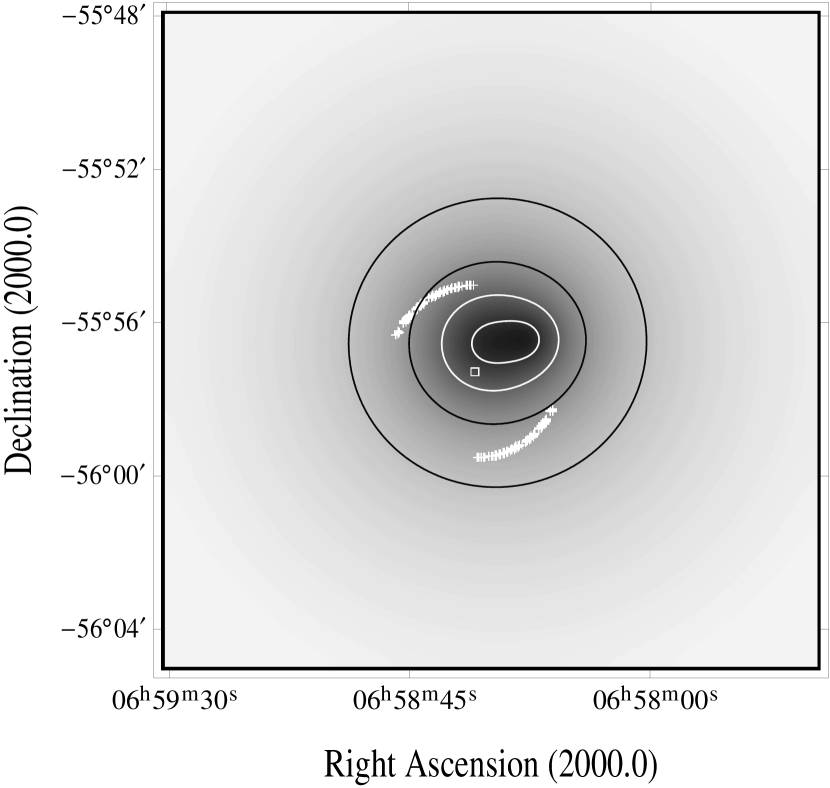
Figure 7: The convolved S-Z surface brightness predicted with the X-ray model described in §4.1. Superimposed are the northern and southern arcs of the reference beams (crosses) and the position of the main beam (open square).

Figure 8: Transmission spectra of the two optical trains defining the wavelength ranges of the two channels at 1 mm ($\sim$ 8.5 $cm^{-1}$) and at 2 mm ($\sim$ 5 $cm^{-1}$).

References

- Aghanim et al. (1997) Aghanim N., De Luca A., Bouchet F.R., Gispert R. and Puget J.L., 1997, astro-ph/9705092
- Andreani (1994) Andreani P. 1994, ApJ 428, 447
- Andreani et al. (1996a) Andreani P., Dall’Oglio G., L. Martinis, Böhringer H. Shaver P., Lemke R., Pizzo L., Nyman L.-Å. Booth R., Whyborn N 1996a, in Proceedings of the XVIth Moriond Astrophysics Meeting, les Arcs, France, March 1996, eds Bouchet F.R., Gispert R., Guiderdoni B., p. 371
- Andreani et al. (1996b) Andreani P. Pizzo L. Dall’Oglio G., Whyborn N., Böhringer H. Shaver P., Lemke R., Otàrola A., Nyman L.-Å. Booth R. 1996b, ApJ 459, L49
- Andreani & Franceschini (1996) Andreani P. & Franceschini A. 1996c,MNRAS 283, 85
- Barrow et al. (1984) Barrow J.D., Bhavsar S.P., & Sonoda D.H. 1984, MNRAS 210, 19p
- Birkinshaw & Gull (1984) Birkinshaw & Gull S.F. 1984, MNRAS 206, 359
- Birkinshaw (1991) Birkinshaw M.: 1991, in Physical Cosmology, ed. A.Blanchard et al. (Gif-sur-Yvette: Editions Frontiéres), p. 177
- Birkinshaw (1997) Birkinshaw M.: 1997, Physics Reports, in press
- Birkinshaw & Hughes (1994) Birkinshaw, M. & Hughes, J. P. 1994, ApJ , 420, 33
- Birkinshaw, Hughes & Arnaud (1991) Birkinshaw, M., Hughes, J. P., & Arnaud, K. A. 1991, ApJ , 379, 466
- Bregman & Cox (1997) Bregman J.N., Cox. C.V., 1997, astro-ph/9712171
- Böhringer et al. (1994) Böhringer H., 1994, in Studying the Universe with Clusters of Galaxies, H. Böhringer and S.C. Schindler (eds.), Proceedings of an astrophysical workshop at Schloß Ringberg, Oct. 10-15, 1993, MPE Report No. 256, p. 93 - 105
- Böhringer & Tanaka (1997) Böhringer H., Tanaka Y, 1997, in preparation
- Cavaliere et al. (1979) Cavaliere, A., Danese, L. & DeZotti, G. 1979, A&A, 75, 322
- Cavaliere & Fusco-Femiano (1976) Cavaliere A. & Fusco-Femiano R. 1976, A&A, 49 137
- Carlstrom et al. (1996) Carlstrom J.E., Joy M., Grego L. 1996, ApJ , 456 L75
- Cen (1998) Cen R., 1998, ApJ 498, L99
- Challinor & Lasenby (1998) Challinor A., Lasenby A. 1998, ApJ 499, 1
- Franceschini et al. (1991) Franceschini A. et al. 1991, A&AS 89, 285-310
- Gautier et al. (1992) Gautier T.N., Boulanger F., Perault M., Puget J.L., 1992, AJ 103, 1313
- Grainge et al. (1993) Grainge K. et al.: 1993, MNRAS 265, L57
- Guzzo et al. (1995) Guzzo, L., Böhringer, H., Briel, U.G., Chincarini, G., Collins, C.A., DeGrandi, S., Ebeling, H., Edge, A.C., Neumann, D.M., Schindler, S., Schuecker, P., Seitter, W.C., Shaver, P., Vettolani, G., Cruddace, R., Fabian, A.C., Gursky, H., Gruber, R., Hartner, G., MacGillivray, H.T., Maccagni, D., Pierre, M., Romer, K., Voges, W., Wallin, J., Wolter, A., Zamorani, G., 1995, in Wide-Field Spectroscopy and the Distant Universe, S.J. Maddox and A. Aragón-Salamanca (eds.), World Scientific, Singapore.
- Haehnelt & Tegmark (1996) Haehnelt, M. G. & Tegmark, M. 1996, MNRAS , 279, 545
- Herbig et al. (1995) Herbig, T., Lawrence, C. R., Readhead, A. C. S., & Gulkis, S. 1995, ApJ , 449, L5
- Holzapfel et al. (1997) Holzapfel, W. L., Ade, P. A. R., Church, S. E., Mauskopf, P. D., Rephaeli, Y., Wilbanks, T. M. & Lange, A. E. 1997, ApJ 480, 449
- Inagaki Suginohara & Suto (1995) Inagaki Y., Suginohara T., Suto Y., 1995, PSAJ 47, 411
- Jones et al. (1993) Jones, M. et al. 1993, Nature, 365, 320
- Klein et al. (1991) Klein U., Rephaeli Y., Schlickeiser R., Wielebinski R., 1991, A&A 244, 43
- Moshir et al. (1989) Moshir M. et al., 1989, Explanatory Supplement to the IRAS Faint Source Survey, Pasadena:JPL
- Myers et al. (1997) Myers, S. T., Baker, J. E., Readhead, A. C. S., Leitch E.M. & Herbig, T. 1997 ApJ 485, 1
- (32) Neumann D., Böhringer H., 1997, MNRAS 289, 123
- Pizzo et al. (1995) Pizzo L., Andreani P., Dall’Oglio G., Lemke R., Otàrola A., Whyborn N., 1995, Exp. Astron. 6, 249
- Press & Teukolsky (1990) Press W.H. & Teukolsky S.A., 1990, Computer in Physics 4, 669
- (35) Rephaeli, Y. 1995a, Ann. Rev. Astr. Ap. , 33, 541
- (36) Rephaeli, Y. 1995b, ApJ , 445, 33
- Roettiger Stone & Mushotzky (1997) Roettiger K., Stone J.M., Mushotzky R.F., 1997, ApJ 482, 588
- Stickel et al. (1997) Stickel M., Lemke D., Mattila K., Haikala L.K., Haas M., 1997 A&A in press
- Sunyaev & Zel’dovich (1972) Sunyaev, R. A. & Zeldovich Ya.B. 1972, Comm.Astr.Spa.Phys. 4, 173
- Sunyaev & Zel’dovich (1981) Sunyaev, R.A. & Zeldovich Ya.B. 1981, Astrop.Spa.Sci.Rev. 1, 11
- Sunyaev & Zel’dovich (1980) Sunyaev, R. A. & Zel’dovich, Ya. B. 1980, MNRAS , 190, 413
- Tucker (1995) Tucker W. H., Tananbaum, H., Remillard, R.A., 1995, ApJ 444, 532
- Tucker et al. (1998) Tucker, W., Blanco, P., Rappoport, S., David, L. Fabricant, D., Falco, E.E., Forman, W., Dressler, A., Ramella, M., 1998, ApJ, 496, L5.
- Ulich (1981) Ulich B.L. 1981, AJ 86 1619
- Ulich (1984) Ulich B.L. 1984, Icarus 60, 590
- Wilbanks et al. (1994) Wilbanks, T. M., Ade, P. A. R., Fischer, M. L., Holzapfel, W. L., & Lange, A. E. 1994, ApJ, 427, L75
- Wright (1979) Wright E.L. 1979, ApJ 232, 348
- Zel’dovich & Sunyaev (1968) Zel’dovich, Ya. B. & Sunyaev, R. A. 1968, Ap&SS, 4, 301