THE PHYSICS OF ACCRETION DISKS WITH MAGNETIC FLARES

, Ph. D.

The University of Arizona, 1998

Director: Fulvio Melia

Rapid progress in multi-wavelength observations of Seyfert Galaxies in recent years is providing evidence that X-ray emission in these objects may be produced by magnetic flares occurring above a cold accretion disk. Here we attempt to develop a physically consistent model of accretion disks producing radiation via magnetic flares as well as the optically thick intrinsic disk emission, and apply this model to observations of Active Galactic Nuclei (AGN) and Galactic Black Hole Candidates (GBHCs). The following issues are considered: (1) the pressure equilibrium in the flare region, (2) the reflection and reprocessing of the X-radiation from flares in the underlying disk, (3) the spectra of GBHCs in the context of the model, (4) and the generation of the flares by the disk – the energy budget of the corona.

Our results show that:

(1) The temperature of the disk atmosphere near active magnetic flares in AGN is in the range $1-3\times 10^{5}$ Kelvin, and that the material is relatively non-ionized. This temperature is in a good agreement with the observed rollover energy in the Big Blue Bump (BBB) of Seyfert 1 Galaxies. We thus suggest that the BBB is simply the X-rays from magnetic flares reprocessed into the X-ray skin of the accretion disk.

(2) We suggest an explanation for the recently discovered X-ray Baldwin effect and the controversy over the existence of BBBs in quasars more luminous than typical Seyferts.

(3) Due to an ionization instability and much higher X-ray incident flux, we found that the X-ray skin in GBHCs is nearly completely ionized. Using an approximate model to describe this effect, we calculated the reflected/reprocessed spectrum and the resulting corona spectrum simultaneously. We found that the spectrum of GBHCs in their hard state may be explained with this model, with basically the same parameters for magnetic flares as in the AGN case.

(4) The magnetic energy transport is shown to be large enough to account for the observed amount of X-rays from Seyferts and GBHCs. We predict that X-ray spectra are hard for accretion rates below the gas-to-radiation transition, and that they are softer above this transition.

(5) We collected our results into a diagram that shows how the observational appearance of accreting black holes changes with the accretion rate and the mass of the hole, and compared it with observations of AGN and GBHCs.

Our conclusion is that the agreement between theory and observations is very encouraging and we suggest that the physics of magnetic flares is the physics that should be added to the standard accretion disk theory in order to produce a more realistic description of accretion flows with large angular momentum.

STATEMENT BY AUTHOR

This thesis has been submitted in partial fulfillment of requirements for an advanced degree at The University of Arizona and is deposited in the University Library to be made available to borrowers under rules of the Library.

Brief quotations from this thesis are allowable without special permission, provided than accurate acknowledgment of source is made. Requests for permission for extended quotation from or reproduction of this manuscript in whole or in part may be granted by the head of the major department or the Dean of the Graduate College when in his or her judgment the proposed use of the material is in the interests of scholarship. In all other instances, however, permission must be obtained from the author.

SIGNED:  

ACKNOWLEDGEMENTS

I thank my graduate adviser, Prof. Melia, for years of support and guidance. I feel indebted to Dr. Edward E. Fenimore for support, advising and teaching basics of science ethics while in Los Alamos National Lab (I can say “I want to be Ed Fenimore when I grow up”). The faculty and fellow students of the Moscow Institute of Engineer Physics are thanked most sincerely, since this is where I was first introduced to theoretical Physics and where my mind often returns for a source of motivation and high standards of work. And, of course, numerous faculty members, stuff and students of the Department of Physics, the University of Arizona, are being thanked for providing me with a friendly and productive work environment.

I am also very grateful to my parents for making me who I am and for their understanding when I first left my home town to study Physics, and eventually the country to be a physicist. Finally, my wife, Elena, has been a constant source of happiness and support for me. I thank her for putting up with all the late nights, working weekends, conferences, and for delivering our daughter, Sonia, few hours after my Ph.D. defense.

TABLE OF CONTENTS

toc

Chapter 1 Introduction

1.1 Existing Theories of Accretion Disks

Accretion Disks are among the most luminous and ubiquitous sources in Astrophysics, and they have drawn a good deal of attention from the observing and theoretical communities since the first complete theory of such disks was formulated by Shakura & Sunyaev (1973). The disks are expected to form whenever an interstellar material or wind from nearby stars is captured by the gravitational attraction of the central object (a star or a black hole), but may not accrete via radial in-fall because of the excess angular momentum. From this brief description, it is evident that this situation is met in a variety of astrophysical systems.

In addition, accretion disks in Active Galactic Nuclei (AGN) and Galactic Black Hole Candidates are believed to harbor a black hole – a very controversial object, a complete understanding of which should provide the modern physics with new horizons. In order to put observational constraints on the black hole physics, we need a thorough understanding of the physics and spectra of ADs. Yet a convincing accretion disk theory, capable of explaining spectra from many types of objects where these disks are expected to form, is still being searched for. The goal of this work is to expand our theoretical understanding of one of the several existing theories, and to motivate future work on that model. Our first task is then to briefly describe the existing theories of accretion disks, and to point out any difficulties or unresolved questions.

1.1.1 Shakura-Sunyaev (Standard) Theory

Shakura and Sunyaev (1973), and several other workers (e.g., Novikov & Thorne 1973), built an accretion disk theory in which the viscosity of the disk material was parameterized through a parameter $\alpha$ – the so-called viscosity parameter. These authors employed equations for angular momentum conservation, vertical pressure balance and energy balance between viscous heating and vertical radiation transport. The radiation field was assumed to be local blackbody emission. This theory is still the most widely cited and successful out of accretion disk theories, since it provides a fair description of AD observations (e.g., Frank et al. 1992, §5.7), especially when the outer part of the disk is concerned.

However, it is clear that in the innermost accretion disk region, i.e., within $\sim$ few tens $R_{g}$ ($R_{g}$ is the gravitational radius, i.e., $R_{g}=2GM/c^{2}$, and $M$ is the black hole mass), the model fails, since observed spectra deviate substantially from simple blackbody model of Shakura and Sunyaev (1973). Spectrum of almost any accretion disk system contains a power-law component up to hard X-rays/soft $\gamma$-rays. In some objects (see Chapter 4), the hard X-rays dominate the overall energy output. This fact is impossible to reconcile with the standard theory. Furthermore, the model is viscously and thermally unstable for high accretion rates, when the disk pressure is dominated by the radiation pressure.

An extensive theoretical effort went into search for a better theory, with inconclusive results so far. A simplest modification to the theory is to assume that the viscosity law in the disk is different from the one prescribed by the standard theory. For some viscosity laws this eliminates the disk instability (e.g., Lightman & Eardley 1974). This does not help to resolve the issue of the spectrum, however, and so does not constitute a satisfactory model.

1.1.2 Two Temperature Model

The two-temperature disk model was suggested by Shapiro, Lightman & Eardley (1976) to explain Cyg X-1, a Galactic Black Hole Candidate (GBHC) that exhibited hard X-ray spectrum up to hundreds of keV, rather than multi-temperature disk blackbody spectrum. The model is based on the assumptions that electrons and protons are coupled by Coulomb collisions only. In this case it turns out to be possible for protons to be much hotter than the electrons. The proton thermal pressure dominates over the radiation pressure in this model, and the model is viscously stable. Electron temperature turns out to be such that the model may explain the hard X-ray spectrum. For a recent work on the model, see Misra & Melia (1996), and further references there.

However, the model is thermally unstable (for a discussion of the disk instabilities, see Frank et al. 1992, Chapter 5). Furthermore, there are serious reasons to doubt the plausibility of the assumption of Coulomb interactions being the only way through which electrons receive heat (see §1.1.3 below). Finally, the model cannot be reconciled with the fact that the cold disk stretches all the way down to the last stable orbit in AGNs (§1.2).

1.1.3 Advection Dominated Accretion Flows

Advection Dominated Accretion Flows (ADAF) have recently received a considerable attention (e.g., Narayan & Yi 1994, 1995, Abramowicz et al. 1995a). The model assumes the same Coulomb-only connection between electrons and much hotter protons. The latter are nearly virialized, and the proton pressure is large enough to make the accretion disk geometrically thick (i.e., the disk scale height $H$ is of the order of the local radius $R$). The gas is optically thin, and the electron temperature is assumed to be much smaller than the proton temperature, and so the disk radiates not as effectively as the optically thick Shakura-Sunyaev disk. Further, since radial velocity $v_{R}$ scales as $v_{R}\sim\alpha c_{s}H/R\propto\alpha(H/R)^{2}$, the advective energy flux is much greater than it is in the standard theory. Due to these reasons, the advection of energy into the black hole, rather than local release of energy through radiation becomes possible. The model predicts that the radiative efficiency of the accretion process is very low, in contrast to usual value $\sim 0.1$ for the standard accretion disk theory.

The model has been applied to a number of accretion disk systems and observations, and has been claimed to be successful in many of these cases. However, we will argue that, at least in some cases, the explanations offered are hardly predictive, and should rather be considered to prove that the model contains enough parameters to reproduce the main features of observed spectra, if these parameters are varied in a way that fits the data.

It is of particular concern to us that the model neglects any electron heating mechanism but Coulomb collisions (see Bisnovatiy-Kogan & Lovelace 1997 for a critique of this assumption; also Begelman & Chiueh 1988). The magnetic fields are assumed to be important only for synchrotron emission, which is hardly justified, since magnetic fields close to the equipartition value are extremely buoyant (see Chapters 2 and 6). When these fields rise out of the disk into a lower density corona environment, they may reconnect. If the electrons are to stay much cooler than the protons, all the reconnection energy must be channeled to and be retained by protons, which (to my knowledge) has never been convincingly demonstrated to be the case. This reconnection process should lead to additional deposition of energy into the electrons and thus an emission not taken into account in the ADAF model. For these reasons, we believe that internal consistency of this model is yet to be proven.

In addition, in the case of AGNs, where observations offer an invaluable tool – the fluorescent iron line – with which to determine the structure of the disk in the innermost region, the ADAF model is clearly ruled out since the cold disk must exist as close as $3R_{g}$ from the black hole (§1.2). One may argue that disks in GBHCs do not show such a line, and thus the material there is hot in the inner disk region. However, in Chapter 4 we will show that the iron line would not even be produced if the same physical model, developed for the AGN case, is applied to GBHCs. Summarizing, we see no reason to believe that ADAF are either internally self-consistent as a theory, or exist in Nature, except possibly for very low accretion rates ($\lower 2.15277pt\hbox{$\;\buildrel<\over{\sim}\;$}10^{-4}$ of the Eddington value) in some cases.

1.1.4 Accretion Disks with Coronae

Liang & Price (1977) were the first to suggest that the X-rays coming from Cyg X-1, and other accreting blackholes, are produced in a hot tenuous corona above the cold disk. Their model was motivated by observations of hot corona on the Sun and stars in general. The model, in its present day version – the two-phase patchy corona-disk model – is consistent with observations of Seyfert Galaxies. This model is the subject of our study here, and is considered in detail in the next section.

1.2 Observational Motivation and Fundamentals of the two-phase model

Here we present a short summary of the current state of the two-phase patchy corona-disk model. By this we mean the purely “empirical” two-phase model, i.e., the model suggested by observations of Seyfert Galaxies with no reference to magnetic flares whatsoever. (We call the model “empirical” because, with the exception of Haardt et al. (1994), one typically makes many key physical assumptions with no hint of a physical proof – see §1.2.1. It is only when one starts to discuss the physics of the model that the necessity of magnetic fields becomes evident). The purpose of our discussion here is to let the reader, possibly not very familiar with current models of the X-ray observations of Seyferts, to see that the two-phase model is an excellent explanation of the observations and that it is actually hard to see how a different physical model can explain the observational facts. Many arguments mentioned in this section, as well as further references to the literature, can be found in excellent reviews by Haardt (1996), Maraschi & Haardt (1996), Svensson (1996a,b).

Observations of Radio Quiet Seyfert Galaxies show that most of the radiation power is contained in the two distinct components: the high energy part – a power-law with an exponential rollover at around several hundred keV, and the broad bump between optical to soft X-ray energies, frequently referred as the Big Blue Bump (BBB, e.g., Walter & Fink 1993). In most cases the power emitted in X-rays is comparable but not larger than that in the optical-soft X-ray band. This fact alone means that there has to be two phases in the inner part of the accretion disk: the hot phase that emits X-rays and the cold one that produces UVs, since it is well known that most of the accretion power is liberated at the smallest radii, where the gravitational energy per particle is the largest. If the inner accretion disk was composed of just one hot phase, as several accretion disk theories predict (e.g., Shapiro, Lightman & Eardley 1976, Narayan & Yi 1994, 1995), then the UV component could never be dominant because of its origin in the outer region of the disk.

There are numerous confirmations to this simple energy argument. Haardt & Maraschi (1991, 1993) identified the hot phase with a corona on the top of the cold phase – the accretion disk, thought to be reasonably well described by the standard accretion disk theory (e.g., Shakura & Sunyaev 1973). They showed that if most of the energy is dissipated in the hot corona rather than in the cold disk, then the resulting spectrum naturally explains many of the observed features in these sources. In particular, they argued that since the emission process is roughly isotropic, about half of the coronal X-ray radiation is directed towards the cold disk, where it gets absorbed and re-emitted as UV radiation, which then re-enters the corona and contributes to the cooling of the electrons. Thus, the coronal gas cooling rate becomes proportional to its heating rate. It is this proportionality of heating and cooling that makes the inverse Compton up-scattering of the UV radiation in the corona to produce an almost universal X-ray spectral index. This ability to reproduce the observed narrow range in the X-ray spectral index (e.g., according to Nandra & Pounds 1994, $\alpha\simeq 1.95\pm 0.15$ for a sample of Seyfert Galaxies) is one of the strongest points of the model.

Further, the hardening of the spectrum above about 10 keV (Nandra & Pounds 1994) was understood as due to the broad hump centered at $\sim$ 50 keV (e.g., Zdziarski et al 1995). The shape of the hump is well described by the Compton reflection of the hard X-rays in the cold disk (e.g., White, Lightman & Zdziarski 1988, Pounds et al. 1990). The inferred solid angle of the cold phase as seen from the corona is a large fraction of $2\pi$, which points to a geometry of the X-ray source placed above a plane of cold material. Moreover, the corona plus cold disk geometry is also supported by the fact that reprocessing of the X-rays into the UV range in the cold disk can naturally account for the observation of correlated variability of the UV and X-rays (e.g., Clavel et al. 1992). Additional and significant support for this geometry comes from observations of the broad iron K$\alpha$ lines, since the shape of these lines cannot be easily understood without invoking a cold accretion disk persisting as close as $\sim 3$ gravitational radii to the black hole (e.g., Reynolds & Begelman 1997 and references there).

However, observationally the X-ray luminosity, $L_{\rm x}$, can be a few times smaller than the UV luminosity $L_{\rm UV}$. This is inconsistent with the two-phase disk- full corona model, because the latter predicts about the same luminosity in both X-rays and UV (due to the fact that all the UV radiation arises as a consequence of reprocessing of the hard X-ray flux, which is about equal in the upward and downward directions). To overcome this apparent difficulty, Haardt, Maraschi & Ghisellini (1994) introduced a patchy disk-corona model, which assumes that the X-ray emitting region consists of separate ‘active regions’(AR) independent of each other. In this case, a portion of the reprocessed as well as intrinsic radiation from the cold disk escapes to the observer directly, rather than entering ARs, thus allowing for a greater ratio of $L_{\rm UV}/L_{\rm x}$. This model is commonly called the two-phase patchy corona-accretion disk model.

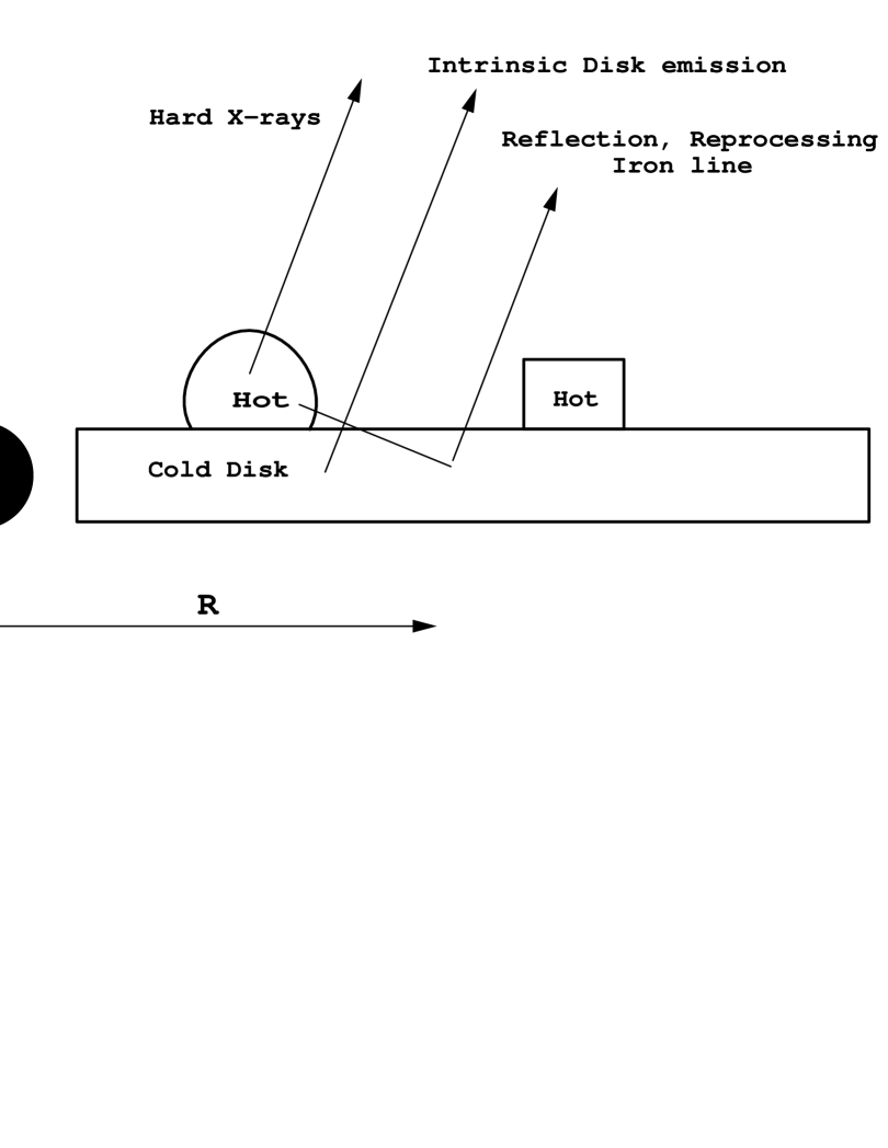
Figure 1.1: The geometry of the two-phase patchy corona-disk model. The accretion disk is assumed to be cold up to the last stable orbit, and X-rays originate in hot active regions above the disk. X-ray flux from an AR is much greater than the disk intrinsic flux. Reflection of X-rays off the “cold” disk accounts for the Iron K$\alpha$ line and correlated variability of UV and X-rays.

Recently, Stern et al. (1995) and Poutanen & Svensson (1996) carried out state of the art calculations of the radiative transport of the anisotropic polarized radiation, for a range of AR geometries. They showed that this type of model indeed reproduces the observed X-ray spectral slopes, the compactness, and the high-energy cutoff if the geometry of the source is hemisphere-like rather than a slab. The cutoff value is explained as being due to pair equilibria in a hot mildly relativistic plasma (e.g., Fabian 1994) and requires a high compactness parameter (for definition see below). The model has very few parameters, namely, the compactness parameter and the temperature of the intrinsic/reprocessed radiation from the cold disk.

To summarize this discussion, we show the geometry of the inner accretion disk learned from the spectral modelling in Figure (1.1). Note that the usual assumption that all the power is dissipated in the active regions is physically equivalent to saying that the X-ray flux from the AR substantially exceeds the disk intrinsic flux, which has to be true only in the immediate vicinity of the AR. It is then not necessary to transfer most of the disk power to the corona to reproduce the correct X-ray spectra.

1.2.1 Deficiencies of the model

Despite the considerable (and unmatched by any other theory) success in the interpretation of observations of Seyfert Galaxies, the two-phase patchy corona-accretion disk model is often criticized for its lack of a self-consistent calculation of the physics of the active regions and the magnetic flux tubes that create these regions. Basically, it is fair to say that there is no complete and detailed physical account of how the accretion disk and magnetic flares can work together. Indeed, even though a very important first step to provide some base for the model was done by Haardt, Maraschi & Ghisellini (1994), who showed that an individual magnetic flare can sustain a high enough energy release rate, several very crucial questions were not addressed by the model. In particular, it has never been questioned whether the two-phase model can provide enough overall power in X-rays to explain the observations (i.e., enough active regions at any given time), since the spectral fitting applied to Seyfert Galaxies addressed the shape of the spectrum, but not its normalization. In addition, the high energy cutoff of the spectrum is controlled by the Thomson optical depth of the AR, and the model assumes that it is given by the pair creation and annihilation equilibrium. However, this approach avoids consideration of the pressure balance in the X-ray source, that is, the confinement of the source. Essentially, one puts particles inside of an artificial rigid box, which is highly unsatisfying physically (see Chapter 3). Furthermore, due to the fact that covering fraction of the patchy corona may well be tiny (see §2.5.5), the local X-ray flux incident on the surface of the cold disk can be larger by several orders of magnitude than that assumed by all existent X-ray reflection calculations. This implies that the static X-ray reflection calculations typically performed are in question when one considers magnetic flares, and thus the whole spectral calculation is in question as well.

1.3 Philosophy and Main Goals of This Work

As we already discussed, the two-phase patchy corona-disk model enjoys a considerably success in explaining observations of X-ray bright Seyfert Galaxies spectra, and yet it is not a fully self-consistent physical model. The model does not include so far, even though it urgently needs it, some input of the physics from “another” research field – the field of magnetic flares. Similarly, the information gained due to the spectral studies of the two-phase model has not been appreciated or used by magnetic flare workers. As a matter of fact, the spectroscopic modelling of X-rays from Seyfert Galaxies and the theoretical studies of magnetic flares seem to exist independently and unaware of each other. It is obvious to us that this strange situation must be changed as soon as possible, if we are to really advance our understanding of physical processes in accretion disks around black holes in AGNs and GBHCs. This is the goal of the present work.

We will select problems that are of most interest for current observations of accretion disks in AGN and GBHCs. We believe it should be our primary task to show that the model provides an appealing framework for many observed phenomena, and that it is time for a strong theoretical effort to understand magnetic flares in accretion disks. In line with this plan, we will keep discussion of the actual magnetic energy release mechanism to a minimum. One reason for this is that we feel it is quite model dependent, since the physics of magnetic reconnection is not understood quantitatively. Second, under certain circumstances, the resulting spectrum does not depend sensitively on the details of the particle energising mechanism. This consideration (§2.5.6) enables us to make some qualitative and quantitative predictions that are needed in order to compare the theory and observations.

Most of our discussion will be devoted to the connection between magnetic flares and the accretion disk, since this connection is most essential when issues of the global spectral behavior of accretion disks are concerned. Further, we should be honest to note that neither we nor anybody else for that matter can build the theory of magnetic flares in accretion disks starting from first principles at this time. It is advisable and promising to start with observations, and attempt to understand whether we can see what characteristics the flares must posses in order to explain these observations. Then, once we have those constraints, we will try to develop the theory taking those constraints into account, which will lead to testable theoretical predictions. Since we plan to use constraints from observations of such diverse objects as AGN (blackhole mass of $\sim 10^{8}$ or more Solar masses ${\,M_{\odot}}$) and GBHCs (blackhole mass of $\sim 10{\,M_{\odot}}$), our hope is that this will allow us to find any strong and weak points of the theory.

Chapter 2 Magnetic Flares in Accretion Disks: Preliminaries

2.1 Basics of Magnetic Flare Physics

One of the important facts learned from observations of turbulent, differentially rotating fluids is that they generate magnetic fields (Parker 1979, Priest 1982, Tajima & Shibata 1997). Another surprising observation is that these fields are not distributed uniformly in the fluid, but tend to concentrate into strong magnetic flux tubes, with magnetic pressure of the order of the ambient gas pressure. For example, Solar observations show that as much as $90$% of the overall Solar surface magnetic energy is in the form of magnetic flux tubes (see references in Parker 1979, §10.1). This concentration of the field to the flux tubes is truly amazing, since the volume average of the magnetic pressure outside the flux tubes is smaller than the gas pressure (which is about the maximum that magnetic pressure in the flux tubes can attain) by a factor probably as large as $\sim 10^{6}$!

The next well understood (qualitatively, if not quite quantitatively yet) feature of the magnetic flux tubes in astrophysical plasmas is that these tubes are buoyant with respect to the fluid that contains less magnetic field (Parker 1955). The magnetic buoyancy is somewhat similar to convection. Convection is caused by the fact that a parcel of gas hotter than its surroundings is less dense due to the pressure equilibrium between the parcel of the gas and the ambient gas. This parcel of gas is then lighter and is buoyant with respect to the rest of the fluid. Similarly, a magnetic field provides pressure, but not the mass density, thus making the gas possessing the field to be buoyant. In principle one could construct equilibria such that magnetic buoyancy is balanced by other forces, e.g., magnetic tension, but these situations are often found unstable, so that magnetic buoyancy is always important, as soon as strong magnetic fields exist (Parker 1979, chapter 13).

It is thought that the phenomenon of buoyantly rising magnetic flux tubes explains appearance of strong and concentrated magnetic fields above the Solar surface, and eventually, magnetic flares that are observed (e.g., Tsuneta 1996, Tajima & Shibata 1997, §3.3). Figure (2.1) shows an X-ray image of the Sun obtained with the Yohkoh Solar mission. Several active magnetic flares are clearly seen. Note the localized and turbulent nature of the X-ray emitting corona, which consists of many magnetic loops. Magnetic flares may be defined as a rapid transfer of magnetic energy to the gas trapped inside the flux tubes, leading to radiation with photon energies up to hard X-rays. To understand why the energy release happens above the Solar or accretion disk surface, and not where the fields were originally produced, one should notice that Solar or accretion disk plasmas are ideal in the MHD sense to a large degree, and thus the magnetic flux (energy) is conserved, that is, it cannot be transferred to particles. Above the disk, however, the gas density is very low, and there is a possibility for the reconnection process (breakdown of ideal MHD). Both theory and observations of reconnection process (see, e.g., Parker 1979, Priest 1982, Tajima & Shibata 1997 §3.3), the reconnection rate is (see Parker 1979, Priest 1982, Tajima & Shibata 1997) proportional to the the Alfvén velocity $V_{\rm A}\equiv B/\sqrt{4\pi\rho}$, where $B$ is magnetic field intensity and $\rho$ is the gas density. Therefore, inside the flux tubes above the disk where the gas density is low the reconnection can happen at a much higher rate than in the mid-plane.

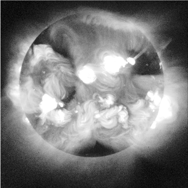
Figure 2.1: This is an X-ray image of the sun taken at 07:33 UT on 12 November 1991 and is described in the article ”The Yohkoh Mission for High- Energy Solar Physics”, by L. Acton, et. al., Science vol. 258 , 23 Oct. 1992 pp. 618-625. Picture brightness scales as the logarithm of intensity. A thin aluminum filter restricted the instrument bandpass to the 3 to 40 Angstrom wavelength interval ($\sim$ 0.3 – 4 keV). The hot ionized gases in the solar atmosphere which emit in this interval trace the solar magnetic fields extending up into the corona.

2.2 Magnetic Fields and Flares in Accretion Disks

Since it is well established that magnetic flares do occur on the Sun, it is useful to draw a parallel between Solar and the accretion disk physical conditions. We shall discuss some of the differences in radiation mechanisms in Solar and accretion disk flares in §2.5.6, but for now it is interesting to just question why we would expect substantial magnetic field effects in accretion disks at all. It is believed that plasma differential motions generate magnetic fields (e.g., Tajima & Shibata 1997, §3.1). A useful number is then the ratio of the gas differential velocity $v_{d}$ to the sound speed $c_{s}$. To estimate that, one can take the differential velocity to be the change in the gas rotational velocity between points separated by the length scale typical of the region where the fields are produced. In the case of the Sun, we should take 0.1 of the Solar radius, since this is probably the depth of the convection zone. With that we obtained $v_{d}/c_{s}\sim 0.01$. In the accretion disk case, the appropriate typical dimension is the disk scale height (see Galeev et al. 1979). The standard accretion disk theory then yields $v_{d}/c_{s}\sim 1$. Accordingly, we should expect that accretion disks are much more magnetically active astrophysical objects than stars.

Galeev, Rosner & Vaiana (1979) were the first to show that magnetic flares are likely to occur on the surface of an accretion disk, since the internal dissipative processes are ineffective in limiting the growth of magnetic field fluctuations. As a consequence of magnetic buoyancy, magnetic flux should be expelled from the disk into a corona, consisting of many magnetic loops, where the energy is stored. Galeev et al. (1979) also speculated that just as in the Solar case, the magnetically confined, loop-like structures produce the bulk of the X-ray luminosity. The X-rays were assumed to be created by Compton upscattering of the intrinsic disk emission or by bremsstrahlung.

Since then, several workers have elaborated on this subject (e.g., Kuperus & Ionson 1985; Burm 1986; Burm & Kuperus 1988; Stepinski 1991; de Vries & Kuijpers 1992; Volwerk, van Oss & Kuijpers 1993; van Oss, van Oord & Kuperus 1993, Field & Rogers 1993). Unfortunately, all of these models were very much more complicated than simpler plasma models, e.g., Poutanen & Svensson (1996), that take into account the detailed interaction of particles and radiation but leave out the question of how the plasma is confined and energy is supplied. Consequently, there were no agreement even among the accretion disk magnetic flare theorists as to what spectrum will result from magnetic flares. Thus, although the magnetic flares above the cold accretion disk were a recognized possibility for the X-ray emission from accretion disk, the model lacked predictive power and was not popular among the observing community.

An important step forward was done by Haardt, Maraschi & Ghisellini (1994), who for the first time attempted to connect the physics of magnetic flares with the observational need for localized active regions above the disk. These authors showed that physical conditions for the gas trapped inside a magnetic flare may well be similar to those required by the two-phase patchy corona-disk model. This really brought the magnetic flare model on a new, testable level, since with this work it became clear that due to high compactness parameter (see §2.4) of the plasma in the active regions, the dominant emission mechanism is Comptonization (see Fabian 1994), which always leads to a power-law plus exponential roll-over with X-ray spectral indexes (for this type of geometry) close to those actually observed in Seyfert Galaxies. However, the model was still too vague and had many unresolved questions (e.g., §1.2.1).

2.3 Cold Accretion Disk Structure

The magnetic flares are “slaves” to the underlying accretion disk, they are created and controlled by it. Our first goal then is to introduce some sort of accretion disk model that would be compatible with the well understood accretion process physics (e.g., Frank et al. 1992) and the presence of magnetic flares. In general it is an impossible task, but we may approximate the situation by noting that as long as vertically and time averaged disk quantities are concerned, the magnetic flares are just another energy transport mechanism (in addition to the usual radiation flux). We will find that the volume average magnetic pressure is likely to be rather small compared to the gas pressure in the disk, so we need not worry about magnetic pressure effects. The additional energy transport, on the other hand, should be included in the vertical energy balance equation as an additional cooling. We found the approach of Svensson & Zdziarski (1994; SZ94 hereafter) to be the most practical here. These authors considered a uniform corona above the standard accretion disk, and allowed a fraction $f\leq 1$ of the total local gravitational energy release to be channeled to the magnetic energy transport, and the rest, i.e. $1-f$ to be transported via the usual radiation diffusion energy flux. Since the heating of the disk interior by the incident X-rays is negligible in both static and flaring corona, the disk structure should be adequately described by this formalism. The main results of studies conducted by SZ94 is that such disk plus corona system is depicted by the standard accretion disk theory “corrected” by the factor $1-f$; the accretion disk is cooler (because energy is vented away by the flares) and that the disk may be more stable to viscous and thermal instabilities than the standard disk is for the same $\dot{m}$. $\dot{m}$ here is the dimensionless accretion rate, defined as $\dot{m}=\eta\dot{M}c^{2}/L_{\rm Edd}$, where $\eta=0.06$ is the efficiency of gravitational energy conversion into radiation, $\dot{M}$ is the actual accretion rate in the physical units, and $L_{\rm Edd}$ is the Eddington luminosity. Note that in this definition $\dot{m}=1$ corresponds to the total luminosity equal to $L_{\rm Edd}$, and that our definition of $\dot{m}$ is that of SZ94 times $\eta$.

For our discussions throughout this paper, we will often need typical numbers for the gas mid-plane temperature $T_{d}$, the disk effective temperature $T_{\rm eff}$, ratio of the pressure scale height $H$ to the radius $R$, and the disk intrinsic flux $F_{d}$. We write these quantities below using corresponding equations of SZ94. In writing down the quantities mentioned above, we will choose $R=6R_{g}$ as a typical radius where the flares occur. The gas-dominated solution yields:

$${H\over R}=2.25\times 10^{-3}\left(\alpha M_{8}\right)^{-1/10}\dot{m}^{1/5}\left[\zeta(1-f)\right]^{1/10}$$ (2.1)

$$F_{\rm d}=2.\times 10^{16}\dot{m}(1-f)M_{8}^{-1}{\rm erg\ cm}^{-2}\;{\rm sec}^{-1}$$ (2.2)

$$T_{d}=2.2\times 10^{6}\left(\alpha M_{8}\right)^{-1/5}\dot{m}^{2/5}\left[\zeta(1-f)\right]^{1/5}\;{\rm K}$$ (2.3)

$$T_{\rm eff}=1.4\times 10^{5}\left[\dot{m}(1-f)\right]^{1/4}M_{8}^{-1/4}\;{\rm K}$$ (2.4)

and the “critical” accretion rate, at which the transition from the gas-dominated to the radiation-dominated solution takes place, is $\dot{m}_{\rm cr}$, where

$$\dot{m}_{\rm cr}=2.2\times 10^{-3}\left(\alpha M_{8}\right)^{-1/8}\left[\zeta(1-f)\right]^{-9/8}{\rm,}$$ (2.5)

where $F_{\rm d}$ is the disk intrinsic radiation flux, i.e., the one transported by the usual radiation transport. The parameter $\zeta$ here describes the uncertainty in the radiation flux from the accretion disk in the vertical direction. This uncertainty is caused by the usual approximate averaging of the disk equations in the $z$-direction instead of finding the exact vertical disk structure. Different authors choose $\zeta$ to lie between $2/3$ and $2$ (see SZ94). We will assume that $\zeta=1$, but will keep in mind that certain quantities, most notably $\dot{m}_{\rm cr}$, depend rather sensitively on this poorly determined parameter.

The-radiation-dominated solution gives

$${H\over R}=0.3\dot{m}\,\left(1-f\right)$$ (2.6)

$$T_{d}=2.1\times 10^{5}\left(\alpha M_{8}\right)^{-1/4}\left[\zeta(1-f)\right]^{-1/4}\;{\rm K}$$ (2.7)

$${P_{\rm rad}\over P_{\rm gas}}=2.0\times 10^{5}\left(\alpha M_{8}\right)^{1/4}\,\dot{m}^{2}\left[\zeta(1-f)\right]^{9/4}{\rm.}$$ (2.8)

2.4 Physical Constraints on the Two-Phase Model

As we detailed in §1.2.1, the two-phase patchy corona-disk model does not provide a full description of the physics of the active regions. In particular, the plasma in the ARs should be confined during the active phase, otherwise the energy will be lost to the expansion of the plasma rather than producing the X-rays. Not confined, the source would expand at the sound speed, which may be a fraction of $c$ for these conditions. It is not clear that the spectrum from such an expanding and short lived source can resemble anything studied thus far in the literature. The familiar gravitational confinement, operating in the main part of the accretion disk, does not work here because there is no mechanism for counter balancing a side-way expansion of the plasma. Therefore, since there seems to be no other reasonable possibility for confinement of the AR plasma, it may be argued that a magnetic field is required to provide the bounding pressure. Without a magnetic field, the AR would expand side-ways at least, and form a slab like corona, which was shown to be incompatible with observations of Seyferts by Haardt et al. (1994) and Poutanen & Svensson (1996).

One of the most restrictive and important parameters of the ARs in the two-phase model is the compactness parameter

$$l\equiv F_{\rm x}\sigma_{T}\Delta R/m_{e}c^{3}\,{\rm,}$$ (2.9)

where $F_{\rm x}$ is the radiation energy flux at the top of the AR and $\Delta R$ is its typical size. The compactness parameter is an indication of the total energy content of the magnetic flare, given its size. Note that this definition is for the local compactness, i.e., the one that characterizes the local properties of the plasma, unlike the global compactness $l_{g}\equiv L\sigma_{T}/R^{\prime}m_{e}c^{3}$, where $L$ is the total luminosity of the object and $R^{\prime}$ is the typical size of the region that emits this luminosity. It is the latter that should be compared to the observed compactness rather than the former.

A local compactness much larger than unity is required by current two-phase thermal models of ARs (e.g., Svensson & Poutanen 1996) in order to provide a large enough Thomson optical depth due to electron-positron pairs. However, we note there is no a priori reason why pair production must be important, other than the fact that under some conditions it could explain the observed electron temperature (e.g., Fabian 1994, but see chapter 3). Maciolek-Niedzwiecki, Zdziarski & Coppi (1995) have shown that the annihilation of thermal electron-positron pairs always produces a broad spectrum of the resulting photons, and that it is very hard, if possible at all, to single out this component from the total spectrum on the background of the dominant Comptonized spectrum. Thus, we really cannot tell based on the spectra alone whether pairs are abundant on not in the X-ray producing regions of AGN or GBHCs. In fact, due to spectral constraints on the X-ray reprocessing, we find (Chapters 4 & 5) that the pairs are not likely to be important.

A more stringent constraint on the value of $l$ is the free-free emission from the active region to be negligible (not to destroy the two-phase energy balance). The compactness parameter due to bremsstrahlung emission may be estimated using equation (5.15b) of Rybicki & Lightman (1979):

$$l_{\rm brem}\sim 3.\times 10^{-3}\,\tau_{T}^{2}\,\Theta^{1/2}{\rm,}$$ (2.10)

where $\Theta$ is electron temperature in the units of $m_{e}c^{2}/k_{B}$. For the typical values $\Theta\sim 0.3$, and $\tau_{T}\sim 1$, this requires that $l\gg 10^{-2}$. Finally, since the two-phase model was built under the assumption that the disk intrinsic flux $F_{\rm d}$ is much smaller than the X-ray flux from the active regions, the conditions for the applicability of the model are:

$$F_{\rm x}\gg F_{\rm d}{\rm,}$$ (2.11)

$$l\gg 0.01{\rm.}$$ (2.12)

2.5 Magnetic Flares

2.5.1 Geometry

Figure 2.2: A simple sketch of a magnetic flux tube that broke through the accretion disk surface due to buoyancy. Notice that magnetic flare size cannot be much larger than the accretion disk scale height. The flux tube is “fat”, since there is little bounding pressure above the disk, and the field takes a quasi-potential configuration.

We sketch a typical magnetic flux tube after it has broken up through the surface of the disk in Figure (2.2). The part of the flux tube that is above the accretion disk is the one that produces an active region. On the right of the Figure (2.2) we also show a part of the submerged magnetic flare, which has just started to develop a buoyancy-unstable region. X-ray Solar observations show that magnetic flux tubes can be rather quiet for a relatively long time and then suddenly become active, when they release energy comparable to the total magnetic energy of the tube. It is this release of magnetic energy into radiation that is called a ”magnetic flare”. Note that the geometry of the flares is very similar to what the ARs should look like (compare Figures 1.1 and 2.2).

2.5.2 Compactness of Magnetic Flares

We can estimate the maximum compactness of the magnetic flares by the following considerations (following Haardt et al. 1994). The magnetic field is limited by the equipartition value in the mid-plane of the disk. The size of the AR, $\Delta R$, is of the order of one turbulent cell, which is at most equal the disk scale height $H$ (e.g., Galeev et al. 1979). Let us assume that the field annihilation occurs on a time scale $t_{\rm l}$ equal to the light crossing time $\Delta R/c$ times some number $b\sim 10$. This may be justified by noting that the Alfvén velocity can be close to $c$ for these conditions. We will also assume that the flare occurs at 6 gravitational radii, where the accretion disk energy generation per unit area has a maximum. Using the definition of the local compactness parameter and the results of Svensson & Zdziarski (1994), we obtain:

$$l\lower 2.15277pt\hbox{$\;\buildrel<\over{\sim}\;$}400\,{{\dot{m}}\over\alpha b}\;{\varepsilon_{\rm m}\Delta R\over\varepsilon_{\rm d}H}{\rm,}$$ (2.13)

where $\alpha$ is the standard $\alpha$-parameter of Shakura-Sunyaev viscosity prescription, $\varepsilon_{\rm m}$ is the magnetic energy density in the AR, which must be smaller than the disk mid-plane energy density $\varepsilon_{\rm d}$. Note that the estimate of the compactness parameter (2.13) does not depend on $f$.

For future convenience, we will re-write the above equation as

$$l\simeq 40\,\dot{m}\alpha^{-1}\zeta{\rm,}$$ (2.14)

where we have collected parameters that we cannot accurately calculate at this time in a single quantity $\zeta$, which we expect to be of order of unity. However, due to a very approximate nature of our method to estimate the compactness parameter, we will use this expression as a guide which can tell us how $l$ scales with accretion rate, $\alpha$ and geometry, rather than an exact equation.

2.5.3 The X-ray flux

For the sake of completeness, and for future reference, we should also compare the X-ray flux $F_{\rm x}$ generated by a magnetic flare with $F_{\rm d}$, the flux from the underlying cold disk, as given by equation (2.2). A major assumption of the two-phase patchy corona model is that the X-ray flux greatly exceeds the intrinsic disk flux. If this assumption does not hold, then the spectrum will be steeper than the observed Seyfert spectra. The magnetic flare X-ray flux can be determined from the definition of the compactness parameter (equation 2.9), and equation (2.14). This yields

$$F_{\rm x}=1.\times 10^{17}l\dot{m}^{-1/5}\,M_{8}^{-9/10}\,\alpha^{1/10}(1-f)^{-1/10}{H\over\Delta R}\,{\rm erg\ cm}^{-2}\,{\rm sec}^{-1}{\rm.}$$ (2.15)

One can see that the flux from an active region is very much larger than the disk intrinsic flux, which parenthetically means that the total area covered by magnetic flares should be much smaller than the total inner disk area. This is similar to the Solar X-ray emission, where X-rays come from localized magnetic flares rather than uniformly from the whole disk surface (see Figure 2.1)

2.5.4 Number of Flares and Variability

There are a few other simple but quite valuable estimates that we can make based on the simple energy budget argument. One of these is the average number of active magnetic flares, $N$. To determine it, we will require that $N$ times the luminosity of a single flare equals the overall X-ray luminosity observed from a source. If we assume that almost all X-rays impinging on the cold disk are reprocessed into the UV range, which is a good approximation for AGNs (see Chapters 4 & 5), the X-ray luminosity of the corona-disk system is approximately equal to (Haardt & Maraschi 1991, 1993)

$$L_{\rm x}=(f/2)\,L$$ (2.16)

where $L$ is the bolometric luminosity of the source, and $f$ is the fraction of power transfered to the corona. To find the luminosity $L_{1}$ of a typical flare, we can use the definition of the compactness parameter (equation 2.9), and express $L_{1}$ as $L_{1}\sim\Delta R^{2}F_{\rm x}$. Working through some simple algebra, one obtains

$$N\sim{fL\over 2L_{1}}\sim 10^{3}\left({\dot{m}\over 10^{-3}}\right)\left({R\over 10^{3}\Delta R}\right)l^{-1}(f/2)$$ (2.17)

Here we have scaled $\dot{m}$ and $\Delta R/R$ on values typical for these quantities in Seyfert Galaxies. The often observed short time scale variability of the X-ray continuum from Seyferts by a factor of 2 can be explained by random fluctuations in the number of flares if $N\sim 10$ (e.g., Haardt et al. 1994), which would then suggest that $l\sim 100$. However, one should not forget that flares are controlled by the accretion disk, so, it is possible that the disk modulates the appearance of the flares and thus flares may be not statistically independent events. Thus, the estimate of $N$ based on X-ray variability needs to be put to a serious test before we could constrain $l$ based on it.

Furthermore, the continuum variations happen on time scales from a few hundred to $\sim 10^{5}$ sec (e.g., Done & Fabian 1989), which may be a very short time scale for a massive AGN. For example, the light crossing time of one gravitational radius is $R_{g}/c=10^{3}M_{8}$ sec, where $m_{8}\equiv M/10^{8}{\,M_{\odot}}$. Since any model of X-ray emission from AGNs should be able to reproduce variations on the observed time scales, large scale (i.e., $\sim R_{g}$) emission regions are ruled out. The magnetic flare model is in a better shape here, since the emission regions are very small in size ($H/R\sim 10^{-3}$). To estimate the typical flare life time $t_{l}$, we can write $bH/c\lower 2.15277pt\hbox{$\;\buildrel<\over{\sim}\;$}t_{l}\lower 2.15277pt\hbox{$\;\buildrel<\over{\sim}\;$}2\pi R/v_{\phi}$, where $v_{\phi}$ is the Keplerian velocity. The lowest limit here is equal to $b\geq 10$ light crossing times of the flare region, and the upper limit is equal to one dynamical time scale, i.e., the orbital time scale. This reasoning yields

$$60\;{\rm sec}\;M_{8}\,\lower 2.15277pt\hbox{$\;\buildrel<\over{\sim}\;$}\,t_{l}\,\lower 2.15277pt\hbox{$\;\buildrel<\over{\sim}\;$}2\times 10^{4}\;{\rm sec}\;M_{8}{\rm.}$$ (2.18)

This estimate shows that the typical life time of a flare is in the range of observed variability time scales (see also Galeev et al. 1979 and de Vries & Kuijpers 1992).

2.5.5 Covering Fraction

The other useful number which we may obtain from simple energy budget considerations is the covering fraction of the magnetic flares, i.e., the fractional area $f_{c}$ of the inner accretion disk surface that is covered by active magnetic flares at any time. This fraction may be found by noting that the product of the area covered by magnetic flares $A_{m}$ and the typical X-ray flux should be equal to $L_{\rm x}=(f/2)L$, whereas the product of the disk intrinsic flux $F_{d}$ and the disk area $A_{d}$ should be equal to the disk luminosity $(1-f)L$. Thus,

$$f_{c}\equiv{A_{m}\over A_{d}}\simeq{f\over 2(1-f)}\;{F_{d}\over F_{x}}=10^{-1}l^{-1}\,\dot{m}^{6/5}\,f\,(1-f)^{1/10}\;\left(\alpha M_{8}\right)^{-1/10}\,{\Delta R\over H}{\rm.}$$ (2.19)

Thus, the covering fraction may be quite small for small accretion rates.

2.5.6 Spectra from Magnetic Flares

As a first guess, one would think that it is extremely challenging to accurately compute the spectrum from such a complicated phenomenon as a magnetic flare. The spectrum will depend on the geometry and the unknown distributions of the gas density and temperature in the flaring region. These distributions are dependent on the model assumed for the reconnection mechanism and other factors, and are absolutely impossible to uniquely determine at the present time. In our opinion, this apparent uncertainty in the spectrum is the foremost important reason why the magnetic flares have not been firmly established as a source of X-rays from accretion disks after decades of theoretical studies.

However, the X-ray spectrum from accretion disk magnetic flares should be similar to that of a static active region of the two-phase model of the same size and compactness, as long as the lifetime of the flare exceeds several light-crossing time scales. The repeated inverse Compton upscattering mechanism produces always a featureless X-ray spectrum – a power-law with a quasi exponential roll-over – the form of the intrinsic active region spectrum used to fit the observations of Seyfert Galaxies by Zdziarski et al. (1995). To emphasis how well Comptonized spectra hide the nature of physical processes creating them (and the geometry of the source), we point out that the featurlessness of the spectrum arising from Comptonization was even cited as a principal problem in inferring the shape of the underlying electron distribution via comparison of the spectra produced by thermal and non-thermal Comptonization (Ghisellini, Haardt & Fabian 1993). This is even more so if the observed spectrum consists of many separate contributions from flares with different parameters. Thus, the spectrum of the magnetic flares is adequately described by the two-phase patchy corona model with a correctly chosen geometry and compactness parameter.

The major difference between the Solar magnetic flares and those occurring on the surface of accretion disks is the compactness parameter. For the Solar case, $l\ll 1$, and can be as small as $l\sim 10^{-6}$, as one can check using typical time scales for the energy release and the overall energy content of magnetic flares (e.g., Priest 1982). For the accretion disk magnetic flares, the compactness parameter can be considerably larger, $l\gg 0.01$ (see section §2.5.2). According to §2.4, this implies that bremsstrahlung is far more important than Comptonization for the Solar flare spectra. The other important difference is the Alfvén velocity, which is substantially higher for magnetic flares in disks.

Chapter 3 Pressure Equilibrium and Containment

3.1 Observational Motivation

Haardt et al. (1994) suggested that the active regions (ARs) may be magnetic flares occurring above the accretion disk’s atmosphere and showed that their compactness $l$ may be quite high ($\sim 30$), so that pairs can be created. In principle, it is possible to obtain still larger values for the compactness parameter ($l\sim$ few hundred), thus creating enough pairs to account for the observed $\tau_{T}\simeq 1.0^{+0.4}_{-0.2}$ (Zdziarski et al. 1996), where $\tau_{T}$ is the Thomson optical depth of the AR. This explanation for the observed value of $\tau_{T}\sim 1$ based on the pair equilibrium condition, however, relies on the assumption that the particles are confined to a rigid box, so that no pressure constraints need to be imposed. This is unphysical for a magnetic flare where the particles are free to move along the magnetic field lines. Therefore, as far as the two-phase model without a proper pressure equilibrium condition is concerned, the Thomson optical depth is a parameter, rather than a calculable quantity.

Here we will consider the pressure equilibrium during an intense magnetic flare occurring above the surface of a cold accretion disk. Assuming that the heating source for the plasma trapped in the flaring region is the energy transported by magnetohydrodynamic waves or energetic particles with group velocity close to the speed of light, we show that under certain conditions the pressure equilibrium constrains the Thomson optical depth $\tau_{T}$ of the plasma to be in the range $1-2$. We suggest that this pressure equilibrium may be responsible for the observed value $\tau_{T}\sim 1$ in Seyfert Galaxies. We also consider whether current data can distinguish between the spectrum produced by a single X-ray emitting region with $\tau_{T}\sim 1$ and that formed by many different flares spanning a range of $\tau_{T}$. We find that the available observations do not yet have the required energy resolution to permit such a differentiation. Thus, it is possible that the entire X-ray/$\gamma$-ray spectrum of Seyfert Galaxies is produced by many independent magnetic flares with an optical depth $0.5<\tau_{T}<2$.

3.2 The Connection Between The Energy Supply Mechanism and Pressure Equilibrium

The ‘universal’ X-ray spectral index of Seyfert Galaxies (e.g., Nandra & Pounds 1994) suggests that the emission mechanism is thermal Comptonization with a $y$-parameter close to one (Haardt & Maraschi 1991; Haardt & Maraschi 1993; Fabian 1994). The $y$-parameter is defined here as the average photon fractional energy gain times the average number of scatterings that the photon suffers before it escapes to infinity (e.g., Rybicki & Lightman 1979, Chapter 7). For the emission to be dominated by Comptonization, the compactness parameter needs to be large (e.g., Fabian 1994, and §2.4). Observations of Seyfert Galaxies point to a global compactness parameter $\sim 1-100$ (Svensson 1996 and references cited therein).

For electrons and protons at a single temperature $T_{e}$ and an electron number density $n_{e}$ with the assumption of neutrality, the gas pressure is $2n_{e}kT$. The radiation energy density may be recast in terms of the luminosity $L$ of the source, and therefore its compactness parameter $l$, under the assumption that the typical photon escape time is given by the light crossing time multiplied by $1+\tau_{T}$ (see Rybicki & Lightman 1979). The total pressure is

$$P={m_{e}c^{2}\over\sigma_{T}R}\,\left[2\tau_{T}\,\Theta_{e}+l(1+\tau_{T})/3\,\right]{\rm,}$$ (3.1)

where $\Theta_{e}\equiv kT_{e}/m_{e}c^{2}$ is the dimensionless electron temperature. The Compton $y$-parameter for thermal electrons is $y=4\Theta_{e}\tau_{T}(1+\tau_{T})(1+4\Theta_{e})$ and is of order 1 (e.g., Haardt & Maraschi 1991). Thus, since the dimensionless gas pressure in Equation (3.1) is always smaller than $y$, the radiation pressure dominates over the gas pressure in a one-temperature plasma when $l\gg 1$.

One consequence of this is that the amount of energy escaping from the source even during one light crossing time is larger than the total particle thermal energy. Thus, there must be an agent that energizes the particles to enable them to radiate at this high rate, and the presence of this agent must be dynamically consistent with the state of the system. We foresee two possibilities for the nature of this ‘agent’: (i) the gravitational field, and (ii) an external flow of energy into the system. These two cases are quite distinct physically.

Insofar as the first possibility is concerned, the gravitational potential energy of the plasma (primarily that of the protons) is dissipated as the gas sinks deeper into the well of the black hole. The gravitational field does not provide a pressure, but it does compress the gas. However, this leads to an internal (radiation plus gas) pressure that varies from source to source as the physical conditions change. There does not appear to be a scale that sets $\tau_{T}$ to have a value of $1$. For example, in standard accretion disk theory, the inner radiation pressure-dominated regime has an optical depth that depends on several parameters, such as the accretion rate and the $\alpha$-parameter (Shakura & Sunyaev 1973). The $\alpha$-parameter reflects the rate at which the protons ‘use up’ their potential energy, and so a change in this rate leads to a change in the equilibrium optical depth. It is even less obvious why $\tau_{T}$ should be $\sim 1$ in the gas pressure dominated regimes since there the pressure has no reference to $\tau_{T}$ at all. It seems that when the pressure equilibrium is dictated by the gravitational field (e.g., due to a compression of the X-ray emitting region), the Thomson optical depth should span a range of values depending on the source geometry, the specific parameter values and the particle interactions assumed to operate in the source.

This is not so when the energy is supplied to the X-ray emitting region by an inflow of energy, e.g., via a magnetic field. The principal difference between the two cases is that the dynamic portion of the magnetic field supplies a “ram” pressure that is related in a known way to its energy density. If the magnetic energy flux into the X-ray emitting region is known, this also constrains the inwardly directed momentum flux (the compressional force) into the system. Thus, the compressional force exerted on the active region by the magnetic field is expected to correlate with the source luminosity. What makes this useful in terms of setting the optical depth of the system is that a similar correlation exists between the luminosity and the outwardly directed radiation pressure in the emitting region. But in this case, the pressure also depends on $\tau_{T}$. Assuming a spherical geometry for simplicity, the radiation pressure is $P_{r}\simeq\tau_{T}F_{r}/c$, where $L\approx 4\pi R^{2}F_{r}$ in terms of the source radius $R$ and radiation flux $F_{r}$. Thus, since all the balance equations are to first order linear in $F_{r}$, it is anticipated that the pressure and energy equilibria of the system point to a unique value of $\tau_{T}$. We explore this possibility in the next section.

3.3 Pressure Equilibrium For Externally Fed Sources

Let us first suppose that the X-ray source is a sphere with Thomson optical depth $\tau_{T}$, and that the energy is supplied radially by magnetohydrodynamic waves. The waves carry an energy density $\varepsilon$ and propagate with velocity $v_{A}$. For definitiveness, we assume that these are Alfvén waves, in which case the momentum flux that enters the X-ray source is $(1/2)\,\varepsilon$. The magnetic energy of the Alfvén waves is in equipartition with the oscillating part of the particle energy density, and so we can estimate the gas pressure as being of the same order as the ram pressure of the oscillating part of the magnetic field, i.e. $(1/2)\,\varepsilon$. Finally, we assume that all of the wave energy and momentum are absorbed by the source.

The energy equilibrium for the AR is then given by

$$F_{r}=\varepsilon v_{A}\;,$$ (3.2)

whereas in pressure equilibrium

$$P_{r}\simeq\tau_{T}F_{r}/c\simeq\varepsilon\;.$$ (3.3)

Dividing the latter equation by the former, one obtains for the equilibrium Thomson optical depth:

$$\tau_{T}\simeq{c\over v_{A}}$$ (3.4)

This value does not depend on luminosity, but it does of course depend on the geometry and $v_{A}$. To explain observations, we need $v_{A}\sim c$ (see §3.3.1 below).

Suppose now that the geometry is not perfectly spherically symmetric, and that instead the Alfvén waves can enter the X-ray source through an area $A_{a}$, but the radiation leaves through an area $A_{r}\lower 2.15277pt\hbox{$\;\buildrel>\over{\sim}\;$}A_{a}$, which is plausibly just the total area of the AR. This situation may occur if part of the X-ray source is confined by other than the Alfvén wave ram pressure, e.g., by the underlying (non-dynamic) large-scale magnetic field (see below). In this case, since the energy balance is now $F_{r}A_{r}=\varepsilon v_{A}A_{a}$, the equilibrium $\tau_{T}$ is changed to

$$\tau_{T}\simeq\left({c\over v_{A}}\right)\left({A_{r}\over A_{a}}\right)\;.$$ (3.5)

To understand the scale represented by the bracketed quantities in this equation, let us consider the physical conditions that are likely to be attained during a short-lived and very energetic magnetic flare above the standard $\alpha$-disk. The magnetic field energy density is a fraction of the underlying disk energy density and the typical size $\Delta R_{a}$ of the flare is expected to be of the order of the disk scale height (Galeev et al. 1979; Haardt et al. 1994). Now, the confinement of the plasma inside the flare, and the observed condition $l\gg 1$, require that $B^{2}/8\pi\gg P_{r}\gg P_{g}$. Since the magnetic stress is much larger than any other stress, the magnetic flux tube adjusts to be in a stress-free vacuum configuration. The tube is thick (meaning that its cross sectional radius is of the order of its length), since the pressure in the disk’s atmosphere is insufficient to balance the tube magnetic field pressure. This is due to the fact that the magnetic field is presumably anchored in the disk’s mid-plane, where the pressure is much greater than the atmospheric pressure. The magnetic waves propagate upwards along the magnetic flux tube, while radiation pressure from the AR is pushing the gas along the magnetic lines, i.e., downwards to the disk. This downward direction of the radiation pressure arises naturally in a two-phase model (unlike the situation within the accretion disk) since here most of the energy is released above the disk’s atmosphere (see also Nayakshin & Melia 1997b)

With this in mind, we may now describe heuristically how the magnetic flare develops and how pressure equilibrium is established. As is well known (Parker 1979; Galeev et al. 1979), magnetic flux tubes are buoyant in a stratified atmosphere, and so they rise to the surface of the accretion disk. As the tube is rising, the particles slide along the magnetic field lines downward to the disk in response to gravity. The magnetic flux tube becomes more and more particle-free, $v_{A}$ is increasing, and so the conditions become more and more favorable for the dissipation of magnetic field energy. We assume that magnetohydrodynamic waves are generated and propagate up to the top of the flux tube, where they are absorbed and produce highly energetic particles. The particles in turn produce X-radiation by up-scattering the UV radiation from the disk. Since the radiation pressure $P_{r}$ is very much smaller than the stress in the underlying magnetic flux tube, we may neglect the sideways expansion of the flux tube. We need to consider the pressure equilibrium along the magnetic field lines, however, since the plasma can in principle move freely in that direction. The balance of radiation pressure with the magnetic ram pressure then sustains the AR optical depth as discussed above. Since the flux tube is geometrically thick, the corresponding ratio $A_{r}/A_{a}$ is probably of order $\sim$ one to a few, and with $v_{A}\sim c$, we therefore expect

$$\tau_{T}\sim 1-2\;.$$ (3.6)

The lowest values of the equilibrium $\tau_{T}$ can be reached due to the fact that $A_{r}$ in this equation is not necessarily the total area of the source, because some of the X-ray flux can be reflected by the underlying disk and re-enter the AR. Some of this re-entering flux can be parallel to the incoming Alfvén energy flux, and thus the effective $A_{r}$ is smaller than the full geometrical area of the source. Furthermore, we have assumed a one-temperature gas, and have neglected the gas pressure in our calculation. It is possible that the protons are much hotter than the electrons, and that they account for a sizable fraction of the total pressure in the AR, which then leads to a reduction in the value of the equilibrium $\tau_{T}$ as compared to Equation (3.6)

3.3.1 Influx of relativistic particles as the energy supply mechanism

In the analysis developed here, there is nothing specific to Alfvén waves. We could have instead invoked the influx of energy by other waves or even energetic particles accelerated by a magnetic reconnection process. All that matters is that they have a well-defined relationship between their momentum and energy densities, and that their propagation speed is close to $c$. For example, if the reconnection process takes place in the apex of a magnetic flux tube, where the gas density is very low, the gas may be accelerated to relativistic velocities. These relativistic particles will most likely travel downwards (e.g., Field & Rogers 1993) to the flare foot-points (along magnetic field lines). If pairs number is not too great, the mass density will be dominated by the protons, and so will be the energy and momentum densities of the reconnection flow. Now, the protons do not interact efficiently with radiation from the disk. Thus, the bulk relativistic flow of particles does not radiate its energy until it impacts the higher density regions in the foot-points. There, the gas bulk motion will be stopped and the energy will be deposited in the gas random thermal motions. Electrons and protons will most likely thermalized and the electrons will reach equipartition with the protons (the electrons and protons are likely to interact through electromagnetic fields rather than by Coulomb collisions, since the flux tube magnetic field is very large compared to the gas thermal energy). The electron thermal energy may now be radiated away by the most efficient emission mechanism, which is Comptonization of the disk radiation if $l\gg 10^{-2}$. In this scenario, the active region is squeezed between the incident energetic particles and the underlying denser layer of the disk that effectively acts as a wall, since the gas pressure rapidly increases in the downward direction in the disk.

Furthermore, there are independent arguments that favor the second physical setup. Let us estimate the Alfvén velocity $v_{A}$ for a magnetic flare with compactness parameter $l$, by requiring that the total energy radiated away during the flare life time $b\Delta R/c$ is smaller than the total magnetic energy content in the volume $\sim(4\pi/3)\Delta R^{3}$ (cf §2.5.2):

$${v_{A}\over c}\simeq 0.1\times\,\left[{b\over 10}\;{l}\;\tau_{T}^{-1}\right]^{1/2}\;.$$ (3.7)

It is seen that $v_{A}$ may be quite close to $c$ only if $l\sim 100$ (if $v_{A}$ as given by equation 3.7 exceeds $c$, the relativistic corrections, which we did not include here, will permit it to approach $c$ only). At the same time, by considering X-ray reflection calculations, we found relatively strong spectral constraints that limit the compactness parameter to values not greater than $\sim 1$ (see §5.5).

We do not see how to remedy this problem for the case of energy transport by MHD waves. On the other hand, for the case of the active region situated at the flux tube foot-points, there might be a natural reason why $v_{A}/c$ is larger than $\sim 0.1$. Indeed, the point here is that the gas density of the particles in the apex of the tube may be much lower than that in the active region, so that $\tau_{T}\ll 1$ in the apex, where the reconnection takes place. Equation (3.7) then allows larger values of $v_{A}/c$, and we see no fundamental reason why $\tau_{T}$ cannot be as small as $\sim 10^{-2}$, thus permitting $v_{A}\sim c$. We believe this second scenario may be more realistic, since it is in agreement with Solar magnetic flare theory and observations, where it is believed that magnetic flares are powered by a reconnection process rather than by some sort of MHD wave heating from below (e.g., Innes et al. 1997, Klimchuk 1997, Blackman 1997).

3.4 The Range in $\tau_{T}$ Permitted by Current Observations

Zdziarski et al. (1996) produced a fit of the average Ginga/OSSE spectrum of Seyfert 1 galaxies assuming that the active regions form hemispheres above the disk. They found that the radial optical depth of the hemispheres is $\tau_{T}\sim 1$. Here, we will examine whether the Seyfert spectrum can be due to a combination of spectral components from flares with different $\tau_{T}$, but the same $y$-parameter (set arbitrarily at $1.3$). The latter assumption is introduced to ensure that the X-ray spectral index does not vary considerably from flare to flare. A constant $y$-parameter is a natural consequence of the fixed geometry of the flare, in the sense that the cooling of the plasma is fixed by how much of the X-ray flux re-enters the emitting region after it is reflected from the disk (see Haardt & Maraschi 1991).

As an illustration of the method, we first compute the spectrum from flares with a range of Thomson optical depths assuming that they all have the same luminosity. We then convolve these spectra with a Gaussian probability distribution that a flare occurs with $\tau_{T}$. The composite spectrum $F(E)$ (in energy/sec/keV) is

$$F(E)=\int_{0}^{\infty}\,d\tau_{T}\;\exp\left[-{(\tau_{T}-\tau_{0})^{2}\over\tau_{\sigma}^{2}}\right]F(E,\tau_{T})\,{\rm,}$$ (3.8)

where $F(E,\tau_{T})$ is the spectrum from a single flare with $\tau_{T}$. We take $\tau_{0}=1.14$ and adopt several values of $\tau_{\sigma}={\rm const}$ to represent the possible spread in $\tau_{T}$ between different flares. The individual spectra are computed assuming a slab geometry using an Eddington frequency-dependent approximation for the radiative transfer, using both the isotropic and first moments of the exact Klein-Nishina cross section (Nagirner & Poutanen 1994). Although this geometry is clearly different from that of a realistic flare, our point here is to test the possibility of co-adding spectra with different $\tau_{T}$, in order to see what range in $\tau_{T}$ may be permitted by current observations. We expect that a more accurate calculation with the correct geometry will yield qualitatively similar limits on $\tau_{T}$, though the exact values should be inferred using a $\chi^{2}$ fit to the data.

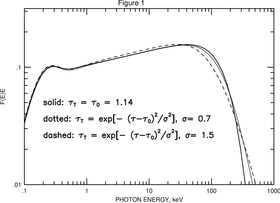
Figure 3.1: The spectrum resulting from co-adding the components due to different magnetic flares with a Gaussian distribution in the Thomson optical depth (see text), centered on $\tau_{0}=1.15$ with a width $\tau_{\sigma}=0.7$ (long-dashed curve) and $1.5$ (short-dashed curve). The spectrum from a single flare with optical depth $\tau_{T}=\tau_{0}$ is shown as a solid curve. The curves are normalized to the same integrated flux. These spectra demonstrate that current observations may not be able to differentiate between a single-flare spectrum and one comprised of many different flares if their optical depth is in the range $\sim 0.5-2$.

Figure (3.1) shows the results of our calculation for $\tau_{0}=1.14$ and two values of $\tau_{\sigma}$: $0.7$ and $1.5$. The spectrum from a single flare (solid curve) with $\tau_{T}=1.14$ is also shown for comparison. It can be seen that the plot for $\tau_{\sigma}=0.7$ is hardly distinguishable from that for $\tau_{T}=1.14$ (i.e., $\tau_{\sigma}=0$). Moreover, these curves differ the most above $100$ keV, where the OSSE data typically have error bars larger than this difference (see, e.g., Fig. 1 in Zdziarski et al. 1996). On the basis of this simple test, we would expect that Seyfert spectra may be comprised of contributions from many ARs encompassing a range ($0.5-2$) of $\tau_{T}$. We note, however, that a broader range in $\tau_{T}$ is unlikely because of the considerable flattening to the spectrum for $\tau_{\sigma}>1.5$.

The conclusion that $\tau_{T}$ is allowed to vary within the range of $0.5-2$ is very important for the magnetic flare model, since it is otherwise difficult to see how different flares could produce exactly the same $\tau_{T}$. It may also happen that a flare evolves through many phases and that its Thomson optical depth therefore varies with time. However, these calculations demonstrate that as long as that variation is restricted to the range $\sim 0.5-2$, the resulting spectrum is consistent with the observations.

3.5 Conclusions

We have considered the consequences of imposing a pressure equilibrium on the active regions of Seyfert Galaxies, in addition to the more often studied energy equilibrium, under the assumption that the emission arises within energetic magnetic flares above the surface of a cold disk. We showed that if the energy is supplied to the X-radiating plasma by magnetohydrodynamic waves with a group velocity $\sim c$, then $\tau_{T}$ probably falls within the range $1-2$. The current X-ray/$\gamma$-ray observations are consistent with this range of Thomson optical depths. We conclude that magnetic flares on the surface of the cold disk remain a viable explanation for the spectra observed in Seyfert Galaxies. Alternative explanations, based on a gravitational confinement of the ARs, cannot account for the observed ‘universality’ in the value of $\tau_{T}$.

Chapter 4 Pressure-Ionization Instability in X-ray Reflection

4.1 Abstract

The spectrum of Seyfert 1 Galaxies is very similar to that of several Galactic Black Hole Candidates (GBHCs) in their hard state, suggesting that both classes of objects have similar physical processes. While it appears that the two phase accretion disk corona (ADC) model is capable of explaining the observations of Seyfert galaxies, recent work has shown that this model is problematic for GBHCs. To address the differences in spectra of Seyferts and GBHCs, we consider the structure of the ionized X-ray skin near an active magnetic flare. We show that the X-ray skin is subject to a thermal instability, similar in nature to the well known ionization instability of quasar emission line regions.

We find that for Seyfert Galaxies, the X-ray skin is allowed to reside on either the cold ($T\sim 10^{5}$ K) or the hot ($T\lower 2.15277pt\hbox{$\;\buildrel>\over{\sim}\;$}10^{7}$ K) stable branches of the solution, and that observations show that the former is the one that is chosen in reality. However, due to the much higher ionizing X-ray flux in GBHCs, the only stable solution for the upper layer of the accretion disk is that in which it is highly ionized and is at the Compton temperature ($\sim$ few keV). Using numerical simulations for a slab geometry ADC, we show that the presence of a transition layer, here modeled as being completely ionized, with an optical depth $\tau_{\rm tr}\lower 2.15277pt\hbox{$\;\buildrel>\over{\sim}\;$}1$ dramatically alters the reflected spectrum from that predicted by ADC models having a discontinuity between a cold disk and a hot corona. Due to the higher albedo of the disk, the thermal blackbody component is reduced, giving rise to a lower Compton cooling rate within the corona. Therefore, higher coronal temperatures and a corresponding harder X-ray spectrum, as compared to the standard ADC slab geometry models, are possible. A transition layer also leads to a reduction in other observable reprocessing features, i.e., the iron line and the X-ray reflection hump. We conclude that it is possible that the differences between the X-ray spectrum of GBHCs such as Cyg X-1 and that of a typical Seyfert Galaxy can be explained within a unifying model in which X-rays come from magnetic flares above a cold accretion disk.

4.2 Introduction

The X-ray spectra of Seyfert Galaxies and Galactic Black Hole Candidates (GBHCs) indicate that the reflection and reprocessing of incident X-rays into lower frequency radiation is an ubiquitous and important process. For Seyfert Galaxies, the X-ray spectral index hovers near a “canonical value” ($\sim 0.95$; Pounds et al. 1990, Nandra & Pounds 1994; Zdziarski et al. 1996), after the reflection component has been subtracted out of the observed spectrum. It is generally believed that the universality of this X-ray spectral index may be attributed to the fact that the reprocessing of X-rays within the disk-corona of the two-phase model leads to an electron cooling rate that is roughly proportional to the heating rate inside the active regions (AR) where the X-ray continuum originates (Haardt & Maraschi 1991, 1993; Haardt, Maraschi & Ghisellini 1994; Svensson 1996). It has been suggested that the ARs are probably magnetically dominated structures, i.e., magnetic flares (Haardt et al. 1994; see also Galeev, Rosner & Vaiana 1979).

Although the X-ray spectra of GBHCs are similar to that of Seyfert galaxies, they are considerably harder (most have a power-law index of $\Gamma\sim 0.7$), and the reprocessing features are less prominent (Zdziarski et al. 1996). Dove et al. (1997) recently showed that a Rossi X-ray observation of Cygnus X-1 shows no significant evidence of reflection features (if the continuum is modeled as a power-law with an exponential cutoff). It is the relatively hard power law (and therefore the required large coronal temperature) and the weak reprocessing/reflection features that led Dove et al. (1997, 1998), Gierlinski et al. (1997) and Poutanen, Krolik & Ryde (1997) to conclude that the two-phase accretion disk corona (ADC) model, in both patchy and slab corona geometry cases, does not apply to Cygnus X-1.

One of the main problems with this model is that no self-consistent coronal temperature is high enough (for a given coronal optical depth) to produce a spectrum as hard as that of Cyg X-1 (Dove, Wilms, & Begelman 1997). This result is sensitive to the assumption that the accretion disk is relatively cold, such that $\sim 90$% of the reprocessed coronal radiation is re-emitted by the disk as thermal radiation (with a temperature $\sim 150$ eV). It is this thermal radiation that dominates the Compton cooling rate within the corona. However, if the upper layers of the accretion disk were highly ionized, creating a “transition layer,” a smaller fraction of the incident coronal radiation would be reprocessed into thermal radiation (i.e., the albedo of the disk would be increased), and therefore the Compton cooling rate in the corona would be reduced. Furthermore, as shown by Ross, Fabian & Brandt (1996; RFB96 hereafter), Auger destruction of the fluorescent iron line photons may explain the weakness of observed iron line features in Cyg X-1.

In this Chapter, we extend the earlier work of Nayakshin & Melia (1997a), who investigated the X-ray reflection process in AGNs assuming that the ARs are magnetic flares above the disk. We show that for parameters appropriate for both Seyfert galaxies and GBHCs, there should be a thermal instability at the surface of the cold disk. For AGNs, this thermal instability drives the gas in the X-ray skin down to temperatures $T\sim$ few$\times 10^{5}$ K. For GBHCs, however, the instability leads to the gas climbing up to $T\sim$ a few $\times 10^{7}$ K, the Compton temperature with respect to the coronal radiation field. This high temperature then explains why the X-ray skin of GBHCs should be much more strongly ionized as compared to AGN.

In §4.7, we explore the ramifications of this highly ionized transition layer on the energetics of the corona, and investigate how it alters the spectrum of the escaping radiation. We also discuss whether slab geometry ADC models, when transition layers are included, can account for the observed spectra of GBHCs. Our conclusions are such that, although a transition layer does allow for higher coronal temperatures, global two-phase, slab-geometry ADC models still cannot have coronal temperatures high enough to explain the data. However, a model having a patchy corona rather than a global corona appears very promising. Thus, it is possible that due to the thermal instability of the surface of the accretion disk, which leads to different endpoints for GBHCs and Seyfert galaxies, the X-ray spectra from these two types of objects can be explained by a single unifying ADC model.

4.3 Why a Transition Layer?

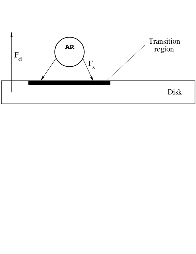
Figure 4.1: The geometry of the active region (AR) and the transition layer. Magnetic fields, containing AR and supplying it with energy are not shown. Transition region is defined as the upper layer of the disk with Thomson depth of $\sim$ few, where the incident X-ray flux is substantially larger than the intrinsic disk flux

We aim to determine the ionization structure of the disk atmosphere for the case when the X-ray flux originates in a magnetic flare. The relevant geometry is show in Figure (4.1). Since the flux of ionizing radiation from the active region is proportional to $1/d^{2}\times\cos i\propto d^{-3}$, where $i$ is the angle between the normal of the disk and the direction of the radiation and $d$ is the distance between the active region and the position on the disk, the ionization state of the disk surface will vary across the disk, and consequently only the regions near the active regions (with a radial size $\sim$ a few times the size of the active region, situated directly below the active region) may be highly ionized. To distinguish these important X-ray illuminated regions from the “average” X-ray skin of the accretion disk (i.e., far enough from active magnetic flares), we will refer to these regions as transition layers or regions. Most reprocessed coronal radiation will take place in these regions, and, in addition, most radiation emitted by the disk that propagates through the active regions will have been emitted in their vicinity. Therefore, in this Chapter, we will only consider the structure of the cold disk in the transition layer and only solve the radiation transfer problem for these regions as well.

Although a proper calculation of the ionization state of the transition layer is preferred, the complexity of this problem is not matched by any of the X-ray photoionization codes currently available in the literature. The difficulty is that the density of the transition layer is coupled to the radiation field, and therefore the ionization structure, thermal structure, and the radiation field must be solved self-consistently. Such a problem is outside the scope of this paper. Instead, we simply provide an order of magnitude estimate of the properties of the ionization layer to motivate the importance of the problem for a more elaborate future study.

4.4 Pressure Equilibrium

In this section, we show that the radiation pressure due to coronal radiation from an active region is very large, and then estimate the resulting pressure of the transition region. For transient flares, as opposed to a static corona, the X-ray flux from magnetic flares can only persist for a disk hydrostatic time scale (roughly one Keplerian rotation). Using the model of Svensson & Zdziarski (1994; SZ94 hereafter), we find that the photon diffusion time across the disk is much longer than the hydrostatic time scale for both radiation and gas-dominated disks. Therefore, no thermal equilibrium can be established between the underlying cold disk and the incident X-radiation during the flare. Nevertheless, since the optical depth of the X-ray skin is small compared to total optical depth through the disk, the radiation diffusion time scale and the atomic processes time scales are much shorter than the disk hydrostatic time scale (RFB96). Accordingly, the skin itself will be in quasi-equilibrium with the incident X-radiation.

The two-phase model with magnetic flares was put forward by Haardt & Maraschi (1991, 1993) and Haardt et al. (1994) to explain spectra of Seyfert Galaxies. The key assumptions of the model are (i) during the flare, the X-ray flux from the active region greatly exceeds the disk intrinsic flux, and (ii) the compactness parameter $l$ of the active region is large, so that the dominant radiation mechanism is Comptonization of the disk thermal radiation. The free-free compactness parameter of the particles in the AR is $l_{\rm ff}\simeq 3\times 10^{-3}\tau_{T}^{2}\Theta^{1/2}$, where the Thomson optical depth of the active region $\tau_{T}\lower 2.15277pt\hbox{$\;\buildrel<\over{\sim}\;$}1$, and the dimensionless electron temperature $\Theta\sim 0.3$ are reasonable numbers to explain X-ray observations of either GBHCs or Seyfert Galaxies. Therefore, assuming the luminosity due to bremsstrahlung radiation is negligible is equivalent to assuming $l\gg 0.01$.

The compactness parameter of the active regions is defined as

$$l\equiv{F_{\rm x}\sigma_{T}\Delta R\over m_{e}c^{3}},$$ (4.1)

where the size of the active region $\Delta R$ is thought to be of the order of the accretion disk height scale $H$ (e.g., Galeev et al. 1979), estimated here from the gas pressure dominated solution of SZ94,

$$\frac{H}{R}=7.5\times 10^{-3}(\alpha M_{1})^{-1/10}r^{1/20}[\dot{m}J(r)]^{1/5}[\zeta(1-f)]^{1/10},$$ (4.2)

where $\alpha$ is the viscosity parameter, $M_{1}\equiv M/10{\,M_{\odot}}$ is the mass of the black hole, $f$ is the fraction of accretion power dissipated into the corona (averaged over the whole disk), $r$ is the radius relative to the Schwarzschild radius, $J(r)=1-(3/r)^{1/2}$, and $\zeta$ is a constant of order unity (see §2.3). Therefore, the X-ray flux is approximated by

$$F_{\rm x}\,=\,3.6\times 10^{23}\,l\,\alpha^{1/10}M_{1}^{-9/10}\left({\dot{m}\over 0.05}\right)^{-1/5}(1-f)^{-1/10}{\rm erg\ cm}^{-2}\,{\rm sec}^{-1}.$$ (4.3)

The coronal energy dissipation fraction $f$ should be thought of as the surface-average fraction of energy transferred from the cold disk into the patchy corona above it. For the case of Cyg X-1, most of the bolometric luminosity seems to be in the hard X-ray band (e.g., Gierlinski et al. 1997). The corona then needs to process most of the disk power, i.e., $f\sim 1$ (Haardt and Maraschi 1991; Stern et al. 1995). In deriving equation (4.3), we took the location of the flare to be at $R=6R_{g}$ from the black hole, where the energy generation rate of the disk is a maximum. Throughout this Chapter, this position will be assumed implicitly.

We now compare the X-ray flux incident on the accretion disk with the intrinsic disk flux $F_{\rm d}$. The intrinsic flux is given by equation (2.2). We assume the dimensionless accretion rate $\dot{m}=\eta\dot{M}c^{2}/L_{\rm Edd}\sim 0.05$, a value thought to be appropriate for Cyg X-1. Here, $\dot{M}$ is the accretion rate, $\eta=0.056$ is the efficiency for the standard Shakura-Sunyaev disk, and $L_{\rm Edd}$ is the Eddington luminosity. Note that this definition of $\dot{m}$ is different by factor $\eta$ from that used by SZ94 (i.e., $\dot{m}\simeq 17\times\dot{m}_{\rm SZ94}$). We obtain for the disk intrinsic flux

$$F_{\rm d}=1.0\times 10^{22}M_{1}^{-1}\left({\dot{m}\over 0.05}\right)(1-f)\;{\rm erg\ cm}^{-2}\,{\rm sec}^{-1}{\rm.}$$ (4.4)

The illuminating X-ray flux is much larger than the intrinsic disk emission at regions that are near an active magnetic flare if $1-f\ll 1$ and the compactness parameter $l\gg 0.01$. For future reference, we also define the disk compactness parameter as $l_{\rm bb}\equiv F_{\rm d}\sigma_{T}H/(m_{e}c^{3})$:

$$l_{\rm bb}=0.03\left({\dot{m}\over 0.05}\right)^{6/5}\left(1-f\right)^{11/10}\left(\alpha M_{1}\right)^{-1/10}{\rm.}$$ (4.5)

(Note that instead of finding $F_{\rm x}$ through its connection with $l$, we could have required the magnetic flares to have a small covering fraction $f_{c}\ll 1$ and $1-f\ll 1$, and then we would have been able to deduce $F_{\rm x}\sim F_{\rm d}f/(1-f)f_{c}^{-1}\gg F_{\rm d}$ and $l\gg l_{\rm bb}$. In other words, to describe magnetic flares, one specifies either $l$ or $f_{c}$.)

We first consider the pressure of the disk surface layer before the occurrence of a flare (or, equivalently, far enough from the flare). If we assume that the upper layer of the disk with Thomson optical depth $\tau_{x}\sim 3$ is in hydrostatic equilibrium with the vertical gravitational force, the pressure $P_{0}$ in that region is approximated as

$$P_{0} \simeq {GMm_{p}\over R^{2}}\tau_{x}\,{H\over R}=6.2\times 10^{10}\;M_{1}^{-11/10}\alpha^{-1/10}$$ (4.6)

$$\times\tau_{x}\,\left({\dot{m}\over 0.05}\right)^{1/5}(1-f)^{1/10}\;{\rm erg\ cm}^{-3},$$

where $R=6R_{\rm g}$ (SZ94). When the flare turns on, the ratio of the incident radiation ram pressure to the unperturbed accretion disk atmosphere pressure is

$${F_{\rm x}\over cP_{0}}\,=\,2.\times 10^{2}\;l\,\tau_{x}^{-1}\,\left(\alpha M_{1}\right)^{1/5}\,\left({\dot{m}\over 0.05}\right)^{-2/5}(1-f)^{-1/5}{\rm,}$$ (4.7)

i.e., much higher than unity. Note that this conclusion is also applicable to flares in AGN. Thus, due to the equation (4.7) and the fact that $F_{\rm x}\gg F_{\rm d}$, the dynamical properties of the disk atmosphere will be strongly affected by the irradiating flux, as long as there is an active magnetic flare nearby, and this flux should be taken into account when solving the disk ionization structure.

It is possible that a wind is induced by the X-ray heating. However, the maximum gas temperature obtained due to the X-ray heating is the Compton temperature ($\lower 2.15277pt\hbox{$\;\buildrel<\over{\sim}\;$}10^{8}$ K) and is still far below the gas virial temperature ($kT_{\rm vir}\simeq GM/R$) for $R\lower 2.15277pt\hbox{$\;\buildrel<\over{\sim}\;$}10^{5}R_{g}$. Therefore, as shown by Begelman, McKee & Shields (1983), a large scale outflow cannot occur for $R\lower 2.15277pt\hbox{$\;\buildrel<\over{\sim}\;$}10^{4}R_{g}$. On the other hand, a local expansion of the gas is still possible, since the Compton temperature is higher than the the disk temperature. The maximum energy flux due to the wind, local evaporation or any mechanical expansion of the gas is $F_{\rm ev}\sim Pc_{s}$, where $P$ is the gas pressure in the transition region, and $c_{s}$ is its sound speed. Since $P\lower 2.15277pt\hbox{$\;\buildrel<\over{\sim}\;$}F_{\rm x}/c$, and $c_{s}\lower 2.15277pt\hbox{$\;\buildrel<\over{\sim}\;$}3\times 10^{-3}\,c$, we obtain ${F_{\rm ev}/F_{\rm x}}\lower 2.15277pt\hbox{$\;\buildrel<\over{\sim}\;$}3\times 10^{-3}$. Therefore, mechanical processes cannot cool the gas efficiently, and we neglect the influence of the possible wind on the energetics of the two-phase model. Note that evaporation of the material from the transition region could obscure the flare, but the large radiation flux from the flare is likely to push the gas laterally, away from the flare. This effect needs to be quantified in the future, but for now we assume that the flare is not obscured by the evaporation of the material. Below, we estimate the structure of the transition layer using the pressure and energy equilibrium conditions.

4.5 The Thermal Instability

Thermal instability was discovered by Field (1965) for a general physical system. He introduced the “cooling function” $\Lambda_{\rm net}$, defined as the difference between cooling and heating rates per unit volume, divided by the gas density $n$ squared. Energy equilibria correspond to $\Lambda_{\rm net}=0$. He argued that a physical system is usually in pressure equilibrium with its surroundings. Thus, any perturbations of the temperature $T$ and the density $n$ of the system should occur at a constant pressure. The system is unstable when

$$\left({\partial\Lambda_{\rm net}\over\partial T}\right)_{P}<0,$$ (4.8)

since then an increase in the temperature leads to heating increasing faster than cooling, and thus the temperature continues to increase. Similarly, a perturbation to a lower $T$ will cause the cooling to exceed heating, and $T$ will continue to decrease.

In the context of the transition layer stability, however, the constant pressure condition may be of lesser importance than the energy equilibrium in the following sense. Since the energy is being supplied by the coronal radiation, the thermal time scale $t_{\rm th}$ is the light crossing time of the transition region. The hydrostatic time, i.e., the time scale for balancing out pressure perturbations $t_{\rm h}$ in the layer, is given by the sound crossing time, which is at least a factor of $10^{3}$ longer than the thermal time scale (since $T<10^{8}$ K). Thus, in any perturbation, the energy equilibrium condition $\Lambda_{\rm net}=0$ is reached very quickly, whereas the pressure balance may be perturbed. The instability will exist if perturbing the gas density $n$ to a higher value will be followed by a decrease in pressure in that region, since then the gas will contract further because of the pressure imbalance with its surroundings. In other words, the condition for the transition layer instability is

$$\left({dP\over dn}\right)_{\Lambda_{\rm net}=0}<0{\rm,}$$ (4.9)

where the derivative is taken with condition $\Lambda_{\rm net}=0$ satisfied due to the short thermal time scale. Working through some simple algebra, one finds that

$$\left({dP\over dn}\right)_{\Lambda_{\rm net}=0}={P\over n}\,\left({\partial\Lambda_{\rm net}\over\partial T}\right)_{P}\left({\partial\Lambda_{\rm net}\over\partial T}\right)_{n}^{-1}{\rm.}$$ (4.10)

It is a rare occasion that the last multiplier on the right hand side is negative, and under most circumstances the conditions given by equations (4.9) and (4.8) are equivalent.

When studying ionization balance, it is convenient to define two parameters. The first one is the “density ionization parameter” $\xi$, equal to (Krolik, McKee & Tarter 1981)

$$\xi={4\pi F_{\rm x}\over n}\,.$$ (4.11)

The second one is the “pressure ionization parameter”, defined as

$$\Xi={F_{\rm x}\over 2cnkT}\equiv\frac{P_{\rm rad}}{P},$$ (4.12)

where $P$ is the gas pressure. This definition of $\Xi$ is the one used in the ionization code XSTAR (see below), and is different by a factor $2.3$ from the original definition of Krolik et al. (1981), who used the hydrogen density instead of the electron density. Ionization equilibria depend most sensitively on the density ionization parameter $\xi$, rather than $F_{\rm x}$ or $n$ separately. Solving the ionization and energy equilibrium gives the functions $T(\xi)$ and $\Xi(\xi)$. The latter one can be written as $\Xi(T)$ using the former. In terms of these variables, one can write $(dP/dn)_{\Lambda=0}=(d\Xi/dT)\,(\xi/\Xi)\;(\partial T/\partial\xi)$. In our calculations, we always found that $(\partial T/\partial\xi)>0$, so that the instability criterion (4.9) is equivalent to

$$\left({d\Xi\over dT}\right)_{\Lambda_{\rm net}=0}\,<0.$$ (4.13)

We now apply the X-ray ionization code XSTAR (Kallman & McCray 1982, Kallman & Krolik 1986) the problem of the transition layer. A truly self-consistent treatment would involve solving the radiation transfer in the optically thick transition layer, and in addition, finding the distribution of the gas density in the transition layer that would satisfy pressure balance. Since the radiation force acting on the gas depends on the opacity of the gas, this is a difficult non-linear problem. Thus, we defer such a detailed study to future work, and simply solve (using XSTAR) for the local energy and ionization balance for an optically thin layer of gas in the transition region. We assume that the ionizing spectrum consists of the incident X-ray power-law with the energy spectral index typical of GBHCs in the hard state, i.e., $\Gamma=1.5-1.75$, exponentially cutoff at 100 keV, and the blackbody spectrum from the cold disk below the transition layer. If the energy and ionization balance is found to be unstable for this setup, the transition layer will also be unstable.

When applying the code, one should be aware that it is not possible for the transition region to have a temperature lower than the effective temperature of the X-radiation, i.e., $T_{\rm min}=(F_{\rm x}/\sigma)^{1/4}$. In the spirit of a one zone approximation for the transition layer, we should use an average X-ray flux $\langle F_{\rm x}\rangle$ as seen by the transition region, which we parameterize as $\langle F_{\rm x}\rangle=0.1F_{\rm x}/q_{1}$, where $q_{1}=q/10$, and $q$ is a dimensionless number of order 10 (see figure 4.1; $F_{\rm x}$ is the X-ray flux at the active region). Using equation (4.3),

$$T_{\rm min}\simeq 5.0\times 10^{6}\;l^{1/4}\,q_{1}^{-1/4}\,\left({\dot{m}\over 0.05}\right)^{-1/20}\,\alpha^{1/40}\,M_{1}^{-9/40}\,\left[1-f\right]^{-1/40}.$$ (4.14)

The reason why simulations may give temperatures lower than $T_{\rm min}$ for a low ionization parameter $\xi$ is that in this parameter range XSTAR neglects certain de-excitation processes, which leads to an overestimate of the cooling rate (Zycki et al. 1994; see their section 2.3).

Figure 4.2: Gas temperature versus the pressure ionization parameter $\Xi$ – the ionization equilibrium curves for parameters appropriate for GBHCs. The incident spectrum is approximated by a power-law of photon index $\Gamma$, exponentially cutoff at $100$ keV, and the reflected blackbody with equal flux and temperature $T_{\rm min}$ (equation 4.14). Values of the parameters are: $\Gamma=$ 1.5, 1.75, 1.75, 1.7 and $kT_{\rm min}=$ 200, 100, 200, 400 eV, corresponding to the fine solid, thick solid, dotted and dash-dotted curves, respectively. The ionization equilibrium is unstable when the curve has a negative slope. In addition, there exist no solution below $T_{\rm min}$.

Figure 4.2 shows the results of our calculations for several different X-ray ionizing spectra. A stable solution for the transition layer structure will have a positive slope of the curve, and also satisfy the pressure equilibrium condition. As discussed in §4.4, $P\leq F_{\rm x}/c$ (i.e., $\Xi\geq 1$). In addition, if the gas is completely ionized, the absorption opacity is negligible compared to the Thomson opacity. Because all the incident X-ray flux is eventually reflected, the net flux is zero, and so the net radiation force is zero. In that case $P$ adjusts to the value appropriate for the accretion disk atmosphere in the absence of the ionizing flux (see also Sincell & Krolik 1996), which is given by equation (4.6). Therefore, the pressure ionization parameter should be in the range

$$1<\Xi<2\times 10^{2}\,l\left(\alpha M_{1}\right)^{1/5}\,\left({\dot{m}\over 0.05}\right)^{2/5}(1-f)^{-1/5}.$$ (4.15)

With respect to the ionization equilibria shown in Figure (4.2), the gas is almost completely ionized on the upper stable branch of the solution (i.e., the one with $T\lower 2.15277pt\hbox{$\;\buildrel>\over{\sim}\;$}10^{7}$ K), and thus the pressure equilibrium for such temperatures requires $\Xi\sim F_{\rm x}/cP_{0}\gg 1$.

In addition to the Compton equilibrium state, for some curves, there is a smaller stable region for temperatures in the range between $100$ and $200$ eV. The presence of this region is explained by a decrease in heating, rather than an increase in cooling (cf. equation 4.8 and recall $\Lambda_{\rm net}=$ cooling – heating). The X-ray heating decreases in the temperature range $100-200$ eV with increasing $T$ because of consecutive destruction (ionization) of ions with ionization energy close to this temperature region. Note that it is highly unlikely that the transition region will stabilize at the temperature $100$ – $200$ eV, because the effective temperature $T_{\rm min}$ is at or above this temperature range.

Figure 4.3: Gas temperature versus the pressure ionization parameter $\Xi$. The thick solid curve is same as that in Figure 4.2 and is appropriate for the hard state of a GBHC, whereas the two other curves are relevant to the soft state in GBHCs, or at large depth in the transition layer (see text). Values of the parameters are: $\Gamma=$ 2.1, 2.1 and $kT_{\rm min}=$ 200, 400 eV for the dotted and dashed curves, respectively.

Thus, although a fully self-consistent treatment of the pressure and ionization balance of the transition layer is needed to obtain exact results, it is very likely that the transition layer is highly ionized in GBHCs in the hard state for $\tau_{\rm x}\sim$ 1. The upper limit of $\tau_{\rm x}$ can only be found by a more exact treatment. In addition, the transition layer may be heated by the same process that heats the corona above it, albeit with a smaller heating rate. Furthermore, Maciolek-Niedzwiecki, Krolik & Zdziarski (1997) have recently shown that the thermal conduction of energy from the corona to the disk below may become important for low coronal compactness parameters and substantially contribute to the heating rate of the transition layer. Thus, the transition layer may be even hotter than that found by photoionization calculations.

Eventually, the X-rays are down-scattered and the radiation spectrum becomes softer as one descends from the top of the transition layer to its bottom. We can qualitatively test the gas ionization stability properties by allowing the ionizing spectrum to be softer than the observed spectrum of GBHCs in the hard state. In Figure 4.3 we show two examples of such calculations. The slope of the ionization equilibrium curve becomes positive everywhere above $kT\sim$ 100 eV, so that these equilibria are stable, and thus the gas temperature may saturate at $T\sim T_{\rm min}$, far below few keV, the appropriate temperature for the uppermost layer of the transition region. Thus, we know (see also §4.9) that the transition layer should terminate at some value of $\tau_{x}\sim$ few.

We also note that the thermal instability is not apparent in studies where the gas density is fixed to a constant value, regardless of its value. As shown by Field (1965), the thermal instability for the case with $n=$ const is always weaker than it is for the case of the system in pressure equilibrium. Following Field (1965), we argue that the assumption of a constant gas density is not justified for real physical systems, and that one always should use the pressure equilibrium arguments to determine the actual gas density and the stability properties of the system.

4.6 More Accurate Pressure Equilibrium

Summarizing the results learned from Figure (4.2), the transition layer is most likely at the Compton equilibrium state, although there is a narrow temperature range $T\sim 100-200$ eV (the “island” stable state) where the equilibrium state is possible if $T_{\rm min}<200$ eV. Let us now examine the pressure equilibrium arguments in more detail to discuss the stability properties of this state. Consider the pressure applied by incident X-rays on an optically thin layer of gas, $\tau_{x}\equiv n_{e}\sigma_{T}z\ll 1$:

$$P_{x}=n_{e}z\left(\sigma_{T}+\sigma_{a}\right){F_{\rm x}\over c}=\left(\tau_{x}+\tau_{a}\right){F_{\rm x}\over c}\ .$$ (4.16)

Here, $z$ is the vertical coordinate pointing up, $n_{e}$ is the local electron number density, $\sigma_{a}$ and $\tau_{a}$ are absorption cross section and optical depth, correspondingly ($\tau_{a}<1$ is implied). In the case of large optical depth, however, every photon incident on the layer interacts with the gas, thus passing its momentum to the layer. The radiation pressure then saturates at the radiation ram pressure $F_{\rm x}/c$. To take this effect into account, we can approximate the radiation pressure for all optical depths by

$$P_{x}={\tau_{x}+\tau_{a}\over 1+\tau_{x}+\tau_{a}}\,\,{F_{\rm x}\over c}\ .$$ (4.17)

Let us now come back to the transition layer problem. Within the optically thin layer, the pressure equilibrium condition is

$${dP_{\rm gas}\over dz}=-g_{0}n_{p}m_{p}-n_{e}\left\{\langle\sigma_{\rm x}\rangle-\langle\sigma_{\rm uv}\rangle\right\}{F_{\rm x}\over c}+n_{e}\langle\sigma_{\rm d}\rangle{F_{\rm d}\over c}\ .$$ (4.18)

Here, $g_{0}$ is the local gravity, which is approximately constant throughout the transition layer, equal to

$$g_{0}={GM\over R^{2}}\;{H\over R}\ .$$ (4.19)

We also define the “Roseland mean” cross sections for the three components of the radiation field in the transition region, i.e., the incident X-ray flux, the reflected UV (or soft X-ray in GBHC case) flux $F_{\rm uv}$, and the intrinsic disk emission $F_{\rm d}$. In particular, each of these cross sections is defined as

$$\langle\sigma_{i}\rangle\equiv{1\over F_{i}}\,\int dE{dF_{i}\over dE}\,\sigma_{i}(E)\ ,$$ (4.20)

where $E$ is the photon energy, and $i$ stands for either x, uv, or d. In the case at hand, $F_{\rm x}=F_{\rm uv}$ (although a part of the ”UV” flux can actually come out in the hard X-ray range, e.g., $10-20$ % may come out as the X-ray reflection component – see Magdziarz & Zdziarski 1995, for example), and $F_{\rm x}\gg F_{\rm d}$, so that we will neglect $F_{\rm d}$ for now. We will consider situations when $F_{\rm d}$ is non-negligible in §5.4.

In the spirit of a one-zone approximation, we may integrate equation (4.18) in the $z$-direction to obtain

$$P_{\rm gas}\simeq P_{0}+A{F_{\rm x}\over c}\ ,$$ (4.21)

where $P_{0}$ is the unperturbed pressure of the accretion disk atmosphere, given by equation (4.6) and we introduce the dimensionless constant $A$, which describes the effects of the radiation pressure on the transition layer. Following the discussion just before equation (4.17), $A$ is

$$A={\tau_{x}+\tau_{x}^{\prime}\over 1+\tau_{x}+\tau_{x}^{\prime}}\,-\,{\tau_{x}+\tau_{uv}\over 1+\tau_{x}+\tau_{uv}}\ ,$$ (4.22)

where $\tau_{x}^{\prime}\equiv\langle\sigma_{\rm x}\rangle n_{e}z$, $\tau_{uv}\equiv\langle\sigma_{\rm uv}\rangle n_{e}z$. Note that this expression now takes into account the most important features of the pressure equilibrium for the transition layer. In particular, $A$ is always smaller than unity; and, most significantly, it also takes into account the fact that when $\langle\sigma_{\rm uv}\rangle>\langle\sigma_{\rm x}\rangle$, the radiation pressure actually points up rather than down. Thus, the pressure equilibrium of the transition layer can be much more restrictive than that given by the simple estimate $\sim F_{\rm x}/c$, and we should compute the gas opacities to treat the pressure equilibrium correctly. We can also write down the pressure ionization parameter found using the estimate (4.21) for the gas pressure:

$$\Xi=\left[{P_{0}c\over F_{\rm x}}+\,A\right]^{-1}\ .$$ (4.23)

Figure 4.4: (a): Solid curve shows the ionization equilibrium curve. Using that equilibrium, the pressure equilibrium argument (equation 4.23) is used to estimate the corresponding ionization parameter. For the three pressure equilibrium curves the parameters are: $\tau_{x}=0.5$, 1, 2 and $P_{0}c/F_{\rm x}=$ $0.1$, 0.03 and 0.03 for the dashed, dotted and long-dashed curves, correspondingly. A stable configuration of the transition layer is achieved at the location where the ionization and pressure equilibrium cross. The gas absorption opacities are shown in panel (b). The solid curve is the X-ray opacity $\langle\sigma_{\rm x}\rangle$, whereas the dotted curve depict the UV-opacity $\langle\sigma_{\rm uv}\rangle$.

Figure (4.4 (a)) shows the ionization equilibrium together with approximate equilibrium given by equations (4.22,4.23), for one of the curves shown in (4.2). We tested several different values of $\tau_{x}$ and $P_{0}c/F_{\rm x}$. A stable solution is obtained when the solid curves intercepts one of the other curves, at which point ionization, energy and pressure equilibrium conditions are satisfied. As previously, regions with negative slope of the solid curve are thermally unstable, and temperatures lower than $T_{\rm min}=100$ eV are forbidden. Notice that only for relatively low Thomson depths of the transition layer the pressure equilibrium curve intercepts the island stable state. We doubt that a transition layer with such a low value of $\tau_{x}\simeq 0.5$ could be formed in reality, and thus we do not expect that the island state is truly stable, at least for magnetic flares in GBHCs. The X-ray spectra of GBHCs in the hard state contain most of the energy in the very hard X-ray band. Since the X-ray absorption is negligible above $\sim 10$ keV, these photons will not scatter until a Thomson depth of $\lower 2.15277pt\hbox{$\;\buildrel<\over{\sim}\;$}1$ is reached. After the first scattering, when these hard photons loose a considerable (almost all) fraction of their energy, they become vulnerable to the X-ray absorption below 10 keV, and can be finally absorbed. Therefore, $\tau_{x}$ less than 1 – 2 seems to be unrealistic.

The two curves that do not intercept the island state, with $\tau_{x}=$ 1 and 2, meet with the ionization equilibrium curve only at the Compton equilibrium state. Panel (b) of Figure (4.4) shows the gas temperature and the X-ray and UV mean absorption cross sections in units of the Thomson cross section for the same tests. One can observe that X-ray absorption is larger than the UV absorption, and thus the net radiation pressure force points down to the cold disk, but both of these absorption opacities become very small for $T\lower 2.15277pt\hbox{$\;\buildrel>\over{\sim}\;$}200$ eV. To a first approximation, since material is highly ionized for these conditions, the opacity is given by the Thomson opacity only. Since the reflected UV flux is equal to the ionizing X-ray flux, this implies that these two fluxes almost cancel each other in terms of the radiation pressure on the gas. So, the coefficient $A$ in equation (4.23) is very small and the effect of gravity is actually larger than the X-radiation pressure for these conditions. Thus, the pressure equilibrium curves saturate at $\Xi=F_{\rm x}/cP_{0}$ for high temperatures.

Rounding this discussion up, we believe that the only stable configuration available for the transition layer of GBHCs in the hard state is the one at the local Compton temperature. Future work should concentrate on finding not only the exact value of $\tau_{x}$, but the exact distribution of gas temperature, density and ionization state in the atmosphere of the accretion disk as well. For now, however, we will treat $\tau_{x}$ as a free parameter and numerically investigate the ramifications of the transition layer on the spectrum of escaping radiation and the physical properties of the corona in the next section.

4.7 “Three-Phase” Model

4.7.1 Physical Setup

As is clear from the foregoing discussion, there is an urgent need to explore the structure of the ionized transition region and how it affects the X-ray spectrum from magnetic flares. Since one depends on the other, this is a non-linear problem, and a very difficult one. At this point, however, we feel it will be useful to make a parameter search even in the context of a simplified model, where the accretion disk below the flare is broken into two regions: (i) the completely ionized transition region, and (ii) the cold accretion disk, which emits blackbody radiation at a specified temperature. By computing the X-ray spectrum from a magnetic flare above the transition layer with a range of $\tau_{\rm trans}$, we will try to determine whether there is a value of $\tau_{\rm trans}$, physically plausible enough, which would lead to the X-ray spectrum at least qualitatively close to the observed hard spectrum of Cyg X-1. If this turns out to be the case, then a future more detailed and accurate comparison of spectra from magnetic flares and Cyg X-1 spectrum will be forthcoming.

Gierlinski et al. (1997) have attempted to fit the broad-band spectrum of Cyg X-1 with active regions above a cold accretion disk. From this work, and the analysis below, it can be seen that the most difficult issue for the two-phase model is the too small observed lack of significant reprocessed soft X-radiation. For example, Zheng et al. (1997) showed that Cyg X-1’s luminosity in the hard state below 1.3 keV is about $5\times 10^{36}$ erg/s, whereas the luminosity above 1.3 keV is $\sim 3-4\times 10^{37}$ erg/s. This is impossible in the context of the simple two-phase corona-disk model, since about half of the X-radiation impinges on the cold disk and gets reprocessed into blackbody radiation. Accordingly, the minimum luminosity in soft X-rays below 1.3 keV should be about that of the hard component. Thus, the focus of our attention here will be the reprocessed radiation and not the active region intrinsic spectrum. This allows us to first use a simple radiation transfer code for the AR and yet retain most of the physics. Even though the geometry of the AR is probably closer to a sphere or a hemisphere than a slab, we shall adopt the latter for numerical convenience, neglecting the boundary effects. Experience has shown that spectra produced by Comptonization in different geometries are usually qualitatively similar (i.e., a power-law plus an exponential roll-over), and it is actually the fraction of soft photons entering the corona that accounts for most of the differences in the various models, because it is this fraction that affects the AR energy balance.

Following the standard practice in ionization/reflection calculations, we model the reflecting medium as being one dimensional, with its only dimension being the optical depth into the disk (measured from the top). The X-radiation enters the transition region through its top. In this region, the only important process taken into account is Compton interactions. After being down-scattered (but not absorbed, since iron ions are assumed to be completely ionized!), X-radiation is “incident” on the cold accretion disk from the bottom of the transition layer. The incident spectrum is reflected and reprocessed in the standard manner, and then re-enters the transition layer from below. Specifically, the reflected spectrum is given by the reflection component (Magdziarz & Zdziarski 1995) and the blackbody component due to the disk thermal emission. The blackbody emission is normalized such that the incident flux from the transition region is equal to the sum of the fluxes from the reflection component and the blackbody. The optically thick cold disk is held at a temperature $T_{\rm bb}=2.4\times 10^{6}$ Kelvin, and the blackbody spectrum is renormalized to produce the correct energy conserving flux.

The gas in the active region is heated uniformly throughout the region with a given heating rate (which is normalized to give the assumed compactness for the region). The gas is cooled by Compton interactions with radiation re-entering the active region from below (Compton interactions are the dominant cooling mechanism for these conditions). To crudely take the geometry into account, we permit only a part of the reprocessed radiation to re-enter the corona, and fix this fraction at $0.5$ (cf. Poutanen & Svensson 1996). The Thomson optical depth of the corona is fixed at $\tau_{\rm c}=0.7$ to avoid complications with pair production, which will be included in later work. Further, we shall see below that the compactness of the active regions is limited to a relatively small number, i.e., $l\lower 2.15277pt\hbox{$\;\buildrel<\over{\sim}\;$}$ few, so that pair production may simply be irrelevant for real flares.

We employ the Eddington (two-stream) approximation for the radiative transfer in both the AR and the transition layer, using the zero (isotropic) and the first order moments of the exact Klein-Nishina scattering kernel (Nagirner & Poutanen 1994). The transition region and the AR are divided into some number of zones, such that the Thomson optical depth of each zone does not exceed 0.1. The energy balance for the transition region within the scope of our approximate treatment is given by requiring the gas to be at the Compton temperature, and is solved separately for each zone. The latter is important for a moderately optically thick transition region, since then we find the region to be stratified in temperature due to a change in the local radiation field as one moves from the bottom to the top of the layer. Since our code is time-dependent, we simply start with some “reasonable” initial conditions and then allow the Active Region, the transition region and the radiation field to come into equilibrium.

According to the physical setup of this problem, the observed spectrum consists of the direct component, emerging through the top of the AR, and a fraction of the reflected radiation that emerges from the transition layer and does not pass through the corona on its way to us. This fraction is chosen to be 0.5 as well. Physically, it accounts for the fact that, as viewed by an observer, a part of the transition region itself is blocked by the active region. The overall setup of the active region - disk connection is very similar to the one used by Poutanen & Svensson (1996), except for the addition of a transition layer above the cold disk.

4.7.2 Results

Figure 4.5: Resulting spectrum from the patchy corona disk model as a function of the Thomson optical depth $\tau_{\rm trans}$ of the transition layer. The layer is assumed to be completely ionized. Notice that higher values of $\tau_{\rm trans}$ lead to a harder spectrum with the disk blackbody component progressively smaller.

Figure (4.5) shows the “observed” spectrum for several values of $\tau_{\rm trans}$: $0$, $0.6$, $2.5$, and $10$, with $\Omega=0.5$. It can be seen that the spectrum hardens as $\tau_{\rm trans}$ increases. To help explain why this happens, we plot in Figure (4.6) the integrated albedo $a$ for photons with energy $E>1$ keV as a function of $\tau_{\rm trans}$. The albedo is simply the ratio of the returning flux in the given energy range to the incident one. The returning flux is the one that emerges from the top of the transition layer. As $\tau_{\rm trans}$ increases, a large fraction of the photons from the AR are reflected before they have a chance to penetrate into the cold disk where the blackbody component is created. Therefore, a smaller flux of energy is deposited below the transition layer, which leads to a decreased cooling from the Comptonization of soft, reprocessed radiation. For a moderate optical depth $\tau_{\rm trans}$, this result is quite insensitive to the temperature in the transition layer as long as Fe is highly ionized. We checked this by simply setting the transition temperature at the arbitrarily chosen values of $1.5$ and $6$ keV, instead of the self-consistent temperature distribution calculated above, which varied (with optical depth into the transition layer) from about $2$ to $4$ keV for the respective values of $\tau_{\rm trans}$. We found that the relative variations in the spectrum and the albedo resulting from this were less than about $3\;\%$. For higher optical depths ($\tau_{\rm trans}\lower 2.15277pt\hbox{$\;\buildrel>\over{\sim}\;$}4$), pre-Comptonization of the soft disk radiation becomes important and additionally decreases the Compton cooling of the corona by this component, so that the temperature of the transition layer becomes essential.

Figure 4.6: Integrated albedo (reflected fraction) as a function of the transition layer optical depth, $\tau_{\rm trans}$, for photons with energy $>1$ keV. Also plotted (dotted curve) is the ratio of the observed hard luminosity (above $2$ keV) to the observed total luminosity.

Figure 4.7: Decomposition of the observed spectrum (solid curve) into its essential components: the intrinsic AR spectrum (short-dash) plus the reflected component (emerging from the top of the transition layer; dotted curve) multiplied by $\Omega=0.5$. The observed spectrum for the case of $\tau_{\rm trans}=0$ is also shown by the long-dashed curve for comparison (shifted for clarity). See text for a further discussion.

Figure (4.7) shows the observed spectrum (solid curve), comprised of the intrinsic AR spectrum (short-dash) and the reflected component (emerging from the top of the transition layer; dotted curve) multiplied by $\Omega=0.5$. Also shown for comparison is the observed spectrum for the case of $\tau_{\rm trans}=0$ (long-dash). All the intensities propagate in the upward direction. Notice that due to the presence of the transition layer, the reflected component is much harder than the reprocessed component, which would be the “normal” reflection/reprocessing component without this layer. Notice also that the bump around $\sim 40$ keV normally attributed to the reflected component is broad (compared with the long-dashed curve), and so the reflected component is here less noticeable.

Furthermore, the combined power below $2$ keV accounts for only $25\;\%$ of the total, whereas the corresponding fraction is about $50\;\%$ in the standard (static) two-phase model. This large power coming out in low energy photons was the main reason why the standard two-phase corona-disk model failed to account for the observations of Cyg X-1 (e.g., Gierlinski et al. 1997)

4.8 Tests with a Non-Linear Monte Carlo routine

The Eddington approximation for radiative transfer in the corona and the transition layer is rather inaccurate for optically thin cases. It means that the results presented in the previous section cannot be trusted quantitatively, i.e., one may not use them to produce a fit to some observed spectra. We thus would like to check our approximate code with one of the best existing codes on the Comptonization and energy balance of the corona. Namely, we use the slab-geometry ADC model of Dove, Wilms, & Begelman (1997), which uses a non-linear Monte Carlo (NLMC) routine to solve the radiation transfer problem of the system. The free parameters of the model are the seed optical depth $\tau_{e}$ (the optical depth of the corona excluding the contribution from electron-positron pairs), the blackbody temperature of the accretion disk and its compactness parameter, $l_{\rm bb}$, and the heating rate (i.e., the compactness parameter), $l_{\rm c}$, of the ADC. The temperature structure of the corona is determined numerically by balancing Compton cooling with heating, where the heating rate is assumed to be uniformly distributed. The $e^{-}e^{+}$-pair opacity is given by balancing photon-photon pair production with annihilation. Reprocessing of coronal radiation in the cold accretion disc is also treated numerically. For a more thorough discussion of the NLMC routine, see Dove, Wilms, & Begelman (1997). The transition layer is treated identically to the corona, accept here the heating rate is set to zero. Therefore, the transition layer, numerically modeled using 8 shells, each with equal optical depth ${\rm d}\tau=\tau_{tr}/8$, will obtain the Comptonization temperature due to the radiation field from both the corona and the accretion disk.

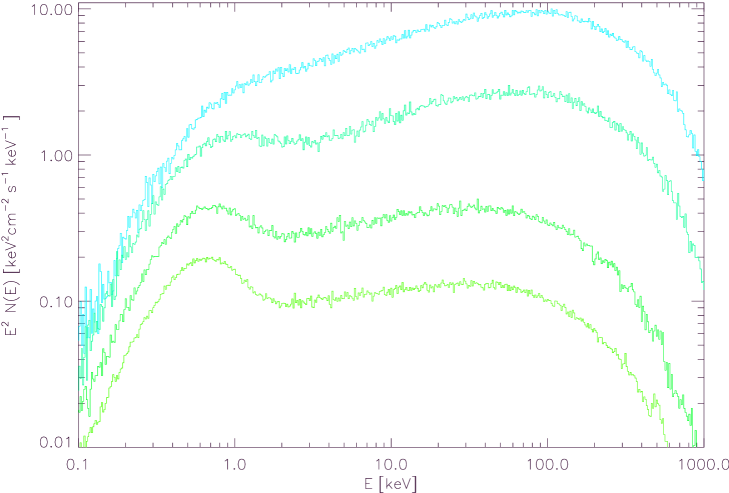
Figure 4.8: The predicted spectrum for various values of the transition layer optical depth computed with the non-linear Monte-Carlo code. Planar geometry is assumed. From top to bottom, $\tau_{\rm tr}=10,5,2.5,$ and $1.0$.

The model contains three regions: (1) A cold accretion disk, assumed here to have a temperature $kT_{\rm min}=150$ eV, (2) the transition layer, situated directly above the cold disk, and (3) the corona, situated directly above the transition layer. Plane parallel geometry is assumed. In Figure 4.8, we show the resulting broad band spectra for the model parameters tested. This figure is to be compared with figure (4.5) obtained with the Eddington approximation code. We found that the latter was systematically off in the energy balance for the corona, i.e., it was always hotter than found by the NLMC code. However, the qualitative behavior of the system is the same in both codes, which is what we expected. We plan to use the NLMC code in future work to attempt to fit some actual spectra of GBHCs and AGN. For all models in Figure 4.8, $l_{\rm c}=2$, $l_{\rm bb}=0.01$, $kT_{\rm min}=150$ eV, and $\tau_{c}=0.3$. These parameters correspond to the model producing the maximum corona temperature. In contrast to models in which $\tau_{\rm tr}=0$, the corona temperature for a given value of $\tau_{c}$ is not simply a function of $l_{\rm c}/l_{\rm bb}$. To see this, consider the case where $\tau_{tr}\gg 1$. Here, the albedo of the disk is essentially unity, and therefore all of the soft photons emitted will be from the intrinsic flux of the disk (no reprocessing). Therefore, setting $l_{\rm bb}\ll 1$ yields the maximum coronal temperatures possible. Note that the maximum temperature levels out as $\tau_{tr}\rightarrow\infty$. Although, in this limit, there is no reprocessing of hard X-rays in the cold disk, there is still “reprocessing” in the transition layer. As $\tau_{tr}$ increases, more coronal radiation is down-scattered to the Compton temperature of the transition layer, which is $kT_{tr}\sim 1-4$ keV. Even at these temperatures, Compton cooling of this “reprocessed” radiation in the corona is very efficient.

It is interesting to note that, only for $\tau_{\rm tr}\lower 2.15277pt\hbox{$\;\buildrel>\over{\sim}\;$}10$, the coronal temperature is high enough such that the corresponding spectrum of escaping radiation is hard enough to describe the observations of Cyg X-1. (The canonical value of the photon power-law of Cyg X-1 is $\Gamma=1.7$; for $\tau_{c}=0.3$, this power law corresponds to $kT_{c}\sim 150$ keV). It is probably unphysical, however, to assume the transition layer is completely ionized for such large optical depths. In fact, the numerical model for $\tau_{\rm tr}=10$ predicts a temperature of $kT_{\rm tr}\sim 500$ eV near the bottom of the layer. Therefore, even with the advent of transition layers, it still appears unlikely that a global slab geometry ADC model can have self-consistent temperatures high enough to reproduce the observed hard spectra of Cyg X-1 and other similar GBHCs.

4.9 Discussion

By considering the irradiated X-ray skin close to an active magnetic flare above a cold accretion disk, we have shown that solutions for the skin equilibrium structure found with the usual assumption of a constant gas density are unstable in a broad range of parameter state. When the pressure equilibrium is taken into account, one finds that two stable states (one cold and one hot) are possible. For the case of GBHCs, we showed that the low temperature equilibrium state is forbidden due to a high value of the ionizing flux. Thus, the X-ray irradiated skin of GBHCs must be in the hot equilibrium configuration, where the gas is at the local Compton temperature ($kT\sim$ few keV) with the radiation field from both the corona and the cold disk. In fact, even for global ADC models of GBHCs, such a transition layer is found to be likely.

The transition layer may be thought of as a partially transparent mirror. Crudely, some of the photons are scattered back without a change in energy, and the rest proceed to the cold disk and suffer the usual transformation into soft disk photons. This effect changes the integrated albedo of the transition layer, so that a smaller fraction of the incident X-rays is used to create the soft radiation that is the dominant source of cooling in the two-phase model. In addition, the Compton down-scattering in the transition layer does not contribute to the cooling because the energy gained by an electron in the layer is later used to up-scatter the softer photons coming from the cold disk (whereas without the transition layer this energy would be used to produce the soft radiation).

This reduction in X-ray reprocessing yields a lower Compton cooling rate within the corona, and higher coronal temperatures than previous ADC models are allowed. Using the NLMC routine, we have found that for global ADC models with $\tau_{\rm c}\sim 0.3$, the coronal temperature can be as high as $\sim 150$ keV if the optical depth of the transition layer is $\tau_{\rm tr}\lower 2.15277pt\hbox{$\;\buildrel>\over{\sim}\;$}10$. These coronal properties are what is needed to explain the X-ray observations of GBHCs such as Cyg X-1. In addition, for $\tau_{\rm trans}\gg 1$, the predicted reprocessing features as well as the thermal excess should be substantially smaller than that of previous ADC models in which the transition layer was not considered. This reduction of the reprocessing features is crucial for the model being consistent with the observations of GBHCs (e.g., Gierlinski et al. 1997, Dove et al. 1998).

It is interesting to note that if magnetic flares have the same geometry and compactness in GBHCs as they do in AGN, the existence of the transition layer means that GBHC spectra should be harder than those in typical Seyfert 1s (where the layer is non-ionized, see Chapter 5). Further, for $\tau_{\rm trans}\gg 1$, the spectrum may be somewhat different from that of single cloud Comptonization plus a standard cold reflection component, because the reflection component here is broadened by scatterings in the transition layer. It is possible that this effect explains Gierlinski et al.’s (1997) finding that the Cyg X-1 spectrum cannot be fit with one component.

The observed soft X-ray excess should contain comparatively less power than the hard component, in contrast to Seyfert 1s. The difference is caused by the difference in the X-ray reflection albedo $a$, since the fraction of the energy reflected as the soft disk radiation is $(1-a)$. The albedo is only $10-20$ % in Seyferts (e.g., Magdziarz & Zdziarski 1995), whereas we found the albedo for GBHCs to be as large as $a\sim 0.75$, which still may be not the highest possible, since a further testing with a range of geometries is needed. The relatively small disk emission is consistent with observations of Cyg X-1, but was listed as one of the primary problems with the two-phase model by Gierlinski et al. (1997), who used the standard X-ray reflection formula (i.e., with $a\sim 0.1-0.2$).

Note also that the Thomson optical depth of the flares should be similar in GBHCs and Seyfert Galaxies, and therefore so should the electron temperature within their ARs (see Chapter 3; this aspect of the model does not depend on $M$).

Gierlinski et al. (1997) found that an anisotropy break (that is not seen in Cyg X-1 data) is always present in the patchy two-phase model. As was discussed in Poutanen & Svensson (1996), the anisotropy break occurs where the second order scattering (of the disk radiation in the corona) peaks. However, as we found from our numerical results, the anisotropy break disappears as the optical depth of the transition layer increases. The reason for this is the following: the reprocessed continuum is no longer the blackbody emission (which was assumed by Gierlinski et al. 1997, and Poutanen & Svensson 1996) and is quite broad. Compton scattering broadens any initial photon distribution, and therefore the second order scattering of the reprocessed continuum becomes a very diffuse function, with a shallow peak. Among other effects that should reduce the anisotropy break is the variance of the temperature of the disk emission with distance from the flare (which we neglected here in one-zone approximation). The cold disk emission will then be a sum of blackbodies with different temperatures, and will be even broader than what we obtained in our calculations. Finally, since the overall spectrum is a sum from flares with a distribution of temperatures and the optical depths (see §3.4), second order scattering will mean different amplification factors for the soft photons entering different flares, which will further dilute the break. Thus, we believe that earlier contrasting results found by Gierlinski et al. (1997) are due to an over-simplification of the magnetic flare model physics.

The reflected component in the observed spectrum must be less pronounced or not observable, depending on the transition layer optical depth, which is again consistent with observations (e.g., Zdziarski et al. 1996).

Most of the hard X-rays do not penetrate through the transition layer, and the spectrum gets softer as it approaches the cold disk. The Iron K$\alpha$ line, small to start with due to the small amount of reprocessing of coronal radiation, is completely smeared out by the time the radiation escapes the system. No line photons are created in the transition layer itself, because we found that the Compton equilibrium state typically resides at the ionization parameter $\xi\lower 2.15277pt\hbox{$\;\buildrel>\over{\sim}\;$}10^{4}$, whereas no fluorescent iron line emission is produced for $\xi\lower 2.15277pt\hbox{$\;\buildrel>\over{\sim}\;$}5\times 10^{3}$ (Matt, Fabian & Ross 1993, 1996). The observed weak K$\alpha$ line may then be arising from the cold outer disk. The same is true for the Fe edge. Note that observationally, it is very hard to detect a broad Fe edge in the case of Cygnus X-1 (Ebisawa 1997, private communication).

Thus, as far as we can see, observations of the hard state of the GBHCs do not rule out magnetic flares as the source of X-rays, and instead support this theory. Earlier findings on the contrary were affected by the use of assumptions that magnetic flares or the X-ray reflection process in GBHCs cannot deliver. Furthermore, it appears that the observed X-ray spectrum of Cyg X-1 can be explained by the transition optical depth of $\sim 3$, which is physically plausible, and that, apart from the self-consistent difference in the structure of the transition layer, the same parameters for magnetic flares might be used in both AGN and GBHCs to explain their spectra.

The spectral calculations reported here could also be appropriate for the static patchy corona model if the upper layer of the disk were hotter than usually assumed. Indeed, it is not hard to imagine that the upper layer is being heated in a way similar to heating of the Solar corona. If the temperature of the layer is few keV and its Thomson optical depth is close to $\sim 3$, then the spectra produced in this situation may be close to the observed hard spectra of the GBHCs. This possibility does not appear to have been explored by previous workers. At the same time, even if such a static model could remove the problems for the GBHCs spectra, one would need to explain why the upper layer of the disk in Seyfert Galaxies is not being heated in a similar manner. Thus, the real strength of the magnetic flare model of the active regions is in the fact that this is the same physics that explains the spectra of both Seyfert Galaxies and GBHCs.

Chapter 5 X-ray reflection in AGNs and The BBB

5.1 BBB in Seyfert Galaxies and the Transition Layer

The UV to soft X-ray spectrum of many Active Galactic Nuclei (AGNs) may be decomposed into a non-thermal power-law component and the so-called Big Blue Bump (BBB), which cuts off below about 0.6 keV (e.g., Sanders et al. 1989). A major obstacle in constraining the characteristics of the BBB has been that it lies in the difficult to observe EUV and very soft X-ray region. In recent years, however, there has been considerable progress in this direction (e.g., Walter & Fink 1993; Walter et al. 1994; Zhou et al. 1997). The observed spectral shape of the bump component in Seyfert 1’s hardly varies, even though the luminosity $L$ ranges over 6 orders of magnitude from source to source. Walter et al. (1994) concluded that the cutoff energy $E_{c}$ of the BBB (when fitted as a power-law with exponential rollover) is very similar in different sources whose luminosities vary by a factor of 10⁴. Note that we here will refer to the results of the second method of fitting the spectral shape of the bump suggested by these authors, i.e., using prescription (B) (see their §4.2). The first prescription (A) assumes that the ultraviolet to the far ultraviolet spectral slope remains constant, which is contrary to what one would expect based on our model of the accretion disk emission. In this model, the far-UV component is due to reprocessing in the transition region of the X-rays from magnetic flares (as elaborated below in this Chapter), and has no relation to the intrinsic disk emission, which should show up at the disk effective temperature of $\sim$ few eV. Thus, it is important to allow the reprocessed spectrum and the disk intrinsic emission to vary with respect to one another in the fits, and prescription (B) satisfies this criterion better than prescription (A). Although the data of Walter et al. (1994) were not precise enough to distinguish between different emission mechanisms, Walter et al. (1994) pointed out that if the variations in the ratio of the soft X-ray excess to UV flux from one object to another are interpreted as a change in the temperature of the BBB, then this change is smaller than a factor of 2. Confirming conclusions follow from the work of Zhou et al. (1997).

Early theoretical work on the BBB spectrum focused on the role of optically thick emission from the hypothesized accretion disk surrounding the central engine (e.g., Shields 1978; Malkan & Sargent 1982; Czerny & Elvis 1987; Laor & Netzer 1989). However, this mechanism is now facing several obstacles (e.g., Barvainis 1993; Mushotzky et al. 1993). An alternative model, in which the BBB is interpreted as thermal, optically thin free-free radiation, has been proposed by Antonucci & Barvainis (1988), Barvainis & Antonnuci (1990), Ferland et al. (1990), and Barvainis (1993). There are strong arguments against this emission mechanism as well (Malkan 1992).

It seems to us that the observations Walter & Fink (1993) and Walter et al. (1994) are difficult to interpret in the terms of accretion disk thermal emission. AGNs are thought to accrete both from their nearby environments via the Bondi-Hoyle process and from the tidal disruption of stars, though over time, the former is dominant (e.g., Melia 1994). At least initially, the accretion rate is therefore $\dot{M}\propto M^{2}$, where $M$ is the black hole mass, but this constitutes a runaway process in the sense that $L/L_{Edd}\propto t$, where $t$ is the time, and $L_{Edd}$ is the Eddington luminosity. When $L\rightarrow L_{Edd}$, the outward radiation pressure presumably suppresses the inflow, with the effect that $L$ saturates at the value $\sim L_{Edd}\propto M$. A second argument in favor of the supposition that the ratio $L/L_{Edd}$ is relatively independent of $M$ is the fact that we observe very similar X-ray spectra for objects of very different luminosities (e.g., Zdziarski et al. 1996), for otherwise the disk structure would differ from source to source, giving rise to different spectra. As a statistical average, we thus expect that $L\propto M$.

In view of this, let us next examine how the various different emission mechanisms fare in their prediction of the BBB cutoff energy $E_{c}(L)$. For any radiation process, the flux $F$ scales as $L$ over the emitting area, which itself scales as $M^{2}$. Thus, in general we expect that $F\propto L^{-1}$. The blackbody flux is $F_{\rm bb}=\sigma T^{4}$, where $T$ is the effective temperature, and so $T\propto L^{-1/4}$. Thus, when $L$ varies by 4 orders of magnitude, it is expected that $T$ ought to itself vary by a factor of 10. This is not consistent with the observations discussed above. Further, the disk effective temperature is

$$T_{\rm eff}\simeq 3\times 10^{4}\,M_{8}^{-1/4}\,\dot{m}_{-2}^{1/4}\left[(1-f)\right]^{1/4}\,{\rm K}\ ,$$ (5.1)

where $\dot{m}_{-2}\equiv\dot{m}/0.01$. This temperature is considerably smaller than the roll-over energies ($E_{c}\sim 50-80$ eV) in the BBB emission found by Walter et al. (1994).

A more sophisticated treatment of the disk structure in its inner region shows that the scattering opacity may dominate over the absorptive one, and thus the emission spectrum may differ from that of a blackbody. For example, the disk may radiate as a ‘modified blackbody’ (Rybicki & Lightman 1979), for which the flux is then given by

$$F_{\rm mb}\sim 2.3\times 10^{7}T^{9/4}\rho_{d}^{1/2}{\rm\,erg}\;{\rm\,cm}^{-2}\;{\rm\,s}^{-1}{\rm,}$$ (5.2)

where $\rho_{d}$ (in ${\rm\,g}\;{\rm\,cm}^{-3}$) is the disk mass density and $T$ is in Kelvins. For accretion disks, $\rho_{d}\sim M^{-1}$ (e.g., §2.3), and so $T\sim M^{-2/9}$, which again is not consistent with the data, if $L$ is in general proportional to $M$. We believe that more complicated emission mechanisms, i.e., accretion disk atmosphere calculations, are unpromising as well because the emission will always be characterized by some sort of temperature, either equal to $T_{\rm eff}$ or some function of it, and we see no physical reason why this temperature would not vary with $\dot{m}$ and $M$. These last two quantities most likely vary by orders of magnitude for different sources in any large sample of QSO or Seyferts. Our conclusion is thus that the BBB emission does not come from the accretion disk intrinsic emission.

5.2 The Thermal Ionization Instability for AGN

We now discuss the thermal instability (Chapter 4) of the surface layer for AGN. The most important distinction from GBHC case is the much higher mass of the AGN, and thus an ionizing X-ray flux is smaller by $\sim 7$ orders of magnitude (see equation 4.3). The minimum X-ray skin temperature is again approximated by setting the blackbody flux equal to the incident flux, assumed to be $q\sim 10$ times less than the escaping coronal flux. The gas pressure dominated solutions gives

$$T_{\rm min}\simeq 1.5\times 10^{5}\,l^{1/4}\,\alpha^{1/40}\,M_{8}^{-9/40}\left[{\dot{m}\over 0.005}\right]^{-1/20}\,\left(1-f\right)^{-1/40}\,\left({q\over 10}\right)^{-1/4}\,{\rm,}$$ (5.3)

whereas the radiation-dominated one yields

$$T_{\rm min}\simeq 7.\times 10^{4}\,l^{1/4}\,M_{8}^{-1/4}\left[{\dot{m}\over 0.05}\right]^{-1/4}\,\left(1-f\right)^{-1/4}\,\left({q\over 10}\right)^{-1/4}\,\ .$$ (5.4)

These estimates show our main point right away: the lower X-ray flux density in AGN may allow the transition layer to saturate at either the cold equilibrium state or the “island” state, whereas that was not possible for GBHCs. To investigate this idea, we ran XSTAR as described in Chapter 4, but for parameters appropriate for the AGN transition layer. In particular, we accepted that the disk blackbody emission temperature is $6$ eV (cf. equations 5.3 & 5.4), and that the gas density is $10^{17}$ cm^-3. The X-rays illuminating the transition region are assumed to mimic the typical Seyfert hard spectra, i.e., a power-law with photon index $\Gamma=1.9$ and the exponential roll-over at 100 keV. The ratio of the X-radiation ram pressure to the X-ray skin unperturbed pressure is chosen to be correspondingly higher $F_{\rm x}/cP_{0}\sim 10^{2}-10^{3}$ (see equation 4.7; we also believe that $\dot{m}\lower 2.15277pt\hbox{$\;\buildrel<\over{\sim}\;$}0.05$ for typical Seyferts, as explained in Chapter 6). As explained earlier in §4.5, XSTAR produces inaccurate results below $T\sim T_{\rm min}$, so that these regions of the ionization equilibrium curve should be disregarded. To test sensitivity of our results to the parameters of the X-ray spectrum, we also ran a case for $kT_{\rm bb}=12$ eV and the rollover energy at $200$ keV.

Figure 5.1: Same as Figure (4.4), but for the AGN transition layer. (a): Solid curve shows the ionization equilibrium curve. Using that equilibrium, the pressure equilibrium arguments are used to estimate the corresponding $\Xi$. For the three pressure equilibrium curves the parameters are: $\tau_{x}=0.5$, 1, 2 and $P_{0}c/F_{\rm x}=10^{-3}$, $10^{-3}$ and $10^{-2}$ for the dashed, dotted and long-dashed curves, correspondingly. A stable configuration of the transition layer is achieved at location where the ionization and pressure equilibrium curves cross. (b): the gas absorption opacities. The solid curve is the X-ray opacity $\langle\sigma_{\rm x}\rangle$, whereas the dotted curve depicts the UV-opacity $\langle\sigma_{\rm uv}\rangle$

We show results of these two simulations in Figures (5.1) and (5.2). Notice that the “cold” equilibrium branch, i.e., the region with $T\sim 10^{5}$ K is more stable than the island state. None of the pressure equilibrium curves intercepts the island state. The two curves with $\tau_{x}=0.5$ and $1$ do intercept the cold equilibrium state, but the more optically thick case with $\tau_{x}=2$ does not in Figure (5.1), whereas all the three curves intercepts the cold state in Figure (5.2). On both Figures, the horizontal lines are caused by the UV opacity exceeding the X-ray opacity for low and high temperature in one of the simulations, thus leading to the negative estimates of $\Xi$. Physically, it means that the UV pressure on the gas exceeds that of the incident X-rays, so that the net radiation force points upward. A wind may be induced in these temperature ranges (i.e., below $10^{5}$ and above $\sim 10^{7}$ K). Clearly, more detailed future work is needed to investigate the parameter space where the cold state is stable. However, its existence is required by observations of X-ray reflection and fluorescent iron lines in Seyferts, as we will enunciate in Chapter 7.

Figure 5.2: Same as Figure (5.1), but for the effective temperature $kT_{\rm bb}=12$ eV.

5.3 The Origin of the Big Blue Bump

As was elaborated in §5.1, there is no consistent explanation for the origin of the BBB, one of the most prominent features in the AGN spectra. We believe that our theory of the ionization pressure instability may offer a plausible explanation for the BBB emission. As the ionization equilibria calculations show, there is no stable solution for the transition region in the temperature range $2-3\times 10^{5}\lower 2.15277pt\hbox{$\;\buildrel<\over{\sim}\;$}T\lower 2.15277pt\hbox{$\;\buildrel<\over{\sim}\;$}10^{7}$ Kelvin (see Figure 5.1 and 5.2). Furthermore, temperatures below the effective temperature of the X-ray radiation are also forbidden. The only low temperature solution permitted by the stability analysis is the one with a temperature around $2\times 10^{5}$ Kelvin.

Notice that the Rosseland mean optical depth to the UV emission is of order 1 to a few for this temperature range, as seen from simulations (see panels (b) in figures 5.1 and 5.2). The radiation spectrum produced by the transition layer will be either a blackbody spectrum, or a modified blackbody (with recombination lines as well, of course). This spectrum may explain the observed roll-over energies in the BBB emission from Seyfert Galaxies (see references in §5.1) rather naturally. Since the moderately optically thick emission spectrum will saturate at photon energy of $\sim 2-4\times T$, $T\sim 2\times 10^{5}$ provides an excellent match to the observed roll-over energies of $\sim 40-80$ eV.

As one can check using Field’s (1965) stability criterion, the transition layer radiating via blackbody emission is thermally stable. Furthermore, even the modified blackbody emission mechanism stabilizes the instability. This consideration shows that the transition layer will be even more stable in the cold state in the realistic optically thick calculation, which would take into account spectral reprocessing of the incident spectrum. Further, notice that effective temperature $T_{\rm eff}$ cannot be seriously lower than $T_{\rm eff}\simeq 1\times 10^{5}$ Kelvin. The point here is that the compactness parameter in the two-phase patchy corona model cannot be much lower than unity (see §2.4 and equations 5.3 & 5.4).

Thus, the temperature of the BBB is fixed by the atomic physics, in particular by the fact that many atomic species have ionization potential close to 1 Rydberg, which corresponds to a temperature of $T\simeq 1.5\times 10^{5}$ K. This temperature turns out to be independent of the number of magnetic flares, and so it is independent of the X-ray luminosity of the source, as found by Walter & Fink (1993) and Walter et al. (1994).

5.4 The X-ray Baldwin effect

Here we will present a simple argument to demonstrate how our theory of the ionized transition layer may account for the recent observation of the X-ray Baldwin effect. Namely, it has been found (Nandra et al. 1997) that all AGNs that are very luminous in the X-ray band (i.e., $L_{\rm x}>10^{44}-10^{45}$ erg/sec in the 2-10 keV window) show little or no Iron line emission, in sharp contrast to lower luminosity AGNs. This is not easily understood without invoking an instability, as explained in the following citation of A. C. Fabian (1998), which we received as a private communication:

”Nandra et al (1995, 1997) find no evidence for the iron line or any reflection features in most quasars. In the second paper, it is shown that the equivalent width of the iron line diminishes with source luminosity above about $10^{44}$ erg/sec and it is suggested that the disk is increasingly ionized, perhaps because the objects are closer to the Eddington limit. This is puzzling because the disk must jump from being ‘cold’ to completely ionized, otherwise there would be intermediate objects with even larger equivalent widths when the surface iron in the disk is H or He-like (Matt, Ross & Fabian 1994). There should at the same time be a deep broad iron edge which is not seen. (There is strong iron absorption in the reflection continuum in both a cold and an ionized disk, but it only shows up in the latter case because the lack of oxygen and iron-L absorption below the edge make the reflection continuum strong there.)

Possibly there is a jump between states caused by the way in which the corona is energized. When the Eddington ratio is low the magnetic field amplified by differential motions in the disk extracts most of the energy released to well above the disk. There is then little thermal energy release from within the disk and it is essentially cold and has a sharp surface for reflection purposes. When however the ratio is increased there may be a flip at some level to a somewhat thicker, radiation-pressure supported (inner) disk which has a fuzzy, highly-ionized surface (i.e. the density drops gradually with height into the corona). Studies of the behavior of disks in the Galactic Black Hole Candidates will be instructive here.”

We think that the pressure ionization instability described in this Chapter and Chapter 4 may be the process that explains the disappearance of the line. First, note that the energy equilibrium in most luminous AGN may push the transition layer over “the edge” of the stable cold solution (i.e., $\sim 3\times 10^{5}$ K) to the unstable region. The disk effective temperature is

$$T_{\rm eff}\simeq 1\times 10^{5}M_{8}^{-1/4}\,\dot{m}^{1/4}\left[(1-f)\right]^{1/4}\ .$$ (5.5)

The actual minimum temperature may even be higher than this estimate, since the accretion disk itself may become effectively thin for accretion rates $\dot{m}$ close to unity (see SZ94), and the emission may become a modified blackbody emission. A particular accretion disk model (with $\alpha$ and other parameters specified) and an exact treatment of the transition layer ionization, pressure and energy equilibria are needed to find the transition layer temperature, but it is rather natural to expect that this temperature may be larger than the disk effective temperature by a factor $\sim$ few. For example, Ross, Fabian & Minishige (1992) finds that the disk spectrum may be for some conditions better approximated by a Wien spectrum with $T=2.5T_{\rm eff}$. Thus, for accretion rates close to the Eddington-limited one, the transition layer temperature may be higher than $3\times 10^{5}$ K irrespectively of the strength of the X-ray coronal heating, which would make it impossible for the layer to be on the cold stable branch of the solution.

The next energetically stable solution exists above $T\sim 100$ eV (see Figure 5.1). It could be either the short “island” state, or could be the whole region of the curve upwards of $T\sim 100$ eV, since we found that for steeper X-ray illuminating spectra the $\sim 200$ eV $-1$ keV region may become stable. If the transition layer indeed was at this temperature range, the observations by Nandra et al. (1997) would be puzzling, since fluorescent iron line emission for $\xi\sim 500-5000$ is even stronger than it is for the cold stable state (Matt et al. 1993, 1996).

However, when the disk switches from a gas to a radiation-dominated solution, and when the disk intrinsic flux $F_{\rm d}$ becomes comparable to or larger than the X-ray flux $F_{\rm x}$ from the active region, the pressure equilibrium for the transition layer may be of a different nature than we found it to be in §4.6. Specifically, in the latter case we neglected the contribution of the intrinsic disk flux to the radiation pressure in the transition region, since $F_{\rm d}\ll F_{\rm x}$ was shown to be the case. Here, however, the disk intrinsic flux produces the main force on the gas in the transition layer. In fact, one can neglect the ram pressure of the incident X-radiation in this limit.

The unperturbed gas pressure in the transition region, $P_{\rm gas,s}$, can be found by first finding the overall pressure required to maintain the equilibrium (cf. equation 4.6), and then subtracting the radiation pressure due to the escaping disk flux $F_{\rm d}$:

$$P_{\rm gas,s}\simeq P_{0}-\tau_{d}F_{\rm d}/c={\tau_{x}\over 2}{F_{\rm d}\over c}\,\left[\zeta-2{\tau_{d}\over\tau_{x}}\ {\rm,}\right]$$ (5.6)

where $\tau_{d}$ is the Rosseland mean total optical depth of the transition layer to the escaping radiation, whereas $\tau_{x}$ is the Thomson optical depth. We have used standard accretion disk theory in the formulation of SZ94 to arrive at this expression. The parameter $\zeta$ is the parameter introduced by SZ94 to account for the uncertainty in the vertical averaging of the radiation diffusion out of the disk (see §2.3). Different authors use $\zeta$ ranging from $2/3$ to $2$. In any event, this estimate shows that, in the given case, the gas pressure may account for a tiny fraction of the transition region pressure (negative $P_{\rm gas,s}$ in equation 5.6 means that a wind will be induced, or the treatment needs to be refined to take into account radiation anisotropy, etc). We then have $P_{\rm gas,s}\ll F_{\rm d}$. Now, if $F_{\rm x}$ is not too much smaller than $F_{\rm d}$, then it also implies $\Xi=(F_{\rm x}/cP_{\rm gas,s})\gg 1$. For high values of $\Xi$, the only stable equilibrium is the Compton equilibrium, and here the transition layer is completely ionized. The latter fact can be the explanation for the absence of the iron lines in very luminous AGN.

We should also note that this goes in line with the finding of no BBB in high-luminosity AGNs of Zheng et al. (1996) and Laor et al. (1997), since, just as we found in the case of GBHCs (see Chapter 4, figures 4.5 and 4.8), the completely ionized transition layer with $\tau_{x}\lower 2.15277pt\hbox{$\;\buildrel>\over{\sim}\;$}1$ may reduce the reflected UV component. Since we also think that X-rays do not contribute the majority of power in luminous Radio Quiet AGN, the Big Blue Bump may be smeared and reduced to invisibility on the background of the dominant thermal disk emission.

Finally, it is also curious to note that since the disk effective temperature scales as $M^{-1/4}$, AGNs with $M\sim 10^{10}{\,M_{\odot}}$ may be cold enough that the transition layer (if the corona is full) once again may exist on the cold stable equilibrium solution, and the iron line may re-appear again, in line with the suggestions of Prof. Fabian.

5.5 Constraints on Magnetic Flares from X-ray reflection

Note that the spectral constraints limit the compactness parameter in both AGNs and GBHCs. In particular, for AGNs, we know that $T_{\rm eff}$ as given by equations (5.3) and (5.4) cannot exceed $\sim 2\times 10^{5}$ K. If $T_{\rm eff}$ was larger, the stable low temperature state would disappear, and the observations of a low ionization degree reflector and a cold neutral iron line in AGNs would be left unexplained by our theory. Thus, $l\sim 0.1-$ few in AGNs. Similarly, for GBHCs, the observed soft X-ray emission in the hard state of GBHCs can be fitted by a blackbody with a temperature $\simeq 150$ eV (see equation 4.14). This low temperature is only possible if $l$ is smaller than unity, and is as small as $0.1$. In principle, a better spectrum calculation of the X-ray reflection and the spectrum formation in the geometry of an active region is needed in order to set the upper limit on $l$. In any event, it is notable that the constraints on $l$ from AGNs and GBHCs observations are rather similar. We will use this fact when modelling the global spectral behavior of disks in Chapter 7, and will see that it leads to observationally testable predictions.

Chapter 6 Energy budget of the corona

6.1 Energetics of the magnetically-fed Corona

We shall now turn to the question of the global energy transport by magnetic flux tubes. This issue is very important, since observations of Seyfert Galaxies show that probably as much $\sim 50$% of the accretion power must be channeled to the corona, and yet it has never been shown that this can be accomplished by any particular energy transport mechanism. Furthermore, as we saw in Chapter 4, observations of GBHCs, if interpreted in the context of the two-phase model, require even larger portion of the energy to be transported out of the disk by magnetic flares, such that the global energy transport is dominated by magnetic energy flux. In fact, the energy balance issue is equivalent to the question of the normalization of the observed X-ray spectra, and as such is as important a test of the two-phase model as the shape of the spectrum itself. This test has never been conducted before.

The time-averaged magnetic energy flux (from inside the disk to the corona) $F_{\rm m}$ is

$$F_{\rm m}=v_{b}\langle{B^{2}\over 8\pi}\rangle{\rm,}$$ (6.1)

where $\langle B^{2}/8\pi\rangle$ is the volume average of the magnetic field pressure in the disk, and $v_{b}$ is the buoyant rise velocity, i.e., the average velocity with which a magnetic flux tube is rising due to buoyancy. It is well known that a magnetic field inside the accretion disk is an efficient mechanism for angular momentum transport in the disk (e.g., Shakura & Sunyaev 1973, Lightman & Eardley 1974, Hawley, Gammie & Balbus 1995). Therefore, it is thought that given a numerical value for the Shakura-Sunyaev $\alpha$-parameter, one may constrain the volume average magnetic field reasonably well. This conclusion comes from the fact that a magnetic field line resists in a known way the shearing resulting from the differential rotation of the disk. The relevant magnetic stress is $\langle B_{r}B_{\phi}/8\pi\rangle$, where $B_{r}$, $B_{\phi}$ are the $r$ and $\phi$ components of the magnetic field, respectively. This volume average is expected to be of the order of the average magnetic pressure in a turbulent medium. On the other hand, the component of the stress tensor responsible for the momentum transfer in the framework of the standard theory is $\alpha P_{\rm tot}$. Accordingly,

$$\langle{B^{2}\over 8\pi}\rangle\lower 2.15277pt\hbox{$\;\buildrel<\over{\sim}\;$}\alpha P_{\rm tot}\;.$$ (6.2)

The $<$ sign in this equation corresponds to a possible case when the so-called turbulent viscosity is larger than the magnetic viscosity, such that $\alpha$ is larger than that due to the magnetic field alone. Numerical simulations show that the turbulent and magnetic viscosities are of the same order (e.g., Stone et al. 1996), and we will assume that this is indeed true.

At the same time, with the standard prescription for viscosity, one can show that the local total energy flux $F_{\rm tot}$ (which is equal to the sum of the magnetic and radiation energy fluxes) is equal to $(9/8)\alpha c_{s}P_{\rm tot}$ (via equation 4.26 of Frank, King & Raine 1992, for example). The fraction of the power transported away from the disk by magnetic fields is then

$$f\equiv{F_{\rm m}\over F_{\rm tot}}\lower 2.15277pt\hbox{$\;\buildrel<\over{\sim}\;$}{v_{b}\over c_{s}}\;.$$ (6.3)

Thus, in order for the magnetic energy flux to amount to a significant portion of the total energy flux, the buoyant rise velocity $v_{b}$ should be almost equal to the gas sound speed $c_{s}$. Vishniac (1995a,b), however, found that $v_{b}$ cannot be as large as the sound speed. In fact, Vishniac (1995a,b) estimated that the magnetic energy out-flux only accounts for a fraction $\sim\alpha$ of the radiative energy transport. This conclusion may be expected to change in the case of strong magnetic flux tubes, with pressure comparable to the gas ambient pressure, because their Alfvén speed may be closer to $c_{s}$ (Vishniac 1997, private communication). Still, the fluid viscosity is not zero, which leads to a friction between rising flux tubes and the fluid, and the problem may be further complicated by interactions between the neighboring tubes as well as other factors (e.g., Parker 1979, Vishniac 1995a,b). It does not appear reasonable to us to suggest that $v_{b}$ can closely approach $c_{s}$, although it cannot be completely ruled out at this time. The hard spectrum of Cyg X-1, in any event, requires $f\simeq 0.8$ ans so can be accounted for (by the two-phase model) only if $v_{b}\simeq c_{s}$ – clearly an unphysical situation.

A possible solution to this theoretical difficulty lies in the fact that the above estimate of the volume average of the magnetic field (equation 6.2) is only correct for a diffuse magnetic field, and a similar argument carefully applied to the case where most of the field is localized to strong magnetic flux tubes allows the volume average magnetic field to be much larger than $\alpha P_{\rm tot}$, as we will now show. The reason to suspect that there may be a difference in the amount of the magnetic field resistance to the differential flow in these two cases is the following fact. The diffuse and tangled magnetic field will be strongly coupled to the fluid and thus will definitely take part in the differential rotation of the fluid, so it will be stretched and will contribute to the $\alpha$-parameter by resisting this stretching. At the same time, a flux tube is an entity of its own, which manifests itself in the fact that the tube can move with respect to the fluid, e.g., be buoyant. Accordingly, the flux tube may avoid the stretching by simply not following these motions of the fluid that try to deform the tube. We need to turn to some estimates to see if this is the case for accretion disks.

Consider a flux tube that is shaped as a torus with larger radius $a_{0}\lower 2.15277pt\hbox{$\;\buildrel<\over{\sim}\;$}H$, where $H$ is the disk vertical thickness, and the smaller radius $a$ ($\pi a^{2}$ is then the cross sectional area of the tube). Note that we are concerned here with a flux tube that is immersed in the accretion disk gas rather than a tube that has already risen to the top of the disk and is ready to produce a flare, because it is the former flux tube that carry the energy to the corona. Let us assume that without differential rotation (see below), the flux tube would be at some equilibrium state. In the accretion disk, the two opposite sides of the torus may be at different radii: $R$ and $\simeq R+a_{0}$. The gas at these radii moves with different Keplerian velocities, and thus the flux tube will be experiencing a shear force. The differential velocity $v_{d}$ between the two rings of matter separated by distance $a_{0}$ in the disk can be written as $v_{d}\simeq c_{s}(a_{0}/H)$. Now let us assume that the flux tube is not being stretched by the differential motion, that is, it moves with some average azimuthal velocity, as a solid body. There is a viscous drag force $D$ on the flux tube in this case, caused by the friction as the fluid flows by the tube. The magnitude of this force is

$$D\simeq C_{d}\rho v_{d}^{2}aa_{0}/2$$ (6.4)

(e.g., Parker 1979, §8.7, and references there), where $C_{d}$ is the drag coefficient. For the flux tube not to be deformed by the drag force, the tube magnetic tension should exceed this force. The flux tube tension force $T$ is given by

$$T={B^{2}\over 8\pi}\pi a^{2}\;.$$ (6.5)

The ratio of these two forces is

$${T\over D}\sim{2a\over a_{0}}C_{d}^{-1}{P_{\rm mag}\over P_{\rm tot}}\left(H\over a_{0}\right)^{2}\;,$$ (6.6)

where $P_{\rm tot}$ is the total disk pressure. For a relatively thick flux tube, we have $4a/a_{0}\lower 2.15277pt\hbox{$\;\buildrel<\over{\sim}\;$}1$. The drag coefficient is uncertain in this equation, since it depends on the level of the fluid viscosity and many other model dependent factors. The value typically used for this coefficient for conditions appropriate to accretion disks or stars is $C_{d}\sim 1/4$ (following Vishniac 1995; Stella & Rosner 1984; Sakimoto & Coroniti 1989; Parker 1979). With this value of the drag coefficient, equation(6.6) asserts that for flux tubes with magnetic field pressure comparable to the equipartition value, and the size $a_{0}$ smaller than the disk scale hight $H$, the magnetic field tension is larger than the drag force applied to the flux tube by the differential flow in the disk. The tube cannot be deformed by the flow in this case, and instead is dragged around almost as a solid body. The contribution of the flux tube to the momentum transfer is reduced by the ratio of the drag force $D$ to the tension force $T$. If all the magnetic field is in the form of strong flux tubes for which the magnetic tension exceeds the drag force, then the limits on the magnetic field volume average become

$$\langle{D\over T}P_{\rm mag}\rangle\lower 2.15277pt\hbox{$\;\buildrel<\over{\sim}\;$}\alpha P_{\rm tot}\;,$$ (6.7)

or, approximately, $\langle P_{\rm mag}\rangle\lower 2.15277pt\hbox{$\;\buildrel<\over{\sim}\;$}\alpha P_{\rm tot}\langle(T/D)\rangle$. Note that observations of the Sun suggest that as much as $\sim 90$% of the overall magnetic field is concentrated in strong magnetic flux tubes, at least on the surface (Parker 1979, §10.1); it therefore seems reasonable that most of the field in accretion disks is contained in the flux tubes too. Depending on the exact value of the typical flux tube size, $C_{d}$ and other uncertainties, the volume average of the magnetic field can be considerably larger than $\alpha P_{\rm tot}$. We can estimate the ratio of the magnetic energy flux $F_{\rm m}$ to the radiation energy flux as

$${f\over 1-f}\,\simeq{v_{b}\over c_{s}}{1+T\over D}\;{\rm,}$$ (6.8)

which is much easier to reconcile with the magnetic energy flux required by observations, since now the buoyant rise velocity can be comfortably below its absolute maximum value, i.e., the sound speed $c_{s}$ and yet provide a magnetic energy flux exceeding the radiation flux.

A simple physical analogy here is a sail on a ship. When the sail is “on”, the force (due to wind) acting on the sail is many times larger than it is in the case of the sail that is folded in. The amount of this wind-sail interaction clearly depends not on the overall mass of the sail, but on the state of the sail – whether it is open and positioned properly with respect to wind or whether it is rolled in a tube. Similarly, with the same volume average magnetic field one gets less or more interaction between differential flow and the field depending on whether the field is uniform in space, or contained within strong flux tubes, such that most of the flow simply misses the tubes to interact with them.

6.2 Radiation Pressure and Properties of a Single Flux Tube

In our consideration of the magnetic fields in the previous section, we did not explicitly separate the total pressure into the radiation pressure $P_{\rm rad}$ and the gas pressure $P_{\rm gas}$. This approach is practically always used in the literature (e.g., Galeev et al. 1979; Vishniac et al. 1995a,b and further references cited therein) mainly because of two reasons. The first one is that historically it is the Solar magnetic field phenomena that stimulated much of the work on magnetic fields in turbulent plasmas, and for the Solar interior conditions the radiation pressure is everywhere much smaller than the gas pressure. The second reason is a more pragmatic one: the problem becomes virtually intractable if the radiation pressure dominates, since one now has three interacting components instead of two. This approach (of neglecting the radiation pressure dynamical effects) is equivalent to the assumption that the radiation and particles move together, as one fluid, even when radiation pressure dominates over the gas pressure. It is clear that such an approach should indeed be valid as long as the scales of interest in the disk are much larger than the photon mean free path, since in this case the radiation is strongly coupled to particles due to the large opacity. Below we will attempt to quantify when such a “one fluid” approximation is valid and when it is not, and what are the implications for the magnetic flux tubes in the radiation dominated accretion disks.

To do so, we need to compare the time scale for the radiation diffusion into the flux tube with a time scale important for generation and maintenance of strong magnetic flux tubes. The radiation diffusion time scale $t_{\rm d}$ can be estimated as $t_{\rm d}\sim(a/c)n^{\prime}_{e}\sigma_{T}a$, where $n^{\prime}_{e}$ is the particle density inside the flux tube, which we can assume to be of the order of the disk particle density $n_{e}$, $\sigma_{T}$ is the Thomson cross section, and $a$ is the flux tube cross sectional radius.

Turbulent motions of the fluid are believed to be the mechanism for the magnetic field amplification (e.g., Vishniac 1995a,b). Let $u_{\rm t}$ be the typical turbulent velocity, and $\lambda_{\rm t}$ be the turbulent length scale (corresponding to the largest eddy length scale). The gas executes turbulent motions on the eddy turn over time scale $t_{\rm t}\equiv\lambda_{\rm t}/u_{\rm t}$. To see if diffusion is faster than turbulent motions, we compare the time scales $t_{\rm d}$ and $t_{\rm t}$:

$${t_{\rm d}\over t_{\rm t}}\sim{a^{2}\over H\lambda_{\rm t}}\,{u_{\rm t}\over c_{s}}{\tau_{d}c_{s}\over c}\;,$$ (6.9)

where $c_{s}$ is the gas sound speed, $H$ is the vertical scale height of the disk and $\tau_{d}$ is the disk Thomson optical depth. The scale of the flux tube $a$ is likely to be of the order of the scale of turbulent motions (Vishniac 1995a). Further, in the standard Shakura-Sunyaev viscosity prescription, the turbulent velocity and spatial scale are parameterized by $u_{\rm t}\lambda_{\rm t}=\alpha c_{s}H$. Finally, in the radiation pressure dominated region of the disk, the standard disk equations lead to $\tau_{d}c_{s}/c\simeq\alpha^{-1}$, for arbitrary radii and accretion rates. Therefore, one can see from Equation (6.9) that the ratio of the diffusion time scale to the turbulent time scale is of the order unity. This means that standard accretion disk equations permit radiation to diffuse into the flux tubes in the radiation dominated region of the disk. Moreover, we compared $t_{\rm d}$ with one eddy turn over time scale, whereas generation of the field comparable with the equipartition value is likely to take much longer, simply because one turbulent eddy does not carry enough energy. Due to this it is almost guaranteed that the diffusion of radiation into the flux tubes is much faster than the field generation process in the standard accretion disk theory.

What does this mean for a single magnetic flare? Since the radiation easily diffuses inside the flux tube, the radiation pressure inside the flux tube should be approximately equal to the ambient radiation pressure. It is then only the ambient gas pressure that can confine the flux tube side-ways, that is, $P_{\rm mag}\leq P_{\rm gas}$. In fact it is even not clear if accretion disks will produce magnetic flares of the same compactness parameter as it does in the gas-dominated case (see §6.3.3), i.e., whether the spectrum from a single magnetic flare will change or not.

Summarizing the ongoing discussion, it is clear that the magnetic fields in the radiation-dominated disks are either mostly in a diffuse form, or in the form of weak flux tubes, whose maximum pressure is given by the gas pressure. Weakness of the flux tubes in the radiation-dominated disk means that they will not behave as solid bodies anymore (see equation 6.6), and will be stretched by the differential flow just as diffuse magnetic fields are. Thus, one recovers the estimate $\langle P_{\rm mag}\rangle\lower 2.15277pt\hbox{$\;\buildrel<\over{\sim}\;$}\alpha P_{\rm tot}$, and the amount of energy deposited into the hard X-rays decreases as the accretion disk becomes radiation-dominated.

6.3 The Model Parameter Space

6.3.1 Dim State

We start by discussing very dim accreting disk systems, namely ones that accrete at such a low accretion rate $\dot{m}\lower 2.15277pt\hbox{$\;\buildrel<\over{\sim}\;$}\dot{m}_{d}$ that magnetic flux tubes cannot provide enough energy for the emitting regions to be compact. As was shown in §2.4, bremsstrahlung, rather than inverse Comptonization becomes the dominant emission mechanism when $l\lower 2.15277pt\hbox{$\;\buildrel<\over{\sim}\;$}0.01$. Setting $l$ to 0.01 in equation (2.14) gives us the estimate of the corresponding accretion rate:

$$\dot{m}_{d}\lower 2.15277pt\hbox{$\;\buildrel<\over{\sim}\;$}2\times 10^{-4}\,\alpha\,\zeta^{-1}\;.$$ (6.10)

Below this accretion rate, the X-ray spectra should be different from the standard Seyfert hard spectrum, since the two-phase model becomes invalid. Note that the disk is gas-dominated for these low accretion rates, and so the magnetic energy flux might be dominant over the radiation transport, and it is possible that the X-ray component may again be very prominent in the overall spectrum. However, studies of magnetic flare emission mechanisms in the regime $l\ll 1$ need to be done to test this situation further. We shall call this parameter space ‘dim’ accreting systems, and the most model independent statement that we can make at this time is that their spectra should be different than that of standard hard Seyfert spectra.

6.3.2 Hard State

Let us now move up in the accretion rate parameter space, such that the compactness parameter of the magnetic flares is $l\lower 2.15277pt\hbox{$\;\buildrel>\over{\sim}\;$}10^{-2}$, and the gas pressure dominates over that of the radiation in the disk, i.e. $\dot{m}_{d}\lower 2.15277pt\hbox{$\;\buildrel<\over{\sim}\;$}\dot{m}\lower 2.15277pt\hbox{$\;\buildrel<\over{\sim}\;$}\dot{m}_{\rm rad}$, where $\dot{m}_{\rm rad}$ is

$$\dot{m}_{\rm rad}=\dot{m}_{0}\,(1-f)^{-9/8}=2.2\times 10^{-3}\left(\alpha M_{8}\right)^{-1/8}\,(1-f)^{-9/8}{\rm,}$$ (6.11)

for AGN, and

$$\dot{m}_{\rm rad}=1.6\times 10^{-2}\left(\alpha M_{1}\right)^{-1/8}\,(1-f)^{-9/8}{\rm,}$$ (6.12)

for GBHCs. Svensson & Zdziarski [1994] showed that the transition from gas to radiation dominated regime is affected by transferring a fraction $f$ of the disk energy into the corona. Namely, they found that this transition happens at $\dot{m}_{\rm rad}=\dot{m}_{0}/(1-f)^{9/8}$, where $\dot{m}_{0}$ is the accretion rate when $P_{\rm rad}=P_{\rm gas}$ in the standard theory. However, this approach assumes that the fraction $f$ is itself a constant, which may not necessarily be the case. As we found earlier in this Chapter, the fraction $f$ decreases when $P_{\rm rad}$ exceeds $P_{\rm gas}$. If we are to use some guidance from observations of GBHC state transitions, we would have concluded that $\dot{m}_{\rm rad}$ is not greatly affected by the corona, since the state transitions seem to happen at $\dot{m}_{\rm rad}\simeq 0.05$ (see §7.6), and this (depending on the exact value of $\alpha$, which may be quite small) is just a factor $\sim 2-3$ higher than equation (6.12) predicts for a a 10 ${\,M_{\odot}}$ blackhole. If we re-scale $\dot{m}_{\rm rad}$ from $0.05$ for GBHCs using $\dot{m}_{\rm rad}\propto M^{-1/8}$, we obtain that $\dot{m}_{\rm rad}\simeq 0.007$ for Seyfert Galaxies with $M\sim 10^{8}{\,M_{\odot}}$.

Our discussion in §6.1 showed that it is possible for magnetic buoyancy to expel out of the disk more energy in the form of magnetic fields than the common radiation transport does in the gas-dominated accretion disks. At the same time, the approximate nature of the discussion may not yield an exact value for $f$. If we now again try to use some guidance from GBHCs, whose broad band spectra are better understood observationally than those of Seyferts, we will see that $f$ must probably be as large as $0.7-0.9$ to explain the hard spectra of some GBHCs (see Chapter 4).

To summarize, in the “hard” accretion rate parameter range, i.e., when $\dot{m}_{d}\lower 2.15277pt\hbox{$\;\buildrel<\over{\sim}\;$}\dot{m}\lower 2.15277pt\hbox{$\;\buildrel<\over{\sim}\;$}\dot{m}_{\rm rad}$, we expect that the spectrum is hard for both Seyferts and GBHCs, with the latter spectrum being harder than the former spectrum, due to the strongly ionized nature of the X-ray reflection in GBHCs (see Chapter 4). Also, it is energetically allowed to have the corona to dominate the overall luminosity of the disk-corona system. Note that observationally, because of the almost neutral transition layer in Seyferts, these sources should still have $L_{\rm UV}/L_{\rm x}\lower 2.15277pt\hbox{$\;\buildrel>\over{\sim}\;$}1$, the lowest value possible in the two-phase corona-disk geometry (see e.g., Svensson 1996).

6.3.3 Intermediate State

As the accretion rate increases above $\dot{m}_{\rm rad}$, the importance of X-ray production by magnetic flares decreases, although we are unable to describe this in a model independent fashion. Nevertheless, the trend in the division of the emitted power between the disk and the corona is clear: since the fraction of energy reprocessed in magnetic flares is decreasing as $\dot{m}$ increases, the importance of the intrinsic disk emission in the overall spectrum increases, and it becomes the dominant feature in the spectrum of an AGN or a GBHC.

Based on theoretical arguments alone, we cannot be certain about what happens to the shape of the X-ray spectrum from corona/flares in radiation-dominated disks. The uncertainty is present not only due to our rather sketchy understanding of the physics of magnetic flares, but also due to our ignorance of the numerical value of the viscosity parameter $\alpha$ when $P_{\rm rad}\gg P_{\rm gas}$, which means we do not really know the underlying accretion disk structure. The standard accretion disk theory in the radiation-dominated case is unstable to viscous and thermal perturbations (e.g., Frank et al. 1992), and so the form of viscosity law in radiation dominated disks remains a highly controversial issue.

One possibility, as suggested by, e.g., Lightman and Eardley (1974), Stella & Rosner (1984), Sakimoto & Coroniti (1989), is that $\alpha$ scales as $\alpha=\alpha_{g}P_{\rm gas}/P_{\rm tot}$, where $\alpha_{g}$ is a constant. We consider it plausible that this happens in reality, since observations of GBHCs accreting in the radiation-dominated regime show that their accretion disk structure is stable, with the notable exception of GRS 1915+105, which exhibits large amplitude oscillations (e.g., Belloni et al. 1997a,b). This particular source is unusually luminous, though, and may be accreting at $\dot{m}\sim 1$, i.e., close to the Eddington limit.

If $\alpha$ does decreases with $\dot{m}$ as $\alpha=\alpha_{g}P_{\rm gas}/P_{\rm tot}$ or a similar dependence, the decrease in $\alpha$ may actually compensate for the decrease in the magnetic flux tube pressure (bounded by $P_{\rm gas}$), so that the compactness parameter (equation 2.13) will not become smaller when radiation pressure exceeds the gas pressure. Then, as long as the assumptions of the two-phase patchy corona model (equations 2.11,2.12) are satisfied, the magnetic flares will generate a hard X-ray spectrum as in the hard state, even though the corona does not possess most of the power in this case. It is thus sensible to refer to this parameter range as ”intermediate” state. In simplest terms, the difference between the hard and intermediate states is that the latter has fewer active magnetic flares than the former at any time, whereas magnetic flares themselves do not change substantially in their properties going from one state to the other.

6.3.4 Soft State

Let us now compare the X-ray flux from a magnetic flare $F_{\rm x}$ and the accretion disk intrinsic flux $F_{\rm d}$ in the radiation-dominated case. For $F_{\rm x}$, this yields

$$F_{\rm x}\simeq 6.9\times 10^{14}lM_{8}^{-1}\dot{m}^{-1}\left[1-f\right]^{-1}\;,$$ (6.13)

whereas $F_{\rm d}$ has the same form in both gas- and radiation-dominated cases (equation 2.2). The two-phase model is valid as long as $F_{\rm x}\gg F_{\rm d}$, which leads to

$$\dot{m}\,\left(1-f\right)\ll 0.19\,l^{1/2}\equiv\dot{m}_{\rm soft}\;.$$ (6.14)

In this equation, $f$ depends on the accretion rate itself. For $\dot{m}\geq\dot{m}_{\rm rad}$, $f$ should be less than a half, on both theoretical (§6.2) and observational grounds (radiation-dominated, luminous accretion disk systems always seem to emit most of their energy at the disk temperature rather than in a hard power-law tail, see §7.6).

The significance of the equation (6.14) is that X-ray spectra should steepen as the accretion rate approaches $\dot{m}_{\rm soft}$. This is a testable prediction: if magnetic flare physics, for some reason, dictates a certain value for the compactness parameter, then equation (6.14) suggests that the steepening of the X-ray spectrum should happen at the same dimensionless accretion rate independently of the blackhole mass $M$. Our treatment of the X-ray reflection in the transition layer, and attempts to reconcile theory with observed temperatures for the BBB and the disk thermal emission in Cyg X-1, point to a rather small compactness parameter $l\simeq 0.1$ (§5.5) in both AGN and GBHCs. Above this value, the reflected spectrum becomes too “hot” to explain observations, while $l$ below $0.1$ seems to be ruled out by the emission mechanism constraints (§2.4) and the fact that in Cyg X-1 the compactness parameter $l\sim 0.1$. Thus, if we scale $l$ to 0.1, we get the following estimate for the “soft” accretion rate $\dot{m}_{\rm soft}$:

$$\dot{m}_{\rm soft}=0.06\left({l\over 0.1}\right)^{1/2}\,\left[1-f_{s}\right]^{-1}\;,$$ (6.15)

where $f_{s}<1/2$ is the $f$-fraction of power transferred to the corona from the disk below it at $\dot{m}=\dot{m}_{\rm soft}$. Above $\dot{m}_{\rm soft}$, not only does most of the power come out as the disk’s internal emission, but the X-ray spectrum should steepen from its “canonical” hard values for Seyfert 1 Galaxies and GBHCs. In equation (6.15), the fraction $f_{s}$ may be eliminated via observations, since $f_{s}$ depends on the spectral shape, which then should make the estimate of $\dot{m}_{\rm soft}$ to be less model dependent.

6.3.5 Very High State

At even higher luminosities, i.e., above $\sim 0.2L_{\rm Edd}$, the “cold” accretion disk structure may depart from the standard accretion disk model considerably due to advection of energy into the black hole (Abramowicz et al. 1988), and a breakdown of the thin disk approximation should take place as well (see equation 2.6). Note that we do not mean Advection-Dominated Accretion Flows here (see references on Narayan & Yi in Chapter 1), since the existence of those depend on the key assumption that the ions are much hotter than the electrons. This could be the case if the electrons and ions interact only through Coulomb collisions, which seems to be a rather unsafe and arbitrary assumption to us, especially when the magnetic field pressure inside the disk, as is often invoked by ADAF workers is close to the equipartition value (see also Bisnovatiy-Kogan & Lovelace 1997, Begelman & Chiueh 1988).

However, cold advection-dominated flows (the “slim” disks of Abramowicz et al. 1988) are almost certain to exist for $\dot{m}\sim 1$, since the importance of the advective flux compared to the radiation flux in the vertical direction is approximately given by the ratio $(H/R)^{2}$. This ratio approaches unity when $\dot{m}\sim 1$, independently of the viscosity law, at least in the framework of the standard accretion disk theory.

Accordingly, we do not attempt to apply our model to systems with a very high $\dot{m}$, and leave this to future work. We refer to this parameter space as the “very high” state, and expect it to exist for $\dot{m}\lower 2.15277pt\hbox{$\;\buildrel>\over{\sim}\;$}0.2$. There are still some issues that can be considered even if the basic disk structure is unknown in the very high state. For example, as we argued in Chapter 4, the structure of the X-ray skin is determined by the local conditions, i.e., the local gravity, intrinsic disk and illuminating X-ray fluxes, and thus can be solved for (in some approximation) even if we cannot describe the physical conditions in the disk interior.

Chapter 7 Classification of Accretion Disk States and Comparison to Observations

7.1 Theoretical and Observational Motivation

In this section we will attempt to merge the main results of our work into a consistent picture that would describe the observational appearance of accretion disks in AGNs and GBHCs. We believe it can and should be done, because, most of the accretion power is derived in the inner disk region, very far from the outer boundary of the disk, so that the nature of the accretion flow further away from the black hole than $\sim 10^{3}$ Gravitational radii is of limited importance for the observed spectra, except maybe for setting the overall accretion rate. The main physical processes determining the observed spectra from accreting black holes are scale-free. For example, the importance of Comptonization as the main emission mechanism is determined by the compactness parameter $l$ (§2.4), which scales as $l\propto F_{\rm x}R$, where $F_{\rm x}$ is the X-ray flux, and $R$ is the geometrical size of the emitting region. Since $R\propto M$, where $M$ is the mass of the black hole, and $F_{\rm x}\sim L/R^{2}\propto M^{-1}$ (if $L/L_{\rm Edd}$ is more or less the same for GBHCs and AGNs), compactness parameter $l$ does not depend on the mass of the black hole (see also §2.5.2). Further, many physical quantities of interest in the disk itself are either scale free, or weakly depend on $M$ (see §2.3). Therefore, any successful theory of accretion disks should not only explain a class of accreting black holes, or a particular state of those objects, but also be either applicable to the rest of accretion disk systems, or provide a natural physical reason as to why the theory may not be applied to those systems.

Second, observations show that the X-ray spectra of GBHCs and Seyfert 1 Galaxies are rather similar (e.g., Zdziarski et al. 1996). Further, there are numerous suggestions in the observing literature that so-called steep spectrum Seyfert Galaxies, and other objects with a steep X-ray slope are similar to the soft (sometimes also called “high”) state of GBHCs (e.g., Laor et al. 1997). Moreover, the trend “softer in X-rays when brighter” is often seen in both AGN and GBHCs. Lastly, we believe that, since multi-wavelength observations of accreting black holes produced so much new information in recent years, combining observational constraints from such different objects as AGN and GBHCs will allow us to constrain or reject any accretion disk model.

7.2 Accretion Disk States

Figure 7.1: Classification of Accreting BH States

We have devised a diagram to summarize our results on the classification of accretion disk states, which we show in Figure 7.1. The $x$-axis of the diagram shows the dimensionless accretion rate $\dot{m}$. The “$y$-axis” of the diagram shows the black hole mass $M$ in Solar mass units, although we had to introduce some quantization in $M$ on the diagram in order to represent our results in the most compact and observationally meaningful way. A natural division in black hole mass parameter space would be between AGN that are believed to have masses $M\sim 10^{6}-10^{9}{\,M_{\odot}}$ and GBHCs with $M\sim 10{\,M_{\odot}}$. However, the pressure ionization instability in the X-ray ionization calculations forced us to divide the AGN class further, such that most massive and least massive objects are considered separately. Each of these three classes of accreting BH is shown in one of the panels in Fig. (7.1).

Each panel consists of a table that lists the observationally interesting and thus testable model predictions. The rows of the table are divided into the four accretion disk states as described in §6.3, although we do not include here the dim accretion disk state, since more work is needed to understand this state (see §6.3.1). Out of the four states presented in the table, the least understood is the very high state (§6.3.5). Some predictions still can be made concerning the ionization state of the X-ray skin in this state, and thus we provided those. By a single question mark we designated those issues that have not been considered so far in the context of magnetic flares in accretion disks. Further, we marked with a question mark in parenthesis issues for which we have only very preliminary results/ideas.

The columns of the table have the following meanings. $\Gamma$ is the X-ray $2-10$ keV photon spectral index. “Comp. Refl. and K$\alpha$-line” represent the strength of the reflection component and the iron line, respectively. These two were blended together since they are created by the same physical process, e.g., X-ray illumination of the transition layer, and thus their appearance is controlled by the state of this layer. $T_{\rm bbb}$ is the temperature of the “Big Blue Bump” (BBB). Our definition of the BBB is motivated by theoretical rather than observational considerations: we call BBB any UV or soft X-ray emission arising from the transition layer due to its illumination by the incident X-rays from magnetic flares. For massive AGN, our definition exactly coincides with the one used in the observational literature, since the transition layer emission appears in the right wavelength band. For low mass AGN and GBHCs, the BBB defined here is most properly referred to as soft X-ray excess (e.g., §5.2 of Zdziarski et al. 1998). Lastly, “variability” is the X-ray variability properties of the system, for which we could only indicate some rough trends.

7.3 Observations of AGN and the Theory of Magnetic Flares

In this section we will try to establish whether observations of Seyfert 1 Galaxies fit within the framework of the model of accretion disks with magnetic flares. We assume that most Seyfert 1 Galaxies have relatively large masses, i.e., $\sim 10^{8}-10^{9}{\,M_{\odot}}$ and thus belong to the uppermost panel of Figure (7.1). We do not consider Radio-Loud objects, since their X-ray emission may be dominated by a jet. The dimensionless accretion rate is found via $\dot{m}=L/L_{\rm Edd}$, where $L_{\rm Edd}=1.3\times 10^{46}M_{8}$ erg/sec is the Eddington luminosity.

7.3.1 X-ray Index and Relative Luminosity

7.3.1.1 Hard and Intermediate Seyferts

We now discuss the first column (i.e., $\Gamma$) in Figure (7.1). We made no attempt to provide an exact value for $\Gamma$, because of theoretical uncertainties. Namely, the theory is too sketchy at this time to predict the exact geometry of the active regions and to pinpoint other important parameters, most notably the compactness parameter, and for this reason one actually uses observations to deduce the correct values for these parameters. So, it would not be fair to say that the model firmly predicts $\Gamma$ to be $\simeq 1.9$ for Seyfert 1 Galaxies, as is observed. However, the calculations of Stern et al. (1995), Poutanen & Svensson (1996) show that the X-ray index produced by the two-phase patchy corona-disk model with perfectly reasonable (in the framework of magnetic flares) geometries, such as a hemisphere or a sphere above the disk, is indeed close to the observed distribution of these indexes in Seyferts. Note that a large compactness parameter $l\sim 10-100$, that these authors found to best match the data, may not be needed if the Thomson optical depth of the AR is given by electrons rather than pairs, since the large compactness was mainly required to provide a large enough optical depth in pairs. Therefore, we can assume that the geometry is such as to give the “correct” $\Gamma\simeq 1.9$ for typical Seyferts, and then use the same geometry and compactness parameter to study higher accretion rates and GBHCs. Based on our calculations (not completely self-consistent, yet; see Chapters 4 & 5), we believe that the most likely geometry for an AR is a hemisphere with the compactness parameter $l\sim 0.1$ (see §3.3.1), sitting atop of a cold accretion disk,

As discussed in §6.3, the magnetized accretion disk model predicts that Seyferts with the typical hard X-ray spectra should accrete at accretion rates below $\dot{m}_{\rm soft}$. In order to find $\dot{m}_{\rm soft}$ from equation (6.15), we need to know the magnetic flare compactness. According to §5.5, $l\sim 0.1$, so that we estimate $\dot{m}_{\rm soft}\sim 0.06$ for Seyfert Galaxies as well as GBHCs. This number was used to separate the intermediate and the soft state in the diagram, but it is understood that it is only a preliminary estimate.

One serious obstacle in carrying out a comparison of the theory and observations is that the masses of AGNs are very hard to deduce, and they are uncertain to a high degree. There exists no analog to the mass function that has proven to be so useful in setting limits on the mass of the Galactic blackhole candidates (e.g., Frank et al. 1992). Nevertheless, variability studies may provide some help. For example, the global compactness parameter has been estimated for a sample of Seyfert Galaxies by Done & Fabian (1989). In their estimate, they assumed that the typical size of the emitting region is given by the distance traveled by light during the shortest doubling time scale observed for a given source. For an accretion disk this typical size should be of order $\sim 10R_{g}$, because most of the emitted radiation is produced in the region of roughly this size (see, e.g., Frank et al. 1992). This makes it possible to relate the global compactness parameter to $\dot{m}$. Fabian (1994) notes that values obtained by Done & Fabian (1989) should be roughly halved, since they assumed the gamma-ray continuum to persist up to $\sim 2$ MeV. With all this in mind, we get a conversion factor from the global compactness $l_{g}$ to the dimensionless accretion rate for a given source:

$$\dot{m}\simeq{10m_{e}\over 2\pi m_{p}}\,{l_{g}\over 2}\simeq l_{g}/2000\;.$$ (7.1)

In Table 1 of Done & Fabian (1989), the maximum compactness is about 200, thus the maximum $\dot{m}\sim 0.1$. Moreover, $80$% of the sample have $\dot{m}<0.02$, with the smallest values of order of $10^{-4}$. These estimates do not include the contribution from the Big Blue Bump, which may be a significant component in the bolometric luminosity of Seyfert Galaxies. However, for the sources with the highest estimates for the compactness, we found $L_{\rm uv}\sim L_{\rm x}$, so that the inclusion of the emission at lower wavelengths did not affect our conclusions significantly. To estimate $L_{\rm uv}$ we used $1375$ Angstrom fluxes reported by Walter & Fink (1993), whereas $L_{\rm x}$ was taken from Done & Fabian (1989).

Sun & Malkan (1989) fitted the multi-wavelength continua of quasars and AGNs with improved versions of standard accretion disk models. They found that low-redshift Seyfert Galaxies radiate at only a few percent of their Eddington luminosities. Rush et al. (1996) studied the soft X-ray (0.1-2.4 keV) properties of Seyfert Galaxies. Their results indicate that $\sim 90$% of sources in their sample have a soft X-ray luminosity below $10^{44}$ erg/s (with the mean value of order $\sim 10^{43}$ erg/s). If we assume the typical Seyfert 1 spectrum above 2.4 keV, i.e. a power-law with intrinsic photon index $\simeq 2$ and the cutoff at several hundred keV, then total X-ray/gamma-ray luminosity of these objects can be a factor of 2-3 higher than the soft X-ray luminosity. Nevertheless, if a typical Seyfert Galaxy has a blackhole mass of $\sim 10^{8}$, then the average bolometric luminosity of the Rush et al. (1996) sample is at or below $\sim 1$% of the Eddington luminosity. In addition, we found estimates for the relative bolometric luminosity of several of the most luminous Seyfert Galaxies in the literature. In particular, for NGC5548, using the results of Kuraszkiewicz, Loska & Czerny (1997), we obtained $\dot{m}\sim(4-16)\times 10^{-3}$.

Summarizing, there is a large body of evidence that X-ray hard Seyfert 1 Galaxies accrete at a relatively low accretion rate, i.e., from probably just below $\dot{m}=0.1$ to the very low values of $\sim 10^{-4}$.

7.3.1.2 Steep Spectrum Seyferts (NLS1)

Relatively recently, it was found that a subset of Seyfert Galaxies have unusually steep soft X-ray spectra (for a review, see Pounds & Brandt 1996, PB96 hereafter, and Brandt & Boller 1998). Common properties of the group include steep spectra, rapid variability, strong Fe II emission and an identification with narrow-line Seyfert 1 galaxies (NLS1: Seyfert 1 Galaxies that have uncommonly narrow H$\beta$ line, e.g., FWHM $\lower 2.15277pt\hbox{$\;\buildrel<\over{\sim}\;$}10^{3}$ km/sec). PB96 speculated that the most likely explanation for the steep X-ray spectrum is unusually high accretion rate. PB96 also showed that soft X-ray (i.e., 0.1-2 keV) spectral index is strongly correlated with the width of the H$\beta$ line for a sample of Seyfert Galaxies. Wandel & Boller (1998) suggested an explanation of the correlation based on the simple idea that steeper X-ray spectrum implies a larger ionizing UV luminosity, which translates into a larger broad line region size, and thus a smaller velocity dispersion (since Keplerian rotation velocity is $\propto 1/R^{1/2}$). They found that the masses of the narrow-line Seyfert Galaxies tend to be lower that those of typical broad H$\beta$ line Seyferts, and thus to have larger $\dot{m}\equiv L/L_{\rm Edd}$. In principle, larger values of $\Gamma$ in the soft X-ray band may be partially caused by the soft X-ray excess rising steeply towards lower photon energy, and therefore this correlation does not have to hold for harder X-ray energies. However, Brandt, Mathur & Elvis (1997) found that the higher energy ASCA slopes (2-10 keV) correlate with the H$\beta$ line as well. Thus, the narrow line Seyfert Galaxies often have an intrinsic X-ray slope that is steeper than that of normal Seyferts.

Laor et al. (1997) found the same correlation for a sample of quasars, and suggested that NLS1 galaxies accrete at a higher fraction of the Eddington accretion rate than normal Seyferts do. They used a simple argument that the bulk motion of the broad line region is virialized, and that the scaling of the BLR with luminosity is that found from a reverberation line mapping of AGN (e.g., Peterson 1993). In this case larger luminosities $L$ correspond to larger BLR size, and thus smaller H$\beta$ FWHM. Now, if $\Gamma$ is larger for higher $L/L_{\rm Edd}$, then the observed relation (smaller H$\beta$ FWHM – larger $\Gamma$) ensues. However, no reason for $\Gamma$ to become larger with increasing $L/L_{\rm Edd}$ was given, except for a suggestion of Pounds et al. (1995) that if the power released in the corona remained constant, then the X-ray index would become steeper with increasing bolometric luminosity. The latter suggestion is equivalent to assuming $fL=$ const, and was not supported by any theoretical considerations in Pounds et al. (1995). Our theory of accretion disk states may provide a natural explanation for why the X-ray index becomes softer when $L/L_{\rm Edd}$ increases. To repeat, this should occur for accretion rates close to $\dot{m}_{\rm soft}$, where the disk intrinsic flux becomes comparable with the flux from magnetic flares, causing increased cooling of the active regions and thus leading to steeper X-ray spectra.

There are also interesting observations of individual members of the subclass. For example, Piro et al. (1997) report on the Seyfert 1 Galaxy E 1615+061, which is a candidate for the strongest variability in X-rays. Its spectrum changed from a very steep high state ($\Gamma\sim 4$) in 1977 to a two orders of magnitude dimmer state with a flatter spectrum with $\Gamma\sim 2$ (i.e., the typical Seyfert photon index) as observed in 1985. The authors point out a similarity with Galactic black hole transients and persistent sources, where the spectrum becomes harder as the source luminosity decreases. We can understand the behavior of this source if its high luminosity state corresponds to the soft state, and the low luminosity one to either intermediate or hard states.

Very recently, Becker (1997) has shown that steep X-ray slope AGNs are not limited to relatively nearby, low luminosity NLS1 Galaxies, but have a continuous redshift distribution out to a redshift of $z=2.5$. He shows that $63\%$ of his sample of super-soft AGNs (mean photon index is $\Gamma\simeq 3$) should be classified as quasars due to their large optical luminosities. The soft X-ray luminosity in the energy range $0.1-2$ keV can vary from $\sim 10^{43}$ to almost $10^{46}$ erg/sec. We believe these sources are accreting in the soft regime, that is $\dot{m}\geq\dot{m}_{\rm soft}\sim 0.06$, and the substantial difference in the luminosity is produced by a large difference in blackhole masses in these sources. If the soft X-ray flux represents some $\sim 10$ % of a typical source bolometric luminosity (in the soft state), then the dimmest sources may have $M\sim 10^{7}{\,M_{\odot}}$, whereas the most luminous sources could be explained with a blackhole mass of $M\sim 10^{9}{\,M_{\odot}}$. We thus believe that observations support our theory of the X-ray spectrum formation in AGNs, if not quantitatively, then qualitatively at least.

7.3.2 Division of Power Between The UV and X-ray Components

Let us now consider the second column in Figure (7.1) for the high mass AGNs. Here we show the theoretical predictions for the division of power between the combined X-ray luminosity from magnetic flares and the accretion disk bolometric luminosity. The ratio of the two luminosities is by definition the fraction $f$ of power supplied to the corona. According to the discussion in §6.3, $f$ is close to unity for the hard state, so that most of power is reprocessed through the magnetic flares, and then $f$ decreases in the intermediate parameter space and the soft state, although we were not able to find the exact function $f(\dot{m})$ at this point due to computational uncertainties.

The observational situation on the division of power between the UV and X-ray band in AGNs is not as clear as one would have hoped. The largest difficulty here is the strength of the BBB, which lies in the almost unobservable wavelength interval (because of the Galactic absorption). Bolometric corrections for the UV flux may be quite large (see discussion of this in Sincell & Krolik 1997). The total power in the optical-UV region $L_{\rm UV}$ cannot be determined accurately under these circumstances. Nevertheless, the fact that there are thousands of Seyferts and quasars makes it possible to study these objects by statistical means, and get a rough observational picture that way.

Figure 7.2: The soft X-ray luminosity $L_{\rm sx}$ versus UV-luminosity $L_{\rm UV}$ for the radio-quiet objects from Walter & Fink (1993) sample. Note that for higher luminosity sources, the ratio of $L_{\rm UV}/L_{\rm sx}$ is correspondingly higher, meaning that less power is reprocessed through the corona. The solid line gives $L_{\rm sx}=L_{\rm UV}$. See text for details.

Walter & Fink (1993) studied the soft X-ray bump (i.e., BBB in our terminology here) of Seyfert Galaxies. One of their findings was that the ratio of the UV to hard X-ray fluxes can vary by factors of a hundred, and yet the X-ray index does not show any clear correlation with the X-ray luminosity at 2 keV (see Figure 10 of Walter & Fink). This is unlike GBHCs, where the hard state has a hard X-ray spectrum and a large ratio of hard to soft luminosity, whereas the soft state has considerably lower ratio of the hard to soft luminosities and, simultaneously, a much softer X-ray spectral index. We think that the difference here is caused by the fact that the hard and the soft states in Seyferts are separated by the relatively large intermediate state, – large in the sense that for massive AGNs $\dot{m}_{\rm rad}\ll\dot{m}_{\rm soft}$. Since we should expect that the normal hard X-ray spectra Seyfert 1 Galaxies will come with a range of $\dot{m}$, they should have different $f$ as well, and thus $L_{\rm UV}/L_{\rm x}$. Physically, each individual flare in the intermediate state may still produce the hard X-ray spectrum typical of Seyferts, but the total number of flares at a given moment of time decreases since $f$ decreases (as compared to the hard state). In GBHCs case, however, the hard state almost borders the soft state, and thus the spectrum is either hard in X-rays and hard in the sense of corona/disk division of power, or it is soft in both these respects (see §7.6).

We have used the data listed in Tables 1 & 2 of Walter & Fink (1993) to plot a phase portrait of Seyfert 1 Galaxies in Figure 7.2. As an indication of the hard X-ray luminosity $L_{\rm x}$ we have taken the luminosity at 2 keV, found from 2 kev fluxes ($\nu F_{\nu}^{pl+tb}$ in Walter & Fink 1993). Similarly, the UV luminosity $L_{\rm UV}$ was estimated using $\nu F_{1375}$ data. We excluded radio-loud sources (i.e., sources # 5, 23, 28, 45, 49, 50, 52 & 55). Notice that higher luminosity sources appear to have larger $L_{\rm UV}/L_{\rm x}$, which qualitatively agrees with our theory. It is hard to see whether the theory and the data agree well quantitatively, since the data have large uncertainties (up to factor of $\sim$ few, not included in the figure, since we do not know the bolometric corrections in any event), and also we really need to plot the luminosities in terms of the Eddington luminosity, which we have no way of knowing for a given AGN.

Another well-known observational fact for quasars is the correlation between the optical to X-ray spectral slope $\alpha_{ox}$ and the optical luminosity (Green et al. 1995), which should track the bolometric luminosity well in the two-phase model where half of X-rays are reprocessed in the UV range, and the disk thermal emission comes out in that range as well. The optical to X-ray index $\alpha_{ox}$ is not a real spectral index in this energy range, but is defined as the index of an imaginary power-law connecting the observed optical and X-ray emission. Wilkes et al. (1994), and Green et al. (1995) show that more luminous sources have larger $\alpha_{ox}$, i.e., more luminous objects have comparatively less X-ray emission. This is again in a qualitative agreement with our theory.

7.3.3 The Reflection Component and The Iron Line

The reflection component and the fluorescent iron line are always present in the spectra of radio-quiet Seyfert Galaxies (Gondek et al. 1996; Zdziarski et al. 1996; George & Fabian 1991, and additional references cited in Chapter 1). We will refer to the reflection component as being “cold” if heavy metal ions are not strongly ionized. According to Zycki et al. (1994), the shape of the reflected spectrum in indistinguishable from that produced by reflection off a neutral cold medium, when the density ionization parameter $\xi\lower 2.15277pt\hbox{$\;\buildrel<\over{\sim}\;$}30$. At around $\xi\lower 2.15277pt\hbox{$\;\buildrel>\over{\sim}\;$}100$, the X-ray albedo starts to increase. Zycki et al. (1994) analyzed the Ginga data and fitted them with their photoionized reflection model, which indicated that the quality of the data is such that models with $0\leq\xi\lower 2.15277pt\hbox{$\;\buildrel<\over{\sim}\;$}200$ will produce acceptable fits to the data. In other words, the data may not accurately determine the ionization parameter in this range. Above $\xi\sim 300$, however, the quality of the data is good enough to distinguish between models with different values of the density ionization parameter. Therefore, we will call the reflection off ionized X-ray skin “cold” when $\xi\lower 2.15277pt\hbox{$\;\buildrel<\over{\sim}\;$}200$.

Matt, Fabian & Ross (1993, 1996) investigated fluorescent iron line emission for various ionization parameters, and came to the following conclusions. For small ionization parameters ($\xi\lower 2.15277pt\hbox{$\;\buildrel<\over{\sim}\;$}100$), the standard cold fluorescent line at 6.40 keV is produced. For $\xi\lower 2.15277pt\hbox{$\;\buildrel<\over{\sim}\;$}100-500$, Auger destruction reduces the equivalent width of the line to very low values. For $\xi\sim 500-5000$, Auger destruction does not operate, so that ionized lines result (at 6.67 and 6.97 keV) and are strong. For stronger ionization parameters, $\xi\lower 2.15277pt\hbox{$\;\buildrel>\over{\sim}\;$}5000$, the iron is completely stripped and no fluorescent line is produced. This situation is qualitatively similar to the appearance of the reflection component with changing $\xi$. We will thus refer to the line as being cold when $\xi\lower 2.15277pt\hbox{$\;\buildrel<\over{\sim}\;$}100$, “ionized” when $\xi\lower 2.15277pt\hbox{$\;\buildrel>\over{\sim}\;$}500$, and assume no line for ionization parameters larger than $\sim 5000$.

Figure 7.3: The transition layer temperature as a function of the ionization parameter $\xi$ for the simulations shown in Figures 5.2 (solid curve) and 5.1 (dotted).

In Figure (7.3) we plot the relation between the density ionization parameter $\xi$ and the gas temperature for the simulations shown in Figures (5.2) and (5.1). Several points are to be noted. As discussed in Chapter 5, transition region in typical Seyfert Galaxies resides on the lower equilibrium stable branch of the solution, with $T\simeq 1-3\times 10^{5}$ K. Figure (7.3) then shows that the fluorescent iron lines corresponding to this temperature will be standard cold iron lines, since $\xi$ ranges from few tens to $\sim 200$ for this state. The reflection component will also be cold, i.e., as if it resulted from a neutral medium. This finding agrees well with the observations of Seyferts (e.g., Zdziarski et al. 1996).

In the soft and very high states, the pressure ionization parameter $\Xi$ may be large, because the gas pressure becomes a small fraction of the intrinsic radiation pressure in the transition region (see §5.4). In the soft parameter range, it may mean that the transition layer will have a temperature $T$ above a 100 eV and below the Compton temperature. Some preliminary tests with XSTAR indicate that this region becomes energetically stable for a steeper than standard $\Gamma\simeq 1.9$ hard Seyfert spectrum. The pressure equilibrium for the transition layer has to be solved exactly to determine the temperature of the transition layer in the soft regime. Depending on the outcome of such a calculation, the iron line and reflection component may be either ionized ($\xi\sim 500-5000$) or be completely absent ($\xi\lower 2.15277pt\hbox{$\;\buildrel>\over{\sim}\;$}5000$). The observational situation here is not clear, since the iron line fitting for NLS1 galaxies is difficult at present due to the poor statistics (see §5 of Brandt & Boller 1998), but it seems that some NLS1 do show evidence for ionized iron lines and reflection. For example, Fiore et al. (1998) found a presence of a spectral feature around $\sim 1$ keV in the spectrum of the steep X-ray spectrum quasar PG1244+026. This feature seems to be common in such quasars (see references in Fiore et al 1998). One of the possible explanations for this feature (not present in typical Seyfert 1s), is that it is due to reflection from a highly ionized accretion disk.

In the very high state, where the disk becomes even less dense, these effects should be even more pronounced, and so we expect no iron line and no reflection component. The latter is in agreement with Zdziarski et al. (1995), who find no evidence for a reflection component in Radio Loud Seyferts, that are commonly believed to accrete at higher accretion rate than RQ Seyferts do (see also §7.3.5). The absence of the fluorescent iron line is confirmed by observations of the X-ray Baldwin effect (§5.4). Also, it is interesting to note that the second X-ray steep quasar studied by Fiore et al. (1998), NAB0205+024, did not show the spectral feature around 1 keV. This second source showed about the same variability time scale as PG1244+0264, but was a factor $\sim 10$ brighter in X-rays. It is then possible that both sources have about the same black hole mass (which likely is the factor setting variability time scales, see §7.3.1.1), but NAB0205+024’s accretion rate $\dot{m}$ is higher. If the latter source accretes in the very high state, then the absence of the spectral feature around $1$ keV could be natural in our theory, since we expect the reflector to be completely ionized in this case.

7.3.4 Is There A Big Blue Bump or not?

As enunciated in Chapter 5, the pressure ionization instability makes the reflecting medium – the transition layer – in AGNs occupy either the cold stable state, e.g., a narrow region in temperature $T\sim 1-3\times 10^{5}$ Kelvin, or a hotter completely ionized state. Observations show that the transition layer picks the lower temperature stable equilibrium, which is possible as long as the ionizing X-ray flux exceeds the intrinsic disk flux. Thus, we expect that hard and intermediate Seyferts will re-emit the X-rays within this temperature range, with a complex spectrum somewhere between a modified blackbody and blackbody emission, with a number of recombination lines. We believe that this emission may explain the observed Big Blue Bump of Seyfert Galaxies (see §5.3).

However, recent work of Zheng et al. (1996) and Laor et al. (1997) showed that quasars in their (different) samples do not show the steep soft component below 2 keV. In other words, these authors have shown that the BBB is not present in their samples, which represents a sharp contrast with the findings of Walter & Fink (1993), Walter et al. (1994), Zhou et al. (1997) and Wang, Lu, & Zhou (1998). Here we show how our theory may reconcile these observational findings with one another.

As we detailed in Chapters 6 & 7, typical Seyfert Galaxies should accrete at relatively small rates, i.e., $\dot{m}\lower 2.15277pt\hbox{$\;\buildrel<\over{\sim}\;$}\dot{m}_{\rm soft}$, which correspond to a luminosity $L\simeq 5\times 10^{44}M_{8}$ ergs/sec. In the sample of Walter & Fink (1993), very few objects have a UV luminosity above a few $\times 10^{44}$ ergs/sec, whereas Zheng et ’sal. (1996) fit to the mean spectrum in their sample gives $L\simeq 8.5\times 10^{45}$ ergs/sec. Similarly, almost all AGNs in the Laor et al. (1997) sample have $L_{3000}>10^{45}$ ergs/sec. Therefore, the Walter & Fink (1993) sample contains Seyferts that are dimmer than sources in the other two samples by factors of 10 to 100. Accordingly, sources in the Walter & Fink (1993) sample may accrete at a hard or intermediate state $\dot{m}\lower 2.15277pt\hbox{$\;\buildrel<\over{\sim}\;$}\dot{m}_{\rm soft}$, whereas AGNs of the two other samples could accrete at the soft and very high state state.

As we already described in §7.3.3, for higher accretion rates, i.e., for $\dot{m}\lower 2.15277pt\hbox{$\;\buildrel>\over{\sim}\;$}\dot{m}_{\rm soft}$, the ionization instability will drive the gas to higher temperatures, at least $\sim 10^{6}$ K, where the transition layer energy equilibrium can become stable again. The emission spectrum from such a transition layer will probably peak at least at a few $\times 10^{6}$ K, so that no emission will be observed in the regular BBB energy window, i.e., around $50$ eV. Furthermore, if the transition layer becomes completely ionized, no observable emission due to spectral reprocessing will appear. Indeed, if the reflecting medium is completely ionized, the reflection process is given by Compton reflection only, which produces just a power-law with an index basically equal to the incident X-ray index (e.g., §3.1 & Fig. 1 in Zycki et al. 1994). This spectrum will be impossible to disentangle from the coronal X-ray power-law up to $\sim 30$ keV, where the Compton reflection component rolls over.

In addition, since in our theory the BBB is just the reflection of the X-rays produced in magnetic flares off the surface of the accretion disk, the hard Seyferts should have a prominent BBB, because a large fraction of their bolometric luminosity comes out in X-rays. Seyferts accreting in the intermediate range should have a BBB similar in shape to hard Seyferts, but, since the fraction of energy produced by magnetic flares (i.e., $f$) can be much smaller than unity, the relative strengh of the bump may be much smaller. This could account for the surprisingly large variation in the BBB normalization with no obvious change in its shape from source to source in the Walter & Fink (1993) sample.

At the same time, the more distant and more luminous sources of Zheng et al. (1996) and Laor et al. (1997) belong to the soft state, which is characterized by a softer X-ray spectrum as well as a smaller overall contribution of X-rays to the bolometric luminosity. Under these conditions, not only is the shape of the BBB “wrong” to be observed at $\sim 50eV$, but the BBB normalisation is small as well, so that the whole feature may be lost in the dominant accretion disk thermal emission. Note that this picture is also consistent with our theory on the X-ray Baldwin effect.

7.3.5 Observations of Individual Objects

Nandra et al. (1995) were able to study the X-ray emission of two quasars at $z>1$ in some detail (it is usually very difficult since quasars are normally dim in X-rays compared to their UV emission). They found that the X-ray spectrum of these two quasars was substantially different from that in typical Seyfert 1 Galaxies. In particular, the 13.6 eV to 300 keV integrated luminosities of these two sources were only $\sim 0.15$ and $0.02$ of their respective optical-UV luminosities, which were exceptionally high – $2.4\times 10^{47}$ and $1.4\times 10^{48}$ erg/sec, whereas at least some Seyfert Galaxies have broad-band X-ray luminosities comparable to their optical-UV luminosity. These observations can be considered as a confirmation of our theory which predicts comparatively less power in X-rays for sources accreting at a very high $\dot{m}$ (i.e., $f\ll 1$ for such sources). Further, the optical-UV component in the two quasars peaks and quickly rolls over at $E\sim 5eV$, substantially below the value than $\sim 50eV$ that is appropriate for the BBB emission in Seyferts. It is most likely that the optical-UV emission of these two quasars is created by the accretion disk intrinsic emission. Notice that in our theory, a similar component in typical Seyferts can be smaller as well as larger than the BBB (reprocessed X-rays) component, depending on the accretion rate. Further, Nandra et al. (1995) found no reflection features or the fluorescent iron line emission in these two quasars, which is consistent with our theory (§§5.4 & 7.3.3).

7.4 Iron Line Strength and the Temperature of the BBB

Poutanen, Svensson & Stern (1997, PSS97) applied the iterative scattering code of Poutanen & Svensson (1996) to the two-phase corona model for AGN. They tested different geometries for the active regions, and concluded that slab coronae have difficulties reproducing the observed distribution of X-ray spectral indexes and iron line equivalent width (EW), and that localized active regions are therefore favored by the data. Further, they showed that anisotropic scattering effects in the corona are very important. In particular, they found that the emission corresponding to the first scattering order is highly anisotropic and directed mostly to the disk (see also Poutanen & Svensson 1996). This affects the EW of the iron K$\alpha$ line, if the energy of the first scattering order is above the iron line centroid energy, e.g., $6.4$ keV. PSS97 considered two values of the accretion disk intrinsic emission temperature, $T_{\rm bb}=5$ and $50$ eV. The higher temperature case turned out to always produce higher iron line EWs when compared to the lower $T_{\rm bb}$ case, which was interpreted as being due to the fact that in the latter case the first order scattering photons are not energetic enough to produce Iron line fluorescence.

Observations of Seyferts show that the temperature in the active regions should be $\lower 2.15277pt\hbox{$\;\buildrel>\over{\sim}\;$}150$ keV, since the spectral rollover is needed above $\sim 200$ keV (Zdziarski et al. 1996). Figure 4 of PSS97 demonstrates that for the case with $T_{\rm bb}=50eV$, the AR temperature needs to be $\sim 200-300$ keV in order to explain the observed unexpectedly high EWs of $\sim 300$ or higher for some Seyferts (e.g., Iwasawa et al. 1996). At the same time, with $T_{\rm bb}=5$ eV, this requisite temperature becomes larger than $500$ keV, which is ruled out by the observed $\gamma$-ray spectra of Seyferts 1.

In the context of our work here, these results of PSS97 hint at an interesting link between the iron line emission and the temperature of the BBB, which can also be used as a check-point. Our modelling of the X-ray reflection in AGN showed that the temperature of the reflecting layer is likely to be $2-3\times 10^{5}$ Kelvin, which is not too much lower than $50$ eV used by PSS97. In addition, note that the reprocessed radiation from the transition layer is not exponentially cutoff as a blackbody spectrum is, and includes recombination emission at energies higher than $3kT$. It is thus possible that those high energy photons will be upscattered in the first scattering to high enough energy to explain the high EWs of the Iron lines observed for some Seyfert Galaxies. We believe that our results (in particular, Chapter 5) combined with those of PSS97 represent a rather convincing argument that the Big Blue Bump emission is intimately connected with the X-ray reflection process near active magnetic flares, and not with the disk intrinsic emission, since its effective temperature is too low ($\sim 5$ eV).

7.5 Low Mass AGNs

We now wish to discuss the second entry in blackhole mass space, i.e., low mass AGNs, $M\sim 10^{6}{\,M_{\odot}}$. The pressure ionization instability, considered in Chapters 4 & 5, makes those AGNs special. Namely, the minimum temperature of the transition layer for these sources is

$$T_{\rm min}\simeq 4.2\times 10^{5}\,l^{1/4}\,\alpha^{1/40}\,M_{6}^{-9/40}\left[{\dot{m}\over 0.005}\right]^{-1/20}\,\left(1-f\right)^{-1/40}\,\left({q\over 10}\right)^{-1/4}\,{\rm,}$$ (7.2)

(cf. equation 5.3). Thus, the transition layer cannot reside on the low temperature equilibrium state with $T\sim 2\times 10^{5}$ K, and should climb to at least $T\lower 2.15277pt\hbox{$\;\buildrel>\over{\sim}\;$}10^{6}$ K. Without a better treatment of the transition layer (i.e., with self-consistent optically thick radiation transfer and the pressure balance), we cannot predict whether the transition layer will saturate at the island state with $T\sim 1-2\times 10^{6}$ K, or will go to the completely ionized Compton equilibrium. In any event, we are confident that the X-ray reflection and iron line formation are very different in the low mass AGN as compared to higher mass Seyferts and Quasars, which is an observationally testable prediction.

Of course, the observational difficulty here is the impossibility to directly measure the AGN blackhole mass. However, if we consider nearby, low luminosity Seyfert Galaxies, we might expect that their mass is lower than that of more distant and luminous Seyferts. There are several potentially interesting observations one can mention here.

NGC4151 is one of these low luminosity sources. Its X-ray $2-10$ keV luminosity is variable within the range $(2-20)\times 10^{42}$ ergs/sec (Warwick et al. 1996) and no or little evidence for a reflection component (Yaqoob et al. 1993). The iron fluorescent line emission also seems to come from a “slightly warm” reflector, which could be explained if the transition layer indeed occupied the island state. NGC7172 (Ryde, Poutanen et al. 1997), seems to be similar to NGC4151, with $L_{2-10}\,{\rm keV}\sim 10^{43}$ erg/sec and no reflection component. Note that its X-ray spectral index is variable and can at times be steeper than the typical Seyfert spectrum, which could be explained if the transition layer is (as in the case of GBHCs, see Chapter 4) highly ionized and thus the reprocessed spectrum is hotter, which leads to a smaller cooling rate of the active regions.

NGC4051 is another AGN deserving a mentioning here. It is a low luminosity Seyfert Galaxy ($\nu F_{\rm 2keV}^{pl+tb}$ given in Walter & Fink 1993 gives $L_{x}\sim$ few $\times 10^{42}$ erg/sec), and is the only source in the Walter et al. (1994) sample that showed soft X-ray variability on a time scale of one orbit. This source is also known to exhibit quasi-periodic oscillations with a rather short period of $\sim 1$ hour for an AGN (Papadakis & Lawrence 1993, see also Iwasawa et al. 1998). This faster than usual variability suggests that the source is an atypically low mass AGN, which then explains why it is rather dim as well.

NGC4051 was a distinctive source in the Walter et al. (1994) sample, requiring special considerations when fitting its spectrum. It is remarkable that the lowest $\chi^{2}$ fit gave the cutoff energy of $\simeq 150eV$ (see Table 5 in Walter et al.), which is a factor of $\sim 3$ higher than that in other Seyferts. Even the two other less acceptable fits to this source clearly show an additional feature around $\sim 0.5$ keV (see Fig. 2a and 2b in Walter et al. 1994), not observed in other members of the sample. We believe that these observations can be explained by our theory of the pressure ionization instability, if we suggest that the transition layer (a whole or a part of it) in this low mass AGN saturates at the island stable state with $kT\sim 100-200eV$.

7.6 Comparison With Observations of GBHCs

We now briefly compare our theory with observations of GBHCs. A more detailed comparison will be done in the future, when the transition region structure is solved for using a better approximation. Further, the observational situation with the reflection and iron line in GBHCs is not as clear cut as for AGNs, so that observations may also need to be improved to provide better constraints for the theory. As detailed in Chapter 4, the broad-band spectra of GBHCs can plausibly be explained by magnetic flares of the same compactness as in Seyferts. Our preliminary conclusions are that the compactness parameter is $l\simeq 0.1$, and the transition layer Thomson optical depth is $2-3$. The iron line and edge are absent due to a complete ionization of the X-ray skin, and the reflection component appears to be weaker because it is more diffuse than the standard cold reflection component typical for Seyferts.

One aspect of observations where Galactic sources provide very much more valuable information than AGNs is the spectral states and transitions, since some GBHCs have measured or well constrained BH masses, which then tell us exactly where in $\dot{m}$ space the transitions happen. Grove, Kroeger & Strickman (1997) and Grove et. al. (1998) showed that GBHCs occupy at least four spectral states in order of decreasing X-ray luminosity. In particular, the four states can be classified as
(1) the ultra-soft state. When the X-ray luminosity (above $1$ keV) is at about the Eddington limit, the spectrum is dominated by the so-called ultra-soft blackbody component with $kT\sim 1$ keV; a weak hard tail is seen above $\sim 10$ keV, and rapid intensity variations are present.
(2) The soft state. At lower luminosities (typically $\sim 0.1L_{\rm Edd}$), the spectrum again shows an ultra-soft component (with $T$ somewhat lower than 1 keV) and a weak hard tail, but rapid intensity variations are weak or absent.
(3) The hard state exhibits a single power-law spectrum with a photon number index $\Gamma\sim 1.5-2$, and corresponds to a luminosity in the range $10^{36-37.5}$ erg s^-1.
(4) Finally, for the low luminosity, quiescent state, $L<10^{34}$ erg s^-1, but its spectral shape is not very well known.

Note that the luminosity above 1 keV should be close to the disk’s bolometric luminosity since the temperature in the ultra-soft and soft states is $1$ and $>0.34$ keV, respectively (see Zheng et al. 1996), and thus most of the blackbody power should lie above $1$ keV, whereas in the hard state the intrinsic disk temperature can be much smaller, i.e., $\lower 2.15277pt\hbox{$\;\buildrel>\over{\sim}\;$}0.1$ keV, but its contribution to the overall spectrum is relatively small compared to that of the hard power-law (see, e.g., Gierlinski et al. 1997 and §4). Finally, several GBHCs have shown an intermediate state, which has the luminosity and X-ray spectral index between the values of these quantities for the hard and soft state (references in Esin et al. 1997, astro-ph/9711167).

Figure 7.4: The division of power between the hard X-ray luminosity $L_{\rm hx}$ (20 – 200 keV) and the soft X-ray luminosity $L_{\rm x}$ (1 – 20 keV) for GBHCs. Most of the data are from Barret et al. (1996).

Barret, McClintock & Grindlay (1996) assembled a sample of GBHCs and several other transient sources (neutron stars) in a $L_{\rm hx}-L_{\rm x}$ phase space, where $L_{\rm hx}$ is the hard X-ray luminosity in the range $20-200$ keV, and $L_{\rm x}$ is the X-ray luminosity in the range $1-20$ keV. One of the striking results of this exercise is that GBHCs always have relatively soft spectra when they radiate at a high fraction of their Eddington luminosity. Barret et al. (1996) also plotted the evolutionary track of the GBHC transient source GRS 1124-68 on the same $L_{\rm hx}-L_{\rm x}$ phase diagram. During its evolution, this source occupied both a hard and a soft state, and it spanned a broad range in luminosity. As found in previous chapters, properties of accretion disks change with mass $M$ rather slowly, i.e., accretion disks with the same dimensionless accretion rate $\dot{m}$ but with different masses (by a factor of $\sim$ few, for example) should be very similar. Therefore, to test this statement, we reproduce the data of Barret et al. in terms of $L_{\rm x}/L_{\rm Edd}$ and $L_{\rm hx}/L_{\rm Edd}$ in Figure (7.4), adding some data for Cyg X-1. To find $L_{\rm Edd}$ for a given source, we used estimates of the blackhole mass for that source given in Table 1 of Barret et al.

Figure (7.4) shows that the spectra of GBHCs have most of their power in the hard component up to $\dot{m}\sim 0.04$, and then there is a rather strong spectral transition. This is consistent with our theory of magnetic energy transport, since the spectral transitions take place exactly where the transition from the gas- to the radiation-dominated disks should occur (within the uncertainties in the exact value of $\dot{m}_{\rm rad}$, see equation 4.20). In other words, the hard state of GBHCs corresponds to the most basic two-phase corona-disk model. Further, notice that the hard state of GBHCs can extend down to $\dot{m}_{d}\sim 10^{-4}$ or lower, as long as the assumptions of the two-phase model are satisfied. This seems to be consistent with observations, since the hard state of GBHCs exists in the luminosity range $10^{36-37.5}$ (see also the lowest luminosity portion in the evolution of GRS 1124-68 in Figure 7.4).

Above the gas- to radiation transition, our theory predicts the existence of the intermediate state ($\dot{m}_{\rm rad}\leq\dot{m}\leq\dot{m}_{\rm soft}$). Note that the exact value of $\dot{m}_{\rm soft}$ – the accretion rate where the X-ray spectral index becomes steeper – depends on the compactness parameter $l$. For $l\lower 2.15277pt\hbox{$\;\buildrel>\over{\sim}\;$}20$, for example, the soft state would have never been reached unless $\dot{m}\lower 2.15277pt\hbox{$\;\buildrel>\over{\sim}\;$}1$. However, we should recall that the compactness parameter is constrained from the X-ray reflection in GBHCs (chapters 4 & 5) to be of order $\sim 0.1$, or else the soft X-ray part of the spectrum will not match observations. Now, if we use that value in equation (6.15), we obtain that $\dot{m}_{\rm soft}\simeq 0.06$, e.g., for GBHCs the intermediate state is squeezed in the narrow interval between the hard and the soft states. Practically, as soon as the accretion rate becomes larger than the gas-to-radiation transition value, the spectrum should be dominated by the disk emission and the X-ray spectral index should increase, in line with observations of GBHCs.

We will not try to discuss the quiescent and the ultra-soft states at this time, due to uncertainties in the theory for these two regions. In the case of the quiescent state, the compactness parameter may become too low for the flares to be in the two-phase model set of assumptions, and thus we would first need to develop a theory of spectra formation for such magnetic flares. For the ultra-soft state, the uncertainty in viscosity law and the accretion disk getting rather thick (i.e., $H/R$ may approach 1) make the standard model unreliable, and thus the theory developed here as well.

7.6.1 Variability

The issue of variability is a difficult and extensive one, since one can consider variability in different energy ranges, correlation/lags of one energy range with another, power density spectra, etc. We have not yet considered these questions in sufficient detail, and thus will only present a very sketchy discussion here.

Consider first the hard X-rays (i.e., produced intrinsically by the magnetic flares). Due to spectral constrains (§5.5), the compactness parameter of magnetic flares seems to be rather low, $l\sim 0.1-1$. This then implies that these flares are relatively dim, so that to explain the observed X-ray fluxes one needs as many as $\sim 10^{3}$ flares in the hard parameter range (§2.5.4), which means that the observed variations of factor of $\sim 2$ in X-ray flux for many Seyfert Galaxies may not be explained by statistical fluctuations in $N$. This implies that the flares must behave in somewhat connected, global way. This could happen if a region of the accretion disk suddenly became very efficient in producing flares. Alternatively, magnetic flux tubes that break into the corona may have a quasi-stable configuration, and be quiet until a little ‘push’ makes them unstable. The push may be a change in global magnetic field in the corona or a shock wave there. In any event, there is a range of theoretical possibilities here, and these need to be investigated in the future.

Another issue deserving considerable attention is the observed delays of hard X-rays with respect to softer ones in GBHCs (e.g., Miyamoto, et al. 1991, Kazanas & Hua 1997). Whereas the observations of these delays can be rather naturally explained by delays due to Comptonization in an extended corona around the black hole (Hua et al. 1997), we believe that the present theory may contain an explanation as well. Our point here is that the observed (long) delays between the hard and soft X-rays or other variability time scales do not have to be directly related to the light crossing time of the system. This statement is true for magnetic flares because they are controlled by the accretion disk, which is known to have several variability time scales. For example, the disk thermal time scale is considerably longer than one Keplerian rotation time scale (i.e., by the factor of $\alpha^{-1}$; see, e.g., Frank et al. 1992). As we have seen in Chapters 4$-$6, the accretion disk state influences the number and properties of magnetic flares that are generated within the disk. It is then likely that when a part of the disk produces a “shot” (consisting of many flares) in time history of the source, the disk there is cooled rapidly by the loss of thermal disk energy to the flares, so that the disk becomes cooler and thus more gas-dominated, which should produce harder flares at a later time. In such a scenario, the observed delays would be explained by the spectral change during each shot. We plan to investigate this question in the future.

7.7 Concluding Remarks

We have attempted to build a model of accretion disks with magnetic flares acting as the main energy release mechanism. The accretion disk structure was assumed to be close to the standard accretion disk structure corrected for the additional energy out-flux (note that our theory is weakly dependent on $\alpha$ through the estimate of the compactness parameter of magnetic flares only). Magnetic flares are schematically represented by active regions of the two-phase model, i.e., these are regions of hot plasma with a Thomson optical depth of order unity, that are heated by magnetic reconnection. Once the Thomson optical depth is set (possibly by the mechanism described in Chapter 3), the temperature of the active region is determined by the balance between heating and cooling due to reprocessed soft radiation from the disk. The compactness parameter of the active regions cannot be determined from theoretical considerations at this time, and so is chosen to be consistent with observations and some physical constraints, i.e., $l\sim 0.1$.

We then considered the X-ray reflection in the accretion disk atmosphere in the regions (which we called transition regions) close to active magnetic flares. We found that there exists an ionization instability, such that there are two stable solutions. For AGNs, both solutions are possible. We further speculated, based on observations, that in reality it is the low temperature solution that is applicable to AGN. In this case, the temperature of the transition region is within the range $1-3\times 10^{5}$ Kelvin, with an ionization parameter $\xi$ of few tens to a hundred, consistent with the observations of Seyfert 1 Galaxies. The relatively narrow temperature range of the cold stable solution appears to be in a good agreement with the observed rollover energy in the BBB of Seyfert 1 Galaxies, and thus we believe that the reprocessing of X-radiation from magnetic flares may be the origin of the BBB. We also qualitatively showed that in AGNs working at a high fraction of the Eddington accretion rate, the transition layer may be forced to go into the hot completely ionized stable state, which then accounts for the recently discovered disappearance of the iron line in AGNs with an X-ray luminosity above $\sim 10^{45}$ erg/sec. The same ionization instability may be responsible for the absence of the BBB in the high luminosity AGNs.

We also found that for GBHCs, the ionization instability can saturate only at the hot stable branch, which is characterized by a complete ionization of heavy metals in the transition layer, so that it achieves Compton equilibrium with the local radiation field. We attempted to model the influence of this effect on the X-ray spectra by introducing a completely ionized layer of material situated between the hot corona (active region) and the cold disk below it, in contrast with the usual ad hoc assumption that the disk surface is cold. It was found that an increase in the Thomson depth of the transition layer leads to an increase in the disk X-ray albedo, and correspondingly harder X-ray spectra. While a future detailed numerical modeling of the transition layer and the active region spectra is needed to investigate parameter space of the problem carefully, it is possible that the same geometry and compactness of magnetic flares may explain the X-ray spectra of Seyfert 1 galaxies and GBHCs.

The global energetics of the corona was discussed in Chapter 6, where we tried to model the energy flux into the corona due to magnetic flux tubes that rise out of the disk. We found that if magnetic fields in the accretion disk are mostly diffuse, then the magnetic energy flux can never be dominant over the radiation flux (and more realistically is negligibly small, unless $\alpha$ is close unity). At the same time, the spectra of GBHCs in the hard state, and at least some Seyfert Galaxies require most of the radiation to be produced by magnetic flares. We found that this observational fact can be explained if most of the magnetic field in the disk is confined to magnetic flux tubes, similar to the fields at the Solar surface. If the magnetic field pressure (in the tubes) reaches a noticeable fraction of the ambient pressure, then the tubes are in the “solid body limit”, so that they can avoid stretching by the differential flow of the gas in the disk. This then reduces the disk viscosity compared with the case of the same volume averaged diffuse field, resulting in a larger disk optical depth and a smaller radiation flux.

In radiation-dominated disks, the radiation easily diffuses into the flux tubes, and thus magnetic pressure may be only as large as the gas pressure. As the accretion rate increases, the tubes then lose their ability to resist stretching due to Keplerian differential flow, and start to behave as diffuse fields. This means that the magnetic field energy transport into the corona weakens, and the overall accretion disk spectrum becomes dominated by the disk thermal emission rather than by flares. We found a good agreement of this picture with observations of Seyfert Galaxies and the state transitions in GBHCs, which allowed us to classify the observed spectral states of both types of objects in terms of the dimensionless accretion rate.

We believe that our preliminary results are very encouraging, and that they warrant further theoretical and observational studies of the model and its predictions. We find a particular satisfaction in the thought that the way in which accretion disks around massive and very massive compact objects choose to produce X-rays may well be similar to what happens on the Sun and other stars.

7.8 Summary of Additional Graduate Work not Included in This Thesis

Here we mention other work completed while at the graduate school at the University of Arizona, which could have been included in this dissertation for purposes of completeness, but was omitted due to irrelevance to the project on accretion disks with magnetic flares.

During the summers of 1994 and 1995, I worked with Dr. Edward E. Fenimore of the Los Alamos National Laboratory on constraints from time histories of observed GRB spectra on the expanding shells in the cosmological models of GRBs. We found that the expanding shells need to be patchy, i.e., most of the shell area has to be non-emitting, or else the time history will be rather smooth and will not reproduce the observed chaotic variations (Fenimore, Madras & Nayakshin 1996). This presents an important constraint, since it increases the requisite amount of energy from the GRB central source. We also found the minimum Lorentz factor of the bulk motion that may be consistent with both chaotic time histories and observations of photons with energy up to several GeV. We concluded that the minimum $\gamma$-factor is relatively low, i.e. $\sim 50-100$, even for some extreme bursts. This result is to be reported in a future paper.

Until several years ago, it was believed that the X-ray/gamma-ray spectra of all types of AGNs are best explained by non-thermal pair cascades (e.g., Svensson 1994 and references there). However, the pair distribution in such models was often treated approximately, as a sum of a Maxwellian distribution and a power-law. To overcome this deficiency, we worked out a Fokker-Plank approach to find the electron distribution exactly (Nayakshin & Melia 1998). The approach works for time-dependent and static situations as well, and is highly efficient, i.e., it allows one to solve for photon spectra and exact electron distributions in several minutes on a modern workstation. We have investigated the parameter space, i.e., what happens to the electron distribution and spectra under different conditions. We believe this work has a considerable long-term value, since the analytical and numerical methods developed are not tied to any particular situation, and can be applied to many Astrophysical problems where the exact particle distribution is crucial.

7.9 References

Abramowicz, M.A., et al. 1988, ApJ, 332, 646.

Abramowicz, M.A., et al. 1995a, ApJL, 438, L37.

Abramowicz, A.A., Chen, X., & Taam, R. 1995b, ApJ, 452, 379.

Antonucci, R., & Barvainis, R. 1988, ApJ, 332, L13.

Barret, D., McClintock, J.E., & Grindlay, J.E. 1996, ApJ, 473, 963.

Barvainis, R. 1993, ApJ, 412, 513.

Barvainis, R., & Antonucci, R. 1990, BAAS, 22, 745

Becker, C.M. 1997, Ph.D. Thesis, Massachusetts Institute of Technology

Begelman, M.C., McKee, C.F., & Shields, G.A. 1983, ApJ, 271, 70.

Begelman, M.& Chiueh, T. 1988, ApJ, 332, 872.

Belloni, T. et al. 1997a, ApJL, 479, L145.

Belloni, T. et al. 1997b, ApJL, 488, L109.

Bisnovatiy-Kogan, G.S., & Lovelace, R.V.E. 1997, ApJL, 486, L43.

Blackman, E. G. 1997, ApJL, 484, L79.

Brandt, W.N., Mathur, S. & Elvis, M. 1997, MNRAS, 285, L25.

Brandt, W.N., & Boller, Th. 1998, preprint, astro-ph/9808037

Burm, H. 1986, A&A, 165, 120

Burm, H. & Kuperus, M. 1988, A&A, 192, 165

Clavel, J. et al. 1992, ApJ, 393, 113.

Czerny, B., & Elvis, M. 1987, ApJ, 321, 305.

Czerny, B., & Zycki, P. T. 1994, ApJ, 431, L5.

Done, C. & Fabian, A. C. 1989, MNRAS, 240, 81.

Dove, J. B., Wilms, J., & Begelman, M. C., 1997, ApJ, 487, 747.

Dove, J. B., Wilms, J., Nowak, M. A., Vaughan, M. A., & Begelman, M. C., 1998, MNRAS, in press

Fabian, A.C. 1994, ApJS, 92, 555

Fenimore, E.E., Madras, C.D., & Nayakshin, S. 1996, ApJ, 473, 998.

Ferland, G. J., et al. 1990, ApJ, 363, L21.

Field, G.B. 1965, ApJ, 142, 531.

Field, G.B., & Rogers, R.D. 1993, ApJ, 403, 94.

Fiore, F. et al. 1998, submitted to MNRAS, astro-ph/9804256

Frank, J., King, A., & Raine, D. 1992, Accretion Power in Astrophysics (Cambridge, UK: Cambridge University press)

Galeev, A. A., Rosner, R., & Vaiana, G. S., 1979 , ApJ, 229, 318.

George, I.M., & Fabian, A.C. 1991, MNRAS, 249, 352.

Ghisellini, G., Haardt, F., & Fabian, A.C. 1993, MNRAS, 263, L9.

Gierlinski, M. et al. 1997, MNRAS, 288, 958.

Gondek, D., et al. 1996, MNRAS, 82, 646.

Green, P. J., et al. 1995, ApJ, 450, 51.

Grove, J.E., Kroeger, R.A. & Strickman, M.S. 1997, Proc. 2nd Integral Workshop, ESA SP-382, p. 197

Grove, J.E., et al., 1998, submitted to ApJ.

Guilbert, P., & Rees, M.J. 1998, MNRAS, 233, 475.

Haardt F., & Maraschi, L., 1991, ApJ, 380, L51.

Haardt F. & Maraschi L., 1993, ApJ, 413, 507.

Haardt F., Maraschi, L., & Ghisellini, G. 1994, ApJ, 432, L95.

Haardt, F. 1996, In the Proceedings of ”Dal Micro al Mega Parsec: Secondo Congresso Nazionale sui Nuclei Galattici Attivi”, astro-ph/9612082)

Hawley, J. F., Gammie, C. F., & Balbus, S. A. 1995, ApJ, 440, 742.

Hua, X.-M., Kazanas, D., & Cui, W. 1997, astro-ph/9712239

Innes, D.E., Inchester, B, Axford W.I., & Wilhelm, K. 1997, Nature, 386, 811.

Iwasawa, K., et al. 1996, MNRAS, 279, 837.

Iwasawa K., et al., 1996, MNRAS, 282, 1038.

Iwasawa, K., et al. 1998, MNRAS, 295, L20.

Kallman, T.R., & McCray, R. 1982, ApJS, 50, 263

Kallman, T.R., & Krolik, J.H., 1986, NASA/GSFC Laboratory for High Energy Astrophysics special report.

Kazanas, D., & Hua, X.-M. 1997, preprint, astro-ph/9712194

Klimchuk, J.A. 1997, Nature, 386, 760.

Krolik, J.H., McKee, C.F., & Tarter, C.B. 1981, ApJ, 249, 422.

Kuperus, M., & Ionson, J.A. 1985, A&A, 148, 309

Kuraszkewicz, J., Loska, Z., Czerny, B. 1997, Acta Astronomica, v.47, pp.263-280

Laor, A., & Netzer, H. 1989, MNRAS, 238, 897.

Laor, A., Fiore, F., Elvis, M., Wilkes, B.J., & McDowell, J.C. 1997, ApJ, 477, 93.

Liang, E.P., & Price, R.H. 1977, ApJ, 218, 247.

Lightman, A.P., & Eardley, D.M. 1974, ApJL, 187, L1.

Maciolek-Niedzwiecki, A., Zdziarski, A.A., & Coppi, P.S. 1995, ApJ, 276, 273.

Maciolek-Niedzwiecki, A., Krolik, J.H., & Zdziarski, A.A. 1997, ApJ, 483, 111.

Magdziarz, P. & Zdziarski, A.A. 1995, MNRAS, 273, 837.

Malkan, M., & Sargent, W.L.W. 1982, ApJ, 254, 22.

Malkan, M. 1992, conference proceedings on “Physics of Active Galactic Nuclei” edited by Duschl and Wagner (Springer 1992) pages 109-119.

Maraschi, L. & Haardt, F. 1996, in the proceedings of 163 IAU Conference, also available at astro-ph/9611048

Matt, G., Fabian, A.C., & Ross, R. R. 1993, MNRAS, 262, 179.

Matt, G., Fabian, A.C., & Ross, R. R. 1996, MNRAS, 278, 1111.

Melia, F. 1994, ApJ, 426, 577.

Misra, R., & Melia, F. 1996, ApJ, 467, 405.

Miyamoto, S. et al. 1991, ApJ, 383, 784.

Mushotzky, R.F., et al. 1993, Annu. Rev. Astron. Astrophys., 31, 717

Nagirner, D. J., & Poutanen, J, 1994, Astrophys. Space Phys., 9, 1

Nandra, K., & Pounds, K. A., 1994, MNRAS, 268, 405.

Nandra, K., et al. 1995, MNRAS, 276, 1.

Nandra, K. et al. 1997, ApJL, 488, L91.

Narayan, R., & Yi, I. 1994, ApJL, 428, L13.

Narayan, R., & Yi, I. 1995, ApJ, 452, 710.

Nayakshin, S. & Melia, F. 1997a, ApJL, 484, L103.

Nayakshin, S. & Melia, F. 1997b, ApJL, 490, L13.

Nayakshin, S., & Melia, F. 1998, ApJS, 114, 269

Novikov, I.D., & Thorne, K.S., 1973, in Black Holes, ed. DeWitt, C. & B., Gordon & Breach, NY, 343

Papadakis, I.E. & Lawrence, A. 1993, Nature, 361, 233.

Parker, E.N. 1955, ApJ, 121, 491.

Parker, E.N. 1979, Cosmical Magnetic Fields, Clarendon Press, Oxford.

Peterson, B.M. 1993, PASP, 105, 247

Piro, L., et al. 1997, A&A, 319, 74

Pounds, K.A., et al. 1990, Nature, 344, 132.

Pounds, K.A., Done, C., & Osborne, J.P. 1995, MNRAS, 277, L5.

Pounds, K.A., & Brandt, W.N. 1996, astro-ph/9606118

Poutanen, J, Krolik, J.H, & Ryde, F. 1997, in the Proceedings of the 4th Compton Symposium, astro-ph/9707244

Poutanen, J., Nagendra, K.N., & Svensson, R. 1996, MNRAS, 283, 892.

Poutanen, J. & Svensson, R. 1996, ApJ, 470, 249.

Poutanen, J., Svensson, R., & Stern, B. 1997, Proceedings of the 2nd INTEGRAL Workshop The Transparent Universe, ESA SP-382, (also preprint # 90 of the Stockholm Observatory)

Priest, E.R., Solar magneto-hydrodynamics, Dordrecht, D. Reidel Publishing Co. (Geophysics and Astrophysics Monographs. Volume 21), 1982.

Reynolds, C.S. & Begelman, M.C., 1997, ApJ, 488, 109.

Ross, R.R., Fabian, A.C., & Minishige, S. 1992, MNRAS, 258, 189.

Ross, R.R., & Fabian, A.C. 1993, MNRAS, 261, 74.

Ross, R.R., Fabian, A.C., Brandt, W.N. 1996, MNRAS, 278, 1082.

Rush, B., Malkan, M.A., Fink, H.H., & Voges, W. 1996, ApJ, 471, 190.

Rybicki, G. B. & Lightman, A.P., 1979, Radiative Processes in Astrophysics, John Wiley and Sons: New York.

Sakimoto, P.J., & Coroniti, F.V. 1989, ApJ, 342, 49.

Sanders, D.B., et al. 1989, ApJ, 347, 29.

Shakura, N.I., & Sunyaev, R. A. 1973, A&A, 24, 337

Shapiro, L.E., Lightman, A.P., & Eardley, D.M. 1976, ApJ, 204, 187.

Shields, G.A. 1978, Nature, 272, 706.

Sincell, M.W. & Krolik, J.H. 1997, ApJ, 476, 605S.

Stella, L., & Rosner, R. 1984, ApJ, 277, 312.

Stepinski, T.F. 1991, PASP, 103, 777

Stern, B., Poutanen, J., Svensson, R., Sikora, M., & Begelman, M. C. 1995, ApJ, 449, L13.

Stone, J.M., Hawley, J.F., Gammie, C.F., & Balbus, S.A. 1996, ApJ, 463, 656.

Svensson, R. 1994, ApJS, 92, 585

Svensson, R. & Zdziarski, A. A. 1994, ApJ, 436, 599.

Svensson, R. 1996a, A&AS, 120, 475

Svensson, R. 1996b, Invited Review at Relativistic Astrophysics, available at astro-ph/9612081,

Sun, W., & Malkan, M.A. 1989, ApJ, 346, 68.

Tajima, T., & Shibata, K. 1997, Plasma Astrophysics, Addison Wesley

Tsuneta, S. 1996, ApJ, 456, 840.

van Oss, R.F., van den Oord, G.H.J., & Kuperus, M. 1993, A&A, 270, 275

Vishniac, E.T. 1995a, ApJ, 446, 724.

Vishniac, E.T. 1995b, ApJ, 451, 816.

Volwerk, M., van Oss, R.F., & Kuijpers, J., 1993, A&A, 270, 265

de Vries, M., & Kuijpers, J., 1992, A&A, 266, 77

Walter, R., & Fink, H.H. 1993, A&A, 274, 105

Walter, R., et al. 1994, A&A, 285, 119

Wandel, A., & Boller, Th. 1998, A&A, 331, 884

Wang, T., Lu, Y., & Zhou, Y. 1998, preprint, astro-ph/9801142

Warwick, R.S., et al. 1996, ApJ, 470, 349.

White, T.R., Lightman, A.P., & Zdziarski, A.A. 1988, ApJ, 331, 939.

Wilkes, B., Mathur, S., McDowell, J., & Elvis, M. 1994, A&AS, 185, 3402

Yaqoob, T., et al. 1993, MNRAS, 262, 435.

Zdziarski, A. A., Johnson, W.N., Done, C., Smith, D., McNaron-Brown, K., 1995, ApJ, 438, L63.

Zdziarski, A.A., Gierlinski, M., Gondek, D., & Magdziarz, P. 1996, A&AS, 120, 553

Zdziarski, A.A., Poutanen, J., Mikolajewska, J., Gierlinski, M., Ebisawa, K., & Johnson W. N., 1998, MNRAS, in press,

Zheng, W. et al. 1997, ApJ, 475, 469.

Zhou, Y., et al. 1997, ApJL, 475, L9.

Źycki, P.T. et. al. 1994, ApJ, 437, 597.