Inelastic Dissipation in Wobbling Asteroids and Comets

Abstract

Asteroids and comets dissipate energy when they rotate about any axis different from the axis of the maximal moment of inertia. We show that the most efficient internal relaxation happens at twice the frequency of the body’s precession. Therefore earlier estimates that ignore the double frequency input underestimate the internal relaxation in asteroids and comets. We suggest that the Earth’s seismological data may poorly represent the acoustic properties of asteroids and comets as internal relaxation increases in the presence of moisture. At the same time, owing to the non-linearity of inelastic relaxation, small angle nutations can persist for very long time spans, but our ability to detect such precessions is limited by the resolution of the radar-generated images. Wobbling may provide valuable information on the composition and structure of asteroids and on their recent history of external impacts.

I Introduction

Comet P/Halley exhibits a very complex rotational motion (e.g., Peale and Lissauer 1989), which is attributed to its rotation about an axis that does not coincide with the axis of the major inertia. Some asteroids also wobble like, for example, 4179 Toutatis (Ostro et al. 1993, Harris 1994, Ostro et al. 1995, Hudson and Ostro 1995, Scheeres et al. 1998, Ostro et al. 1999).

A precessing body, as opposed to one steadily rotating about its axis of maximal inertia, is subjected to alternating stresses. These stresses deform the body, and cause energy dissipation due to inelastic effects. Naturally, this cannot change the angular momentum of a freely rotating body. Therefore the body tends to relax to the state of minimum energy, namely to the state of rotation with the maximum-inertia axis parallel to the angular momentum vector. External impacts may, however, excite wobble: if the body is observed precessing, this means that it has been subjected to impacts within the characteristic time of inelastic relaxation. Tidal interaction may be an additional source of wobble excitation. This source may be of a special importance for planet-crossing asteroids and comets (Black et al 1999). Jetting may be another reason for cometary precession. Generally, spinning bodies may start wobbling when they change their inertial axes through the loss of material (craters or outgassing). It is the balance between the impacts and tidal interactions, on the one hand, and the inelastic relaxation, on the other hand, that determines the dynamics of the body’s rotation.

Therefore a study of the rotation of asteroids and comets may provide valuable information about their recent history of external impacts (and tidal interactions), provided that we quantitatively understand the inelastic-dissipation process.

An important study of inelastic relaxation in a wobbling asteroid has been performed by Burns & Safronov (1973). In their treatment they decomposed the complex pattern of body deformations into bending and bulge; calculated deformations and the elastic energy associated with the deformations, and calculated the energy-dissipation rate, using the material quality factor (so-called $\;Q\;$ factor).

Our results differ from those in Burns and Safronov (1973) because, first, the dissipation at the double-frequency was missed in the latter study (which in fact provides the leading inpunt in the dissipation process). Second, we shall try to be more exact in our quest for the probable values of the quality factor $\;Q\;$. Burns and Safronov in their article quoted the standard seismological data ($\;10^{2}<\;Q\;<\;10^{3}\;$), and eventually used $\;Q\;\approx\;300\;$ as a more-or-less-acceptable average. Their listed range of values of $\;Q\;$ is indeed typical for almost all terrestial rocks under the conditions natural for the lithosphere: at temperatures varying from the room temperature up to several hundred Celsius; at pressures about several $\;MPa\;$; at frequencies from $\;10^{-1}\;Hz\;$ through several $\;kHz\;$; and most important, for rocks with traces of moisture. None of these conditions are believed to hold for tumbling asteroids and comets, and therefore we shall not be able to borrow data from the geophysical literature.

Uncertainties in the approach presented in the previous literature motivate our search for more rigorous methods, as well as for more appropriate values for the quality factor in order to provide more accurate estimates for the inelastic-relaxation time.

This is the second paper in the series. In the first (Lazarian & Efroimsky 1999) we calculated the internal relaxation in a precessing dust grain. In what follows we shall remind the reader basic facts about solid body rotation (section 2). We shall calculate the stresses caused by the precession, and the rates of internal relaxation (all these technical calculations are in the Appendix). Then we shall compare our expression for the relaxation rate with that suggested by earlier researchers (section 3). Section 4 discusses whether our results are applicable not only to oblate but also to prolate bodies. A discussion of acoustical properties of materials is given in section 5. A particular example of wobble (asteroid 4179 Toutatis) is discussed in section 6, and the conclusions are summarised in section 7.

II Solid-Body Rotation

We are interested in the free rotation of an oblate symmetric body. Its principal moments of inertia will be denoted by $I_{i}$. One may assume, without loss of generality, that

$$I_{3}\;>\;I_{1}\;=\;I_{2}\;\equiv\;I\;\;,$$ (1)

The body’s inertial angular velocity will be denoted by $\bf{\Omega}$, and its precession rate will be called $\bf{\omega}$. The body-frame-related coordinate system is naturally associated with the three principal axes of inertia: $1$, $2$, and $3$, with coordinates denoted as $x$, $y$, $z$, and unit vectors ${\mathbf{e}}_{1}$, ${\mathbf{e}}_{2}$, ${\mathbf{e}}_{3}$. The body-frame-related components of $\bf{\Omega}$ will be denoted as $\;\Omega_{1,2,3}\;$.

The other, inertial, frame ($X$, $Y$, $Z$), with unit vectors ${\mathbf{e}}_{X}$, ${\mathbf{e}}_{Y}$, ${\mathbf{e}}_{Z}$, is chosen so that its $Z$ axis is parallel to the (conserved) angular momentum $\mathbf{J}$, and its origin coincides with that of the body frame (i.e., is at the body’s centre of mass). Coordinates with respect to the inertial frame are denoted by the same capital letters as its axes: $X$, $Y$, and $Z$.

We shall be interested on $\dot{\theta}$, the rate of the maximum-inertia axis’ approach to the direction of angular momentum $\bf{J}$. To achieve this goal, one has to know the rate of energy losses caused by the inelastic deformation. To calculate the deformation, we have to know the acceleration experienced by a particle located inside the body at a point ($x$, $y$, $z$). Note that we address the inertial acceleration, i.e., that with respect to the inertial frame $(X,Y,Z)$, but we express it in terms of coordinates $x$, $y$ and $z$ of the body frame $(1,2,3)$.

The fast processes (revolution and precession of a symmetric oblate body) are described by the Euler equations whose solution, ignoring any slow relaxation, reads (Fowles and Cassiday 1986, Section 9.5; Landau and Lifshitz 1976):

$${\Omega}_{1}\;\;=\;\;{\Omega}_{\perp}\cos{\omega}t~{}~{},~{}~{}~{}{\Omega}_{2}\;\;=\;\;{\Omega}_{\perp}\sin{\omega}t~{}~{},~{}~{}~{}{\Omega}_{3}\;\;=\;\;const$$ (2)

where

$${{\Omega}_{\perp}}\;\;\equiv\;\;{\Omega}\;\;\sin\;{\alpha}~{}~{},~{}~{}~{}~{}~{}{{\Omega}_{3}}\;\;\equiv\;\;{\Omega}\;\;\cos\;{\alpha}$$ (3)

and

$${{\Omega}_{\perp}}/{{\Omega}_{3}}\;\;=\;\;\tan\;\alpha\;\;=\;\;h\;\;\tan\;{\theta}~{}~{}~{}.$$ (4)

Here $\,\theta\,$ and $\;\alpha\;$ are the angles made by the maximal-inertia axis with $\bf{J}$ and $\,\bf{\Omega}\,$. The angular velocity ${\bf{\Omega}}$ nutates around the principal axis $3$ at a constant angular velocity

$$\omega\;=\;(h-1)\Omega_{3},\;\;\;\;\;\;\;\;h\equiv{I_{3}}/I~{}~{}~{}.$$ (5)

However from the point of view of the inertial observer it is rather axis $3$ that wobbles about $\bf{J}$. Thus the angle $\theta$ between $\bf{J}$ and axis 3 is constant, as long as the energy is conserved.

The components of $\bf{\Omega}$ are connected with the absolute value of the angular momentum:

$${\Omega}_{3}\;\;=\;\;\frac{J_{3}}{I_{3}}\;\;=\;\;\frac{J}{I_{3}}\;\;\cos\;\theta~{}~{},~{}~{}~{}~{}{\Omega}_{\perp}\;\;=\;\;\frac{J}{I_{3}}\;h\;\;\sin\;\theta\;\;\;\;.$$ (6)

As $\;\bf{\Omega}\;$ preceses with rate $\;\omega\;$, its components bear a time-dependence in the forms of $\;\sin\omega t\;$ and $\;\cos\omega t\;$. Since the centripetal component of the acceleration is quadratic in $\;\bf{\Omega}\;$, a double frequency must unavoidably emerge in the expression for acceleration. Unfortunately, this circumstance has been missed in the literature hitherto, and all the authors have been considering dissipation at the principal frequency $\;\omega\;$ solely. In our recent article (Lazarian and Efroimsky 1999) we presented a comprehensive calculation of the acceleration. The time-dependent and time-independent components of the acceleration give birth to time-dependent and time-independent components of the stresses, correspondingly. The stresses and strains arising at the double frequency considerably increase the elastic energy associated with the vibrations. This leads to a higher rate of energy dissipation in the body, and therefore to a much higher rate of relaxation. Calculation of the alignment rate, for an oblate body modelled by a prism of sizes $2a\times 2a\times 2c$, ($c<a)$, is presented in the Appendix. Here follows the final result:

$$d\theta/dt\;=\;-\;\frac{3}{2^{4}}\;\sin^{3}\theta\;\;\left[\;\frac{63\;(c/a)^{4}\;\cot^{2}\theta\;+\;20}{[1+(c/a)^{2}]^{4}}\;\right]\;\;\frac{a^{2}\;\Omega^{3}_{0}\;\rho}{\mu\;Q}\;\;\;\;,$$ (7)

where $\;\mu\;$ is the shear elastic modulus of the material, $\;Q\;$ is its quality factor, and

$$\Omega_{0}\;\equiv\;\frac{J}{I_{3}}\;\;\;\;$$ (8)

is a typical angular velocity. The above formula (7) shows that the major-inertia axis slows down its alignment for vanishing $\;\theta\;$, which looks reasonable. Formula (7) differs by a factor of 2 from the appropriate formula in (Lazarian and Efroimsky 1998) because of an error in our preceding article (see Appendix for details).

It would be natural also to expect that the rate of alignment decays to zero for $\;c/a\;$ approaching unity. (For $\;c\,=\,a\;$, the body simply lacks a maximum-inertia axis.) One may as well expect to see not only a “slow finish” but also a “slow start” (so that $\;d\theta/dt\;$ vanish for $\;\theta\,\rightarrow\,\pi/2\;$): the maximum-inertia axis must be hesitant as to whether to start aligning along or opposite to the angular momentum. Still, if we look at (7), it will appear that $\;d\theta/dt\;$ remains nonvanishing for $\;c/a\;$ approaching unity, and that the major axis leaves the position $\;\theta=\pi/2\;$ at a finite rate. Recall, however, that all the above machinery works only insofar as the rotation and precession are fast, while the alignment is slow: $\;{\dot{\theta}}\ll\omega\;$.

The time needed for the maximal-inertia axis to shift toward alignment with the angular momentum is:

$$t\;\;\;\;\equiv-\int_{\delta}^{\theta_{0}}\;\frac{d\theta}{d\theta/dt}\;\;\;.$$ (9)

where $\theta_{0}$ is the initial angle ($\theta_{0}<\pi/2$), while a small but finite $\delta$ is introduced to avoid the “slow-finish” divergency. Each pair of values of $\theta_{0}$ and $\delta$ will give birth to one or another numerical factor of order unity, in the expression for the relaxation time. Calculations presented in Appendix B show that $t$ is not very sensitive to the choice of angle $\theta_{0}$ as long as this angle is not too small. (This weak dependence upon the initial angle is natural since the divergence emerges at small angles in the end of the motion.) A particular choice of $\delta$ must be based on one’s capability to recognise the precession by observational means. In the case of ground-based photometric experiments, one studies the amplitude of the lightcurve variation (which in the first approximation is proportional to the variation in the cross-sectional area of the body). A typical observational accuracy is  0.01 mag; that is, deviations from one rotation to the next less than  0.01 mag cannot be confirmed to be real. From these assumptions, we arrive at some rough estimate of the minimal half-angle of the precession cone: $\;\delta\,\approx\,10^{o}\;.$ Radar can produce images with resolution as fine as a decameter, in an absolute reference frame, and can discern the dimensions and spin states of asteroids in detail. In principle, with an optimum data set, an observation may reveal wobble with precession-cone half-angles of several degrees. For most radars “several” means: about five degrees. To be on the safe side, we shall take

$$\delta\;=\;6^{o}\;\;\;\;,$$ (10)

though, with the NEAR spacecraft scheduled to rendezvous with (433) Eros in the next year, nutations of only a degree or less may become detectable.

By plugging (7) into (9) one can get the relaxation time $\;t\;$ as a function of $\;\theta_{0}\;$ and $\;c/a\;$. A simple computation shows that $\;t\;$ is not particularly sensitive to the oblateness

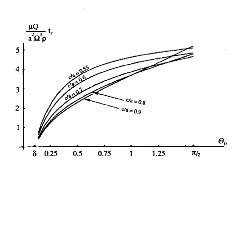
FIG. 1.: Comparison of the approximation (2.11) with the exact results for the relaxation time $\,t$. The exact calculation of $\,t\,$ (scaled by a factor of $\;\mu\,Q/a^{2}\,\Omega^{3}_{0}\,\rho\;$) was performed by combining formulae (2.9) and (2.7) for various realistic values of the parameter $\;c/a\;$. The final value of the angle $\;\theta\;$ was assumed to be $\;\delta\,=\,6^{0}\;$, while its initial value was varying from $\;\delta\;$ through $\;\pi/2\;$.

parameter $\;c/a\;$ when values of this parameter fall within the interval 0.5 - 0.9 (see Fig.1). As we can see from the plot, the dependence $\;t(\theta_{0})\;$ may be approximated, for $\;c/a\,=\,$0.5 - 0.9, by the following expression that does not bear any dependence upon $\;c/a\;$:

$$t\;\;\simeq\;\;-\;2.80\;\theta^{2}_{0}\;+\;7.84\;\theta_{0}\;-\;0.79$$ (11)

This is a rough approximation. For the above value of $\;\delta\;$, it gives an error of about 100 % for $\,\theta_{0}\,\stackrel{{\scriptstyle>}}{{\sim}}\,\delta\,$ and an error of about 10 % for $\,\theta_{0}\,>\,\pi/4\,$. Nevertheless it is more than acceptable for our purposes, for it enables one to get an idea as to what a typical value of the relaxation time could be.

III Comparison with an earlier study

We shall compare our result for the typical time of alignment with the estimate obtained in Burns & Safronov (1973):

$$t_{(B\;\&\;S)}\;\approx\;A\;\frac{\mu\;Q}{\rho\;a^{2}\;\Omega^{3}_{0}}\;\;\;,$$ (12)

the numerical factor A being about $100$ for bodies of small oblateness, and about $10$ for bodies of very irregular shapes. In astrophysics we normally encounter the case of small oblateness (except perhaps some exotic species of cosmic-dust grains, called carbon flakes), so let us assume $\;0.5\,\stackrel{{\scriptstyle<}}{{\sim}}\,c/a\,\stackrel{{\scriptstyle<}}{{\sim}}\,0.9\,$. Our formula will give:

$$t_{(our\;result)}^{c\approx a}\;\approx\;(1\;-\;2)\;\frac{\mu\;Q}{\rho\;a^{2}\;\Omega^{3}_{0}}\;\;\;\;for\;\;\;\;\theta_{0}\,\approx\,(2\;-\;3)\,\delta$$ (13)

$$t_{(our\;result)}^{c\approx a}\;\approx\;(3\;-\;4)\;\frac{\mu\;Q}{\rho\;a^{2}\;\Omega^{3}_{0}}\;\;\;\;for\;\;\;\;\theta_{0}\,\approx\,\pi/4$$ (14)

$$t_{(our\;result)}^{c\approx a}\;\approx\;(4\;-\;5)\;\frac{\mu\;Q}{\rho\;a^{2}\;\Omega^{3}_{0}}\;\;\;\;for\;\;\;\;\theta_{0}\,\stackrel{{\scriptstyle<}}{{\sim}}\,\pi/2$$ (15)

while the aforequoted formula of Burns and Safronov will read:

$$t_{(B\;\&\;S)}^{c\approx a}\;\approx\;100\;\frac{\mu\;Q}{\rho\;a^{2}\;\Omega^{3}_{0}}\;\;\;.$$ (16)

We see that in the preceding study the relaxation time was overestimated, for small initial angles, by two orders. In other words, the effectiveness of the inelastic-relaxation process was underestimated by two orders. Even when the initial angle is not too small ($\;\theta_{0}\;\sim\;\pi/4\;$), the underestimation will be by a factor of 30 or so. The three main reasons for this underestimate are the following. First, it is the contribution of the double-frequency mode missing in (Burns & Safronov 1973). In the sum $\;(63(c/a)^{4}\,\cot^{2}\theta+20)\;$ emerging in formula (7), the term $\;63(c/a)^{4}\,\cot^{2}\theta\;$ appears due to the principal mode, while the term $\;20\;$ appears due to the double-frequency mode. Thence, in the case of $\;c\;$ close to $\;a\;$ the double-frequency mode will give (after integration over $\theta$) a considerable input, while for $\;c\ll a\;$ (which is not a likely case for asteroids and comets, but may happen for cosmic dust) it provides an overwhelming contribution to the entire effect. The only case when the contribution of the second mode is irrelevant is the case of a small initial angle $\;\theta_{0}\;$. But in this case there exists another simple reason for (12) to give a large error compared to our analysis: (12) simply ignores any dependence upon the initial angle, and this is why it gives too long times for small angles. The third source of error in (12) is an assumption, accepted by Burns and Safronov, that the energy dissipation in the case of small oblateness is predominantly due to the bulge flexing. It seems that this simplifying assumption does not work well.

IV Dynamics of Prolate Bodies

At first glance, the dynamics of a freely-spinning prolate body obeys the same principles as the dynamics of an oblate one: the axis of maximum inertia will tend to align itself parallel to the angular momentum. If we model a prolate body with a symmetric top, it will be once again convenient to choose it be a prism of dimensions $\;2a\times 2a\times 2c\;$, though this time half-size $\,c\,$ is larger than $\,a\,$, and thereby $\;I_{3}\;=\;I_{2}\;>\;I_{1}\;$. Then all our calculations formally remain in force, except that the right-hand side in (A19) changes its sign, provided we keep the notation $\theta$ for the angle between $\;\mathbf{J}\;$ and the body-frame axis 3 (parallel to dimension $\;2c\;$). This brings an illusion that axis 3 tends to stand orthogonal to $\mathbf{J}$, which at first glance appears natural since axis 3 is now not the maximum-inertia but the minimum-inertia axis.

Unfortunately, this extrapolation of the oblate-body description to a prolate-body case is of absolutely no practical relevance. The problem is that an arbitrarily small difference between $\;I_{3}\;$ and $\;I_{2}\;$ will entail an entirely new character of precession (Synge & Griffith 1959). For the first time this topic, in the context of asteroid and comet precession, was addressed by Black et al (1999). We are planning to dwell on the subject comprehensively in our next article.

V Numbers

Values of the involved parameters may depend both upon the temperature of the body and the wobble frequency. Evidently, the temperature-, pressure- and frequency-caused variations of the density $\;\rho\;$ are tiny and may be neglected. This way, we can use the (static) densities appropriate to the room temperature and pressure: $\rho^{(silicate)}\;\approx\;2500\;kg\;m^{-3}\,$ and $\rho^{(carbon)}\;\approx\;2000\;kg\;m^{-3}$.

As for the adiabatic shear modulus $\;\mu\;$, tables of physical quantities would provide its values at room temperature and atmospheric pressure, and for quasistatic regimes solely. As for the possible frequency-related effects in materials (the so-called ultrasonic attenuation), these become noticable only at frequencies higher than $\;10^{8}\;Hz\;$ (see section 17.7 in Nowick and Berry 1972). Another fortunate circumstance is that the pressure-dependence of the elastic moduli is known to be weak (Ahrens 1995). Besides, the elastic moduli of solids are known to be insensitive to temperature variations, as long as these variations are far enough from the melting point. The value of $\;\mu\;$ may increase by several percent when the temperature drops from room temperature to $\;10\,K\;$. Dislocations don’t affect the elastic moduli either. Solute elements have very little effect on moduli in quantities up to a few percent. Besides, the moduli vary linearly with substitutional impurities (in which the atoms of the impurity replace those of the hosts). However hydrogen is not like that: it enters the interstices between the atoms of the host, and has marginal effect on the modulus. As for the role of the possible porosity, the elastic moduli scale as the square of the relative density. For porosities up to about $20\;\%~{}\,$, this is not of much relevance for our estimates.

According to Ryan and Blevins (1987), for both carbonaceous and silicate rocks one may take the shear-modulus value $\mu\;\approx\;10^{10}\;Pa\;\;$. For the dirty ice Peale and Lissauer (1989) suggest, for Halley’s comet, $\;\mu\;\approx\;10^{10}\;dyne/cm^{2}\;=\;10^{9}\;Pa\;$ while $\;Q\;<\;100\;$.

A proper choice of the values of the $\;Q-$factor for asteroids is to be the most problematic subject. As well known from seismology, the $\;Q-$factor bears a pronounced dependence upon: the chemical composition, graining, frequency, temperature, and confining pressure. It is, above all, a steep function of the humidity which presumably affects the interaction between grains. The $\;Q-$factor is less sensitive to the porosity (unless the latter is very high); but it greatly depends upon the amount and structure of cracks, and generally upon the mechanical nature of the aggregate. Whether comets and asteroids are loose aggregates or solid chunks remains unknown. The currently available experimental data are controversial. On the one hand, it is a well-established fact that comets sometimes get shattered by tidal forces. Namely, Shoemaker-Levy 9 broke into 21 pieces on the perijove preceding the impact (Marsden 1993). It seems that at least some comets are loosely connected aggregates, though we are unsure if all comets are like this.

As for the asteroids, the question is yet open, and the low density of asteroid 253 Mathilde (about 1.2 $\;g/cm^{3}$) may be either interpreted in terms of the rubble-pile hypothesis (Harris 1998), or put down to Mathilde being perhaps mineralogically akin to low-density carbonaceous chondrites, or be explained by a very high porosity. In our opinion, the sharply-defined craters on the surfaces of some asteroids witness against the application of the rubble-pile hypothesis to asteroids . And of course, we should mention here Vesta as a reliable example of an asteroid being a solid body of a structure common for terrestial planets: Hubble images of Vesta have revealed basaltic regions of solidified lava flows, as well as a deep impact basin exposing solidified mantle. Thus we would say that at least some asteroids are well connected solid chunks, though we are uncertain whether this is true for all asteroids.

In the sequel, hence, we shall assume that the body is not a loosely connected aggregare but a solid rock (possibly porous but nevertheless solid and well-connected), and shall try to employ some knowledge available on attenuation in the terrestial and lunar crusts.

We are in need of the values of the quality factors for silicate and carbonateous rocks. We need these at the temperatures from several K to dozens of K, , zero confining pressure, frequencies appropriate to asteroid precession ($10^{-6}\;-\;10^{-4}\;Hz$), and (presumably!) complete lack of moisture.

Much data on the behaviour of $\;Q-$factors is presented in the seismological literature. Almost all of these measurements have been made under high temperatures (from several hundred up to 1500 Celsius), high confining pressures (up to dozens of MPa), and unavoidably in the presence of humidity. Moreover, the frequencies were typically within the range from dozens of $kHz$ up to several $MHz$. Only a very limited number of measurements have been performed at room pressure and temperature, while no experiments at all have been made thus far with rocks at low temperatures (dozens of $\;K\;$). The information about the role of humidity is extremely limited. Worst of all, only a few experiments were made with rocks at the lowest seismological frequences ($10^{-3}\;-\;10^{-1}\;Hz$), and none at frequencies between $\;10^{-6}\;$ and $\;10^{-2}\;Hz$, though some indirectly achieved data are available (see Burns 1977, Burns 1986, Lambeck 1980, and references therein).

It was shown by Tittman et al. (1976) that the $\;Q-$factor of about $\;60\;$ measured under ambient conditions on an as-received lunar basalt was progressively increased ultimately to about $\;3300\;$ as a result of outgassing under hard vacuum. The latter number will be our starting point. The measurements were performed by Tittman et al. at $\;20\;kHz\;$ frequency, room temperature and no confining pressure. How might we estimate the values of $\;Q\;$ for the lunar basalt, appropriate to the lowest frequencies and temperatures?

As for the frequency-dependence, it is a long-established fact (e.g., Jackson 1986, Karato 1998) that $\;\;Q\;\sim\omega^{\alpha}\;$ with $\;\alpha\;$ around 0.25. This dependence reliably holds for all rocks within a remarkably broad band of frequencies: from hundreds of $\;kHz\;$ down to $\;10^{-1}Hz$. Very limited experimental data are avaliable for frequencies down to $\;10^{-3}Hz$, and none below this threshold. Keep in mind that $\;\alpha\;$ being close to 0.25 holds well only at temperatures of several hundred Celsius and higher, while at lower temperatures $\;\alpha\;$ typically decreases to 0.1 and less.

As regards the temperature-dependence, there is no consensus on this point in the geological literature. Some authors (Jackson 1986) use a simple rule:

$$\;Q\;\sim\;\omega^{\alpha}\;\exp(A^{*}/RT)\;\;\;,$$ (17)

$\;A^{*}\;$ being the apparent activation energy. A more refined treatment takes into account the interconnection between the frequency- and temperature-dependences. Briefly speaking, since the quality factor is dimensionless, it must retain this property despite the exponential frequency-dependence. This may be achieved only in the case that $\;Q\;$ is a function not of the frequency per se but of a dimensionless product of the frequency by the typical time of defect displacement. The latter exponentially depends upon the activation energy, so that the resulting dependence will read:

$$\;Q\;\sim\;\left[\omega\;\exp(A^{*}/RT)\right]^{\alpha}\;\;\;,$$ (18)

where $\;A^{*}\;$ may vary from 150 - 200 $\;kJ/mol\;$ (for dunite and polycristalline forsterite) up to 450 $\;kJ/mol\;$ (for olivine). This interconnection between the frequency- and temperature-dependences tells us that whenever we lack a pronounced frequency-dependence, the temperature-dependence is absent too. It is known, for example (Brennan 1981) that at room temperature and pressure, at low frequencies ($10^{-3}\;-\;1\;Hz$) the shear $\;Q-$factor is almost frequency-independent for granites and (except some specific peak of attenuation, that makes $Q$ increase twice) for basalts. It means that within this range of frequencies $\;\alpha\;$ is small (like 0.1, or so), and $\;Q\;$ may be assumed almost temperature-independent too.

Presumably, the shear Q-factor, reaching several thousand at $\;20\;kHz\;$, descends, in accordance with (18), to several hundred when the frequency decreases to several $\;Hz$. Within this band of frequencies, we should use the power $\;\alpha\,\approx\,0.25\;$, as well known from seismology. When we go to lower frequencies (from several $\;Hz$ to the desirable $10^{-6}\;-\;10^{-4}\;Hz$), the Q-factor will descend at a slower pace: it will obey (18) with $\;\alpha\,<\,0.1\;$. Low values of $\;\alpha\;$ at low frequencies are mentioned in Lambeck (1980) and in Lambeck (1988). The book by Lambeck containes much material on the $Q$-factor of the Earth. Unfortunately, we cannot employ the numbers that he suggests, because in his book the quality factor is defined for the Earth as a whole. Physically, there is a considerable difference between the $Q$-factors emerging in different circumstances, like for example, between the effective tidal $Q$-factor and the $Q$-factor of the Chandler wobble). In regard to the latter, Lambeck (1988) refers, on page 552, to Okubo (1982) who suggested that for the Chandler wobble $\;50\,<\,Q\,<\,100\;$. Once again, this is a value for the Earth as a whole, with its viscous layers, etc. We cannot afford using these numbers for a fully solid asteroid.

Brennan (1981) suggests for the shear $\;Q-$factor the following values: $Q^{(granite)}_{(shear)}\;\approx\;250\;$, $\;Q^{(basalt)}_{(shear)}\;\approx\;500\;$. It would be tempting to borrow these values, if not for one circumstance: as is well known, absorption of only several monolayers of a saturant may dramatically decrease the quality factor. We have already mentioned this in respect to moisture, but the fact is that this holds also for some other saturants. Since the asteroid material may be well saturated with hydrogen (and possibly with some other gases), its $\,Q$-factor may be much affected.

It may be good to perform experiments, both on carbonaceous and silicaceous rocks, at low frequencies and temperatures, and with a variety of combinations of the possible saturants. These experiments should give us the values for both shear and bulk quality factors. The current lack of experimental data gives us no choice but to start with the value 3300 obtained by Tittman for thoroughly degassed basalts, and then to use formula (18). This will give us, at $\;T\,=\,20\;K\;$ and $\;\omega\,=\,10^{-5}\;Hz\;$:

$$Q^{(basalt)}_{(shear)}\;\approx\;150$$ (19)

This value of the shear $Q$-factor for granites and basalts differs from the one chosen in Burns and Safronov (1979) only by a factor of 2. For carbonaceous materials $\;Q\;$ must be surely much less than that of silicates, due to weaker chemical bonds. So for carbonaceous rocks we shall choose the following upper boundary:

$$Q^{(carb)}\;<\;100\;\;\;,$$ (20)

though this boundary is somewhat arbitrary, and is probably still too high.

Terrestial geophysics has not yet given us a reliable handle on the acoustic properties of asteroids and comets, though the necessary quality factors can be obtained by a modification of the existing testing technique. Namely, the frequencies must be within the interval $\;10^{-6}\;-\;10^{-4}\;Hz$, the temperature must be from about $\;K\;$ to dozens of $\;K\;$. The specimens must be well outgassed and the measurements must be performed under a high vacuum that would mimic the real interplanetary environment. It would be most important to study specimens exposed to a variety of saturants (hydrogen, first of all). The specimens must include both silicate and carbonaceous rocks, and artificially or naturally prepared samples of dirty ice.

Twenty two years ago J.A. Burns (1977) wrote: “Further experimental and theoretical work for real materials is sorely needed if we are to ever trace the history of the natural satellites.” This plea is even more relevant today, and the ramifications of such work will nowadays be even broader: these studies are to become our key not only to satellite but also to asteroid studies.

VI Particular example: Asteroid 4179 Toutatis

The asteroid 4179 Toutatis is a slowly rotating body of size about 2 $km$, that was “imaged” in radar by Ostro et al. (1993), (1995), (1999), Hudson and Ostro 1995, Scheeres et al. 1998. It is of S-type, analogous to stony irons or ordinary chondrites but certainly not to carbonaceous chondrites (Ostro et al. 1999). It has a rotation period $\;\tau\;=\;7.5\;days\;$ (so that $\Omega_{0}\;=\;2\pi/\tau\;\approx\;9.7\times 10^{-6}\;Hz$).

Our analysis was aimed at oblate bodies and, rigorously speaking, it is unapplicable to prolate or triaxial rotators. Still, while a similar study for triaxial rotators in on the way, let us try to apply our formulae, as a zeroth approximation, to Toutatis. Suppose that some tidal interaction has forced this asteroid to precess with a small precession-cone half angle $\;\theta_{0}\;$. Let it be, for example, twice or thrice the minimally recognisable half-angle: $\;\theta_{0}\;=\;(2\,-\,3)\,\delta\;\sim\;12^{o}\;$. Then Fig.1 (or our formula (14) based on it) will give, for $\;Q\,=\,150\;$, $\;\mu\,=\,10^{11}\,dyne/cm^{2}\,=\,10^{10}\;Pa\;$, and $\;\rho\,=\,2000\;kg/m^{3}$, $\;c/a\,\stackrel{{\scriptstyle>}}{{\sim}}\,1/2\;$:

$$t\;\stackrel{{\scriptstyle<}}{{\sim}}\;2.5\;\frac{\mu\;Q}{\rho\,a^{2}\,\Omega^{3}_{0}}\;=\;0.5\;\times 10^{18}\;s\;\approx\;1.6\;\times\;10^{10}\;years$$ (21)

which is 800 times less than the estimate that would come from Burns & Safronov’s (1973) treatment. Factor 800 emerges, first, due to the difference by a factor of 40 between our formula (21) and Burns & Safronov’s formula (16); and second, due to the difference in choice of the quality-factor and shear-modulus values. Our choice is: $\;\mu Q\;=\;1.5\;\times\;10^{13}\;dyne/cm^{2}\;=\;1.5\;\times\;10^{12}\;Pa\;$, while Burns & Safronov suggested $\;\mu Q\;=\;3\;\times\;10^{14}\;dyne/cm^{2}\;=\;3\;\times\;10^{13}\;Pa\;$. We suggest values lower than in Burns & Safronov (1973) for the reasons explained above.

Harris (1994) goes even further: he suggests to use data measured for Phobos: $\;\mu Q\;=\;5\;\times\;10^{12}\;dyne/cm^{2}\;=\;5\;\times\;10^{11}\;Pa\;$ which is almost two orders of magnitude less than that in Burns & Safronov (1979). Therefore if we adopt the values proposed by Harris (1994), our estimate (21) will be further decreased by 3 times, and will equal to $\;5\;\times\;10^{9}\;years\;$, which is $\;10^{3}\;$ times less than the result that would follow from Burns & Safronov’s treatment.

Even though Harris chose a lower value for $\mu Q$ than we did, our calculation will give a lower value for the relaxation time, due to the difference in numerical factors in our formula (14) and Burns & Safronov’s formula (16). (Actually, this difference is even larger than it should be, because Harris, applying Burns & Safronov’s formula, took the overall numerical factor to be not 10 but 30.) This would mean that the number of asteroids that are suspected of tumbling (see Fig. 1 in Harris (1994)) should be decreased.

How certain is this conclusion? It follows from our discussion in the previous section that at least for solid asteroids the $\mu Q$ factor obtained for Phobos in Yoder (1982) may be an underestimate. Observations of asteroid precession should provide us with insight into their mechanical properties. The comparison of these with the properties of laboratory-studied materials should provide us with more understanding of the composition and inner structure of asteroids.

While studying wobbling, it is important to bear in mind two points. First of all, nutations at small angle can proceed for much longer times than we estimated above. This is the consequence of the “slow finish” condition that we discussed in section III. With the improvement of the radar measurements, we expect to detect more asteroids wobbling at small angles. Therefore high-accuracy imaging of asteroids may reveal nutations above the upper curve in Fig. 1 in Harris (1994). Second, large-amplitude or/and rapid tumbling may be suppressed quicker than we estimated as the strains become nonlinear and the dissipation increases.

VII Conclusions

1. The dissipation at the double frequency of precession makes an importantm, sometimes decisive, contribution into the process of inelastic relaxation.

2. Small-amplitude wobbling can proceed for long periods of time, while the large-amplitude precession gets damped to smaller amplitudes much faster. This is a consequence of the dependence of the relaxation rate upon the angle of precession. In reality, the finite resolution of radar-generated images makes us take into consideration only wobble with precession-cone half angles no less than about $\;5\,-\,6^{o}\;$. (Though observations made by spacecrafts will, hopefully, improve the resolution up to one degree or so.)

3. Neglection of the above two circumstances, along with acceptance of an assumption (unjustified, in our opinion) that the tidal-bulge flexing plays a decisive role in the inelastic relaxation, lead our predecessors to a great underestimate of the effectiveness of the inelastic dissipation mechanism. (By two orders, for small initial angles, and by a factor of 20 - 30 for large angles.)

4. Solid asteroids are likely to have $Q-$factors about one hundred, or possibly even less, but further laboratory research is required. Earth seismological data may poorly represent acoustic properties of asteroids and comets as even a tiny trace of moisture (several monolayers) substantially alters the quality factor. Laboratory data on $\;10^{-6}\;-\;10^{-4}\;Hz\;$ oscillations of de-moisturised silicate and carbonaceous rocks at temperatures within the range from several $\;K\;$ to several dozens $\;K\;$ are badly needed.

5. Potentially, wobbling may provide valuable information on the composition and structure of asteroids, and on their recent history of external impacts.

6. Since the inelastic dissipation turns out to be a far more effective process than believed previously, the number of asteroids expected to wobble with a large angle of the precession cone is expected to be lower (than the predictions made in (Harris 1994).)

Acknowledgements

The authors are grateful to Eric Heller for encouragement, and to Alan Harris and Steven Ostro for stimulating discussions that helped us to considerably improve the article. M.E. would like to acknowledge very useful information on the properties of materials, provided by Michael Aziz and Michael Ashby, and a consultation on radar accuracy, by Scott Hudson. A.L. acknowledges discussions with Bruce Draine, and a couple of suggestions by Scott Tremaine. The work of A.L. was supported by NASA grant NAG5-2858. This paper would never have been completed without a comprehensive tutorial on the Q-factor, so kindly offered to us by Shun-ichiro Karato: his consultation gave a second breath to our project.

A Alignment of the maximal-inertia axis towards the angular-momentum vector

If we model the freely rotating oblate body by a prism of sizes $2a\times 2a\times 2c$, ($c<a$) and density $\;\rho\;$, the time-dependent stresses will read (Lazarian and Efroimsky 1998):

$$\sigma_{xx}=\frac{\rho\Omega_{\perp}^{2}}{4}(x^{2}-a^{2})\;\cos 2{\omega}t\;\;,\;\;\;\sigma_{yy}=-\frac{\rho\Omega_{\perp}^{2}}{4}(y^{2}-a^{2})\;\cos 2{\omega}t\;\;,\;\;\;\sigma_{zz}=0$$ (A1)

$$\sigma_{xy}\;\;=\;\;\frac{\rho}{4}\;\Omega_{\perp}^{2}\;(x^{2}\;\;+\;\;y^{2}\;\;-\;\;2a^{2})\;\;\sin\;2{\omega}t\;\;\;,$$ (A2)

$$\sigma_{xz}\;\;=\;\;\frac{\rho}{2}\;{\Omega_{\perp}}\;{\Omega_{3}}\;\left[\;h\;(z^{2}\;-\;c^{2})\;\;+\;\;(2\;-\;h)\;(x^{2}\;-\;a^{2})\;\right]\;\;\cos\;{\omega}t\;\;\;,$$ (A3)

$$\sigma_{yz}\;\;=\;\;\frac{\rho}{2}\;{\Omega_{\perp}}\;{\Omega_{3}}\;\left[\;h\;(z^{2}\;-\;c^{2})\;\;+\;\;(2\;-\;h)\;(y^{2}\;-\;a^{2})\;\right]\;\;\sin\;{\omega}t\;\;\;.$$ (A4)

As expected, not only the principal frequency but also the second mode shows up in $\sigma_{ij}$.

The moment of inertia $\;I_{3}\;$ and the parameter $\;h\;$ read:

$$I_{3}\;=\;\frac{16}{3}\;\rho\;a^{4}\;c\;\;\;\;\;,\;\;\;\;\;\;\;\;h\;\;\equiv\;\;\frac{I_{3}}{I}\;\;=\;\;\frac{2}{1\;+\;(c/a)^{2}}\;\;\;\;\;.\;\;\;$$ (A5)

According to (6),

$$\Omega_{3}\;\;=\;\;\Omega_{0}\;\cos\theta\;\;\;\;\;,\;\;\;\;\;\;\;\;\;\;\;\;\Omega_{\perp}\;\;=\;\;\Omega_{0}\;h\;\sin\theta\;\;\;,$$ (A6)

$\Omega_{0}\equiv J/I_{3}$ being the typical angular velocity of a body. We shall compute the strain tensor in order to estimate the maximal elastic energy $\,W\,$ stored in the body. Then, we shall estimate the dissipation rate as $\,-\omega W/Q\,$, $\;Q\;$ being the quality factor of the material.

The kinetic energy of an oblate spinning body reads, according to (1), (2), and (6):

$$E_{rot}\;=\;\frac{1}{2}\;[I\;\Omega_{\perp}^{2}\;+\;I_{3}\;{\Omega_{3}}^{2}]\;=\;\frac{1}{2}\;\;\left[\;\frac{1}{I}\;\;\sin^{2}\;\theta\;\;+\;\;\frac{1}{I_{3}}\;\;\cos^{2}\;\theta\;\right]\;J^{2}$$ (A7)

so that

$$\frac{dE_{rot}}{d\theta}\;\;=\;\;\frac{J^{2}}{I_{3}}\;(h\;-\;1)\;\;\sin\;\theta\;\;\cos\;\theta\;\;=\;\;\omega\;J\;\;\sin\;\theta\;\;\;.$$ (A8)

The rotational energy changes via the inelastic dissipation:

$$\dot{E}_{rot}\;=\;\dot{W}\;\;\;,$$ (A9)

$\;W\;$ standing for the elastic energy of the body. Then the rate of alignment is:

$$\frac{d\theta}{dt}\;=\;\left(\frac{dE_{rot}}{d\theta}\right)^{-1}\frac{dE_{rot}}{dt}\;=\;\left(\omega\;J\;\;\sin\;\theta\right)^{-1}\;\dot{W}$$ (A10)

where

$$\dot{W}\;=\;\dot{W^{({\omega})}}\;+\;\dot{W^{(2{\omega})}}\;=\;-\;\omega\;\frac{W_{0}^{({\omega})}}{Q^{({\omega})}}\;-\;2\;\omega\;\frac{W_{0}^{({2\omega})}}{Q^{({2\omega})}}\;\approx\;\frac{2\,\omega}{Q}\;\left\{W^{({\omega})}\;+\;2W^{({2\omega})}\right\}\;\;\;,$$ (A11)

the quality factor being almost frequency-independent. In reality, it certainly does depend upon $\omega$, but the dependence is very smooth and may be neglected for frequencies differing by a factor of two. (It should be taken into account within frequency spans of several orders.) In (A11) $W_{0}^{\omega}\,,\;W_{0}^{2\omega}$ denote the amplitudes of the elastic energies associated with vibrations at the modes $\omega$ and $2\omega$, while $W^{\omega}\,=\,2\,W_{0}^{\omega}\,$ and $\,W^{2\omega}\,=\,2\,W_{0}^{2\omega}$ stand for the averages. In our preceding publication (Lazarian and Efroimsky 1998) we missed the coefficient 2 between $W_{0}^{(...)}$ and $W^{(...)}$.

Now the question is: how to calculate $\;W^{({\omega})}\;+\;2W^{({2\omega})}\;$? At low temperatures the bodies manifest, for small displacements (like, say, sound) no viscosity: $\;\;\omega\eta\,\sim\,\omega\zeta\;\ll\;\mu\,\sim\,K\;$. Hence the stress tensor will be approximated, to a high accuracy, by its elastic part:

$$\epsilon_{ij}\;\;=\;\;\delta_{ij}\;\;\frac{Tr\;\sigma}{9\;K}\;\;+\;\;\left(\;\sigma_{\it{ij}}\;\;-\;\;\frac{1}{3}\;\;\delta_{ij}\;\;Tr\;\sigma\right)\;\frac{1}{2\;\mu}\;\;\;~{}~{}~{},$$ (A12)

$K\,$ and $\,\mu\,$ being the bulk and shear moduli. The elastic energy stored in a unit volume is

$$dW/dV\;=\;\frac{1}{2}\;\epsilon_{ij}\;\sigma_{ij}\;=\;\frac{1}{4}\;\left\{\left(\frac{2\;\mu}{9\;K}\;-\;\frac{1}{3}\right)\,\left(Tr\;\sigma\right)^{2}\;+\;\sigma_{ij}\,\sigma_{ij}\right\}\;\;\;\;.$$ (A13)

Anticipating different rates of dissipation in the two modes, we split $dW/dV$ into parts:

$$dW/dV\;=\;dW^{(\omega)}/dV\;+\;dW^{(2\omega)}/dV$$ (A14)

According to (A11), what we need is the sum

$$W^{({\omega})}\;+\;2W^{({2\omega})}\;=\;\int^{a}_{-a}\,dx\;\int^{a}_{-a}\,dy\;\int^{c}_{-c}\,dz\;\left\{dW^{({\omega})}/dV\;+\;2\;dW^{({2\omega})}/dV\right\}$$ (A15)

To compute this sum, one has to plug the expressions for stresses (A1) - (A4) into (A13), then to split the result in accordance with (A14), and to build up the sum under the integral in (A15). These calculations (presented in (Lazarian and Efroimsky 1999)) yield:

$$W^{({\omega})}\,+\,2\,W^{({2\omega})}\,=\,\frac{3^{2}\,2^{-6}\,(63\,(c/a)^{4}\,\tan^{-2}\theta\,+\,20)}{\mu}\;\frac{a^{-2}\;c^{-1}}{\left[1+(c/a)^{2}\right]^{4}}\;\left(\frac{I_{3}\,\Omega_{0}^{2}}{2}\right)^{2}\;\sin^{4}\theta\;\;\;$$ (A16)

where $\;\Omega_{0}\,\equiv\,J/I_{3}\;$ is a typical angular velocity. Eventually, (A10), (A11) and (A16) will yield:

$$d\theta/dt\;=\;-\;\frac{3^{2}\;2^{-6}\;(63\;(c/a)^{4}\;\tan^{-2}\theta\;+\;20)}{\mu\;Q\;J}\;\frac{a^{-2}\;c^{-1}}{\left[1+(c/a)^{2}\right]^{4}}\;\left(\frac{I_{3}\;\Omega_{0}^{2}}{2}\right)^{2}\;\sin^{3}\theta$$ (A17)

According to (A5) and (8),

$$\frac{1}{J}\;\left(\frac{I_{3}\,\Omega^{2}_{0}}{2}\right)^{2}\;=\;\frac{4}{3}\;\Omega_{0}^{3}\;\rho\;a^{4}\;c$$ (A18)

Substitution of the latter in the former gives the final expression for the alignment rate:

$$d\theta/dt\;=\;-\;\frac{3}{2^{4}}\;\sin^{3}\theta\;\;\frac{63\;(c/a)^{4}\;\cot^{2}\theta\;+\;20}{[1+(c/a)^{2}]^{4}}\;\;\frac{a^{2}\;\Omega^{3}_{0}\;\rho}{\mu\;Q}$$ (A19)

REFERENCES

- [1] Ahrens, T.J. 1995 Ed., Mineral Physics & Crystallography. A Handbook of Physical Constants. American Geophysical Union, Washington DC
- [2] Black, G.J, P.D.Nicholson, W.Bottke, Joseph A.Burns, & Allan W. Harris 1999, ”On a Possible Rotation State of (433) Eros” - Icarus, Vol. 140, p. 239
- [3] Brennan, B.J. 1981, in: Anelasticity in the Earth (F.D.Stacey, M.S.Paterson and A.Nicolas, Editors), Geodynamics Series 4, AGU, Washington.
- [4] Burns, J. A. and Safronov, V.S. 1973, MNRAS, 165, p. 403
- [5] Burns, J. A. 1977, in: Planetary Satellites, J.A.Burns, Ed., University of Arizona Press, Tucson
- [6] Burns, Joseph A. 1986, in: Satellites, J.A.Burns, Ed., University of Arizona Press, Tucson
- [7] Clark V.A., B.R.Tittman and T.W. Spencer 1980, J. Geophys. Res., 85, p. 5190
- [8] Fowles, Grant R., and George L. Cassiday 1986 Analytical Mechanics. Harcourt Brace & Co, Orlando, FL
- [9] Goldreich, Peter, & Steven Soter 1965, Icarus, Vol. 5, p. 375
- [10] Harris, Alan W. 1994, Icarus, 107, p. 209
- [11] Harris, Alan W. 1998, Nature, Vol. 393, p. 418
- [12] Hudson, R.S., and S. J. Ostro 1995, Science 270, 84-86
- [13] Jackson, Ian 1986, in: Mineral and Rock Deformation. Laboratory Studies, American Geophysical Union, Washington DC
- [14] Karato, Shun-ichiro 1998, Pure and Applied Geophysics, in press
- [15] Knopoff, L. 1963, Reviews of Geophysics, Vol.2, p. 625
- [16] Lambeck, Kurt 1980 The Earth’s Variable Rotation: Geophysical Causes and Consequencies, Cambridge University Press, Cambridge, U.K.
- [17] Lambeck, Kurt 1988 Geophysical Geodesy, Oxford University Press, Oxford & NY
- [18] Landau, L.D. & Lifshitz, E.M. 1976 Mechanics, Pergamon Press, NY
- [19] Lazarian, A. & Draine, B.T., 1997, ApJ, 487, 248
- [20] Lazarian, A. and Efroimsky, M. 1999, MNRAS, Vol. 303, pp. 673 - 684
- [21] Marsden, B. & S. Nakano 1993, IAU Circ. No 5800, 22 May 1993; Marsden, B. & A. Carusi 1993, IAU Circ. No 5801, 22 May 1993.
- [22] Melosh, H.H. and P. Schenk 1993, Nature, Vol. 365, p. 731
- [23] Nowick, A.S. and Berry, D.S. 1972 Anelastic Relaxation in Crystalline Solids, Academic Press, NY
- [24] Okubo, S. 1982, Geophys.J., Vol. 71, p. 647
- [25] Ostro, S.J., Jurgens, R.F., Rosema, K.D., Whinkler, R., Howard, D., Rose, R., Slade, D.K., Youmans, D.K, Cambell, D.B., Perillat, P, Chandler, J.F., Shapiro, I.I., Hudson, R.S., Palmer, P., and DePater, I., 1993, BAAS, Vol.25, p.1126
- [26] Ostro, S.J., R.S.Hudson, R.F.Jurgens, K.D.Rosema, R.Winkler, D.Howard, R.Rose, M.A.Slade, D.K.Yeomans, J.D.Giorgini, D.B.Campbell, P.Perillat, J.F.Chandler, and I.I.Shapiro, 1995, Science, Vol. 270, p.80-83
- [27] Ostro, S.J., R.S.Hudson, K.D.Rosema, J.D.Giorgini, R.F.Jurgens, D.Yeomans, P.W.Chodas, R.Winkler, R.Rose, D.Choate, R.A.Cormier, D.Kelley, R.Littlefair, L.A.M.Benner, M.L.Thomas, and M.A.Slade 1999, Icarus, Vol. 137, p. 122-139
- [28] Ostro, S.J., Petr Pravec, Lance A. M. Benner, R. Scott Hudson, Lenka Sarounova, Michael D. Hicks, David L. Rabinowitz, James V. Scotti, David J. Tholen, Marek Wolf, Raymond F. Jurgens, Michael L. Thomas, Jon D. Giorgini, Paul W. Chodas, Donald K. Yeomans, Randy Rose, Robert Frye, Keith D. Rosema, Ron Winkler, and Martin A. Slade, 1999, Science Magazine, Vol. 285, p. 557 - 559
- [29] Peale, S. J., and J. J. Lissauer, 1989, Rotation of Halley’s Comet. Icarus, Vol. 79, p. 396-430.
- [30] Purcell, E.M. 1979, Astrophysical Journal, Vol. 231, p.404
- [31] Ryan, M.P. and Blevins, J.Y.K. 1987 U.S. Geological Survey Bulletin, Vol.1764, p.1
- [32] Sekanina Z. 1982, in: Comets, ed. by L.L.Wilkening, University of Arizona Press, Tuscon, pp. 251 - 287
- [33] Scheeres, D.J., S.J.Ostro, R.S.Hudson, S.Suzuki, and E. de Jong 1998, Icarus, Vol. 132, p. 53-79
- [34] Spencer, J.W. 1981, J. Geophys. Res., 86, p. 1803.
- [35] Synge, J.L. & B.A. Griffith 1959 Principles of Mechanics, Chapter 14, McGraw-Hill, NY
- [36] Tittman, B.R., L. Ahlberg, and J. M. Curnow, 1976, Proc. 7-th Lunar Sci. Conf., 3123-3132
- [37] Tschoegl, N.W. 1989 The Phenomenological Theory of Linear Viscoelastic Behaviour. An Introduction. Springer-Verlag, NY
- [38] Yoder, C.F. 1982, Icarus, Vol. 49, p. 327