Stability of disk galaxies in the modified dynamics

Abstract

General analytic arguments lead us to expect that in the modified dynamics (MOND) self-gravitating disks are more stable than their like in Newtonian dynamics. We study this question numerically, using a particle-mesh code based on a multi-grid solver for the (nonlinear) MOND field equation. We start with equilibrium distribution functions for MOND disk models having a smoothly truncated, exponential surface-density profiles and a constant Toomre $Q$ parameter. We find that, indeed, disks of a given “temperature” are locally more stable in MOND than in Newtonian dynamics. As regards global instability to bar formation, we find that as the mean acceleration in the disk is lowered, the stability of the disk is increased as we cross from the Newtonian to the MOND regime. The degree of stability levels off deep in the MOND regime, as expected from scaling laws in MOND. For the disk model we use, this maximum degree of stability is similar to the one imparted to a Newtonian disk by a halo three times as massive at five disk scale lengths.

1 Introduction

Underlying MOND is the assumption that galaxies do not posses a significant dark halo. As pointed out by Ostriker and Peebles (1973), a massive dark halo may be an important stabilizing agent of galactic disks. It is thus interesting to compare the stability of bare disks in MOND to the stability of similar Newtonian disks with dark halos. Such considerations may also provide a MOND explanation (see Milgrom (1989)) of the revised Freeman law whereby the distribution of central surface brightnesses of galactic disks appears to be cutoff rather sharply above a certain surface brightness $B_{0}$, (see e.g. McGaugh (1996) for a recent review and references). Translating this value of $B_{0}$ into a mean surface density (for exponential disks) one obtains a limiting surface density that is nearly $\Sigma_{0}\equiv a_{0}G^{-1}$, with $a_{0}$ the acceleration constant of MOND. In MOND, disks with a mean surface density $\Sigma>>\Sigma_{0}$ have a different dynamical behavior than those with $\Sigma<\Sigma_{0}$. In particular the former are Newtonian and thus are beset by the well-known instabilities of bare Newtonian disks. The latter are more stable locally (as shown in Milgrom (1989) using perturbation theory) and, as we shall show in this work, are also more stable globally. Global added stability is also supported by preliminary N-body calculations carried out by Christodoulou (1991), and by Griv and Zhytnikov (1995). The Freeman law, which asserts that the former type of disk is rare, may result from this disparity.

Toomre showed that in Newtonian dynamics a disk is stable to all local axisymmetric disturbances at radius R if the dimensionless quantity

$$Q(R)=\frac{\sigma_{R}\kappa}{3.36G\Sigma}>1,$$ (1)

where $\sigma_{R}$ is the radial velocity dispersion, $\kappa$ is the epicycle frequency, and $\Sigma$ is the surface density. The criterion in MOND is obtained by simply replacing $G$ by $G/\mu^{+}(1+L^{+})^{1/2}$, where $\mu^{+}$ is the value of the MOND interpolating function, $\mu$, just above the disk, and $L=d\ln\mu(x)/d\ln(x)$ (Milgrom (1989)). Although Toomre’s criterion rests on local analysis, it is found empirically that the condition $Q>1$ everywhere in the disk is a necessary and sufficient condition for global axisymmetric stability. Stellar disks are always stable to local non-axisymmetric disturbances (Goldreich and Lynden-Bell (1965); Julian and Toomre (1966)). Numerical simulations have shown that stellar disks are subject to global non-axisymmetric instabilities, especially the bar instability. This result was confirmed analytically for a few models by linear, normal-mode analysis. The majority of rotationally supported, self-consistent disk models studied to date by numerical simulations and analytical global analysis are violently unstable to bar formation. However, these simulations do not reveal the mechanism of the instability nor suggest a way to avoid it. Toomre (1981) suggested a mechanism for the bar instability based on what he named swing amplification.

Even the Newtonian-plus-dark-matter case the stability problem is anything but resolved. So, we shall not focus our work on testing for absolute stability in MOND. Instead we perform a comparative study between the added stability given to the disk by MOND, and that given by a dark halo. In particular we shall ask to what extent can MOND replace the halo’s contribution to the stability of disk galaxies.

Even for Newtonian gravity one lacks simple analytic equilibrium solutions of the collisionless Boltzmann equation for a thin disk. Some of the equilibrium models studied to date are the Isochrone by Kalnajs (1978), Kuzmin-Toomre (Sellwood (1986); Hunter (1992)), and the Sawamura disks (Sawamura (1983)). The extent to which the bar instability and others depend on the specific properties of these models is unknown. The situation for MOND is even more difficult since we have no analogous analytical models. The analytical methods used in Kalnajs (1972) and Kalnajs (1977) for linear, normal-mode analysis are very cumbersome and give no physical insight into the nature of the instability. A simpler way to get the unstable modes is through N-body simulations. We have developed a three-dimensional, N-body code and potential solver for the nonlinear MOND problem, in which the potential is determined from the equation proposed by Bekenstein and Milgrom (1984).

2 Description of the MOND potential solver

Bekenstein and Milgrom (1984) have formulated a non-relativistic Lagrangian theory for MOND, in which the acceleration field ${\bf g}$ produced by a mass distribution $\rho$ is derived from a potential $\phi$ (${\bf g}=-\vec{\nabla}\phi$) satisfying the equation

$$\vec{\nabla}\cdot[\mu(|\vec{\nabla}\phi|/a_{0})\vec{\nabla}\phi]=4\pi G\rho$$ (2)

instead of the usual Poisson equation $\vec{\nabla}\cdot\vec{\nabla}\phi=4\pi G\rho$, where $\mu(x)\approx x$ for $x\ll 1$, and $\mu(x)\approx 1$ for $x\gg 1$, and $a_{0}$ is the acceleration constant of MOND. The form $\mu(x)=x/\sqrt{1+x^{2}}$ has been used in all rotation curve analyses and we also use it here. A solution to the field equation exists and is unique in a domain $D$ in which $\rho({\bf r})$ is given and on the boundary of which $\phi$, or $\mu(|\vec{\nabla}\phi|/a_{0})\partial_{n}\phi$, is specified (Milgrom (1986)). In this theory, the usual conservation laws of momentum, angular momentum, and energy (properly defined) hold, and, in addition, the center-of-mass acceleration of a star or a gas cloud in the field of a galaxy obeys the basic MOND assumption even if its internal accelerations are high.

The nonlinearity of the MOND field eq.(2) prevents one from using the standard potential solvers (force calculators), at least in a straightforward way. We wrote a multigrid solver for the finite difference approximation of the MOND field equation and incorporated it into an N-body code using the particle-mesh algorithm. We give a brief description of the N-body code in Appendix B, and also describe there some of the tests we have performed to establish its accuracy, and the setup of initial conditions for the simulation. We lack analytical potential density pairs for disks in MOND (apart for that for the Kuzmin disk), not to mention self-consistent stationary models. We have thus developed a numerical scheme for generating self-consistent stationary disk models with specified potential, surface density, and radial velocity dispersion. This scheme is described in appendix A.

Because the potential solver is novel we describe it here briefly. The discretization scheme used is depicted in Figure 1.

Figure 1: The discretization of the MOND equation.

It uses central differencing between neighboring grid points to approximate the divergence and the components of $\vec{\nabla}\phi$ appearing in eq.(2). Only for some of the components of $\vec{\nabla}\phi$ appearing in the argument of the function $\mu$ do we use central differencing between grid points that are two grid spacing apart. The $\partial_{x}$ part of the divergence in eq.(2) at point A is approximated by $[S(M)-S(L)]/h\;$, where $\;S=\mu(|\vec{\nabla}\phi|/a_{0})\partial_{x}\phi$. $\;\partial_{x}\phi(M)$ is approximated by $[\phi(B)-\phi(A)]/h$, $\;\partial_{y}\phi(M)$ by $[\phi(I)+\phi(H)-\phi(J)-\phi(K)]/(4h)$, and $\partial_{z}\phi(M)$ by $[\phi(C)+\phi(D)-\phi(E)-\phi(F)]/(4h)$. A similar calculation is done for point L and for the remaining parts of the divergence. This is a stable second order discretization, which, importantly, is flux conserving. The MOND equation, like Poisson’s, can be transformed using Gauss’s theorem into a flux equation

$$\int_{\partial D}\mu\frac{\partial\phi}{\partial n}dS=\;4\pi G\;\int_{D}\rho d^{3}x,$$ (3)

where $D$ is any domain where the MOND equation is satisfied, $\partial D$ is the boundary of $D$ and $\partial\phi/\partial n$ is the normal derivative of $\phi$. The flux leaving a cell through one of its sides should be equal to the flux entering its neighboring cell; flux conservation means that the two will have the same approximation in the discrete equation.

We use the multigrid techniques developed by Brandt and collaborators (Brandt (1977, 1984, 1991); Bai and Brandt (1987)), which is extremely efficient in solving elliptic, partial differential equations. We use the so-called full-multigrid algorithm together with the full-approximation scheme, and use Gauss-Seidel relaxation for solving the system of nonlinear equations produced by the discretization. Instead of solving directly for the new value of the unknown at the current grid point we carry out a single iteration of the Newton-Raphson method for finding the root of a nonlinear equation, where the derivative of the left-hand side of the equation with respect to a change in the unknown is calculated numerically. For solving the standard Poisson equation we use Gauss-Seidel relaxation with red-black (RB) ordering, which has two important properties: first, the smoothing rate for the usual seven-point Laplacian is the best; second, the “red” and the “black” points are independent and can be relaxed simultaneously. This last property is very useful in writing a code that is highly vectorizable and parallelizable. In order to maintain this property of independence in the case of the more complicated MOND equation we use a generalization of RB ordering using eight colors instead of two.

The MOND potential solver was tested extensively against cases for which exact results are known. These include a. the complete potential field of a Kuzmin disk (Brada and Milgrom (1995)); b. the (deep) MOND, two-body force for arbitrary masses, and the N-body MOND force in certain symmetric configurations (Milgrom (1994)); c. a general relation that exists between the total mass and the root-mean-square velocity for disks in the deep MOND regime, first discovered by our numerical calculations, and then proven exactly (Milgrom (1994)).

3 Models and results

As stated above, we concentrate on a comparative study between the stabilizing effects of MOND and those of dark matter halos. We have used models that have a smoothly truncated, exponential surface density. The disk extends out to radius $R_{cut}=1$ (chosen as our unit of length), with a scale length of 0.2 in these units. The surface density is of the form

$$\Sigma(R)=\Sigma_{0}\exp(-R/0.2)(1-R^{4}),\;\;\;R\leq R_{cut}$$ (4)

The smooth truncation of the disk is used in order to avoid the edge instabilities discussed by Toomre (1981), which result from a sharp drop in the surface density. We work in units where $G=1$, $a_{0}=1$, and the mass is given in units of $a_{0}R^{2}_{cut}/G$. We have constructed a series of models with a total mass of $0.005,0.01,0.02,0.04,0.08,0.16,0.32,0.64,1.28$. The disk with the lowest mass is fully in the MOND regime ($a<a_{0}$), while the disk with a mass of 1.28 is Newtonian almost all the way to its outer edge. The magnitude of the total acceleration just above the surface of the disk as a function of radius for the different mass models is shown in Figure 2. (This differs from the mid-plane acceleration, which enters the rotation curve, because of the perpendicular component that appears just above the disk.)

Figure 2: The magnitude of the acceleration just above the disk (in units of $a_{0}$) as a function of R (in units of $R_{cut}$) for the different mass models.

A self-consistent model for a given mass distribution is also characterized by its “temperature”: the fraction of the total kinetic energy that is in random motion. A convenient parameter for measuring this is the famous $t=T/|W|$ parameter, where $T=2^{-1}\int\rho\overline{v_{\theta}}^{2}d^{3}x$ is the rotational kinetic energy and $|W|$ is the absolute value of the self-gravitational energy, which by the virial relation is equal twice the total kinetic energy (rotational plus random) of the stationary system. In MOND, we replace the self-gravitational energy, in the definition of t, with twice the rotational kinetic energy of a cold system (where all the particles are on circular orbits). The maximum value of $t$ is 0.5 (realized for a cold system). The lower the value of $t$, the greater the part of the kinetic energy in random motion. Motivated by the analytical results for the Maclaurin and for the Kalnajs disks, and by their own numerical simulations, Ostriker and Peebles (1973) suggested the approximate empirical stability criterion against bar formation $t<0.14$. Although the physics of the bar instability is only indirectly related to $T/|W|$, numerical studies have shown that this Ostriker-Peebles criterion provides a surprisingly useful empirical guide for identifying systems that are likely to be unstable.

As a preliminary step in our comparative study we generated three self-consistent models for each of the total disk masses listed above. The models have a radius-independent value of the MOND stability parameter [see below eq.(1)], with $Q=1.5,2.0,2.5$. The calculated runs of $t$ values for these models are displayed in Figure 3.

Figure 3:   $T/|W|$ as a function of the disk’s mass for MOND models with constant $Q=1.5,~{}2.0,~{}2.5$. The horizontal line at $T/|W|=0.31$, marks the value used in our models

We then constructed MOND equilibrium models for comparative, N-body simulations. These were taken as smoothly truncated, exponential disks with $t=T/|W|$ fixed at $0.31$, and a value of Q that is $R$ independent. These models fall on the horizontal line in Figure 3. While the potential field is computed on a 3-dimensional Cartesian grid, disk particles are, at all times, confined to the mid-plane.

Each model was run once using MOND, and once using Newtonian gravity. Because $\Sigma$ and the potential in the plane are the same, the Newtonian disk is supplemented with an inert spherical halo that gives, together with the disk, a Newtonian potential that equals the MOND potential of the disk alone in the plane. (The Newtonian disks have the same distribution functions as their respective MOND counterparts, but their Newtonian $Q$ values are higher, and $r$-dependent, because they do not include the $\mu(1+L)^{1/2}$ factor that appears in the MOND expression for $Q$.) The lower the total mass of the disk is the stronger is the departure from Newtonian gravity, resulting in an increase in the relative contribution of the halo. In Figure 4 are shown the relative contributions of the disk to the total radial force as a function of radius for the Newtonian-plus-dark-matter cases.

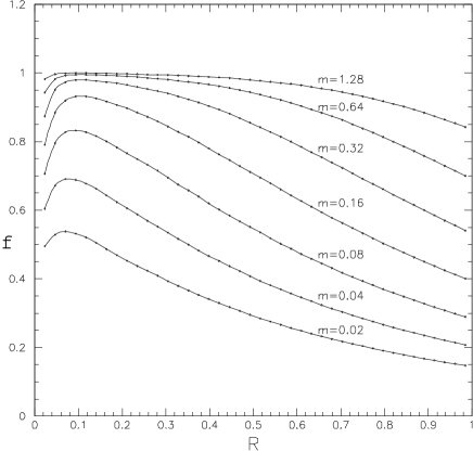
Figure 4: The relative contribution of the disk to the total radial force as a function of radius for the Newtonian-plus-dark-matter cases

In order to make a quantitative comparison between the growth rates of the unstable modes of the different mass models we scale the time step in the simulation in proportion to a natural dynamical time of the model. In Figure 5 are plotted, for each model, the ratio of the angular frequency of the $M=0.005$ mass model to to that of the specific model. As can be seen from the graph this ratio depends somewhat on R. We have chosen to scale the time step in proportion to the orbital time at $R=0.5$ (scaling the time step in proportion to orbital time at $R=0.25$ does not change the results qualitatively).

Figure 5: The ratio of the angular frequency of the $m=0.005$ mass model to the angular frequencies of all the mass models as a function of radius

The development of the instability is traced in the time dependence of the fraction of the disk’s mass in the m=2 Fourier component of the surface density. This turns out to have a period of exponential growth. We take the exponential growth rate as a measure of the instability’s strength. In Figure 6 we plot the growth rates as functions of mass for both the MOND and the Newtonian-plus-DM models. These are also given in Table 1 together with the Q value and the halo mass (for the Newtonian counterparts) of the different models. The growth rates are calculated using the scaled time units i.e. the real growth rate equals the growth rate that appears in the graph times $\Omega_{m}(R=0.5)/\Omega_{0.005}(R=0.5)$ as was described previously.

Figure 6: The growth rate, in units of the dynamical frequency, for the m=2 mode as a function of the total mass of the disk. $\Box$ MOND, $\triangle$ Newtonian + Halo.

4 Conclusions

From the results presented in Figure 3 we see that exponential disks having a given fraction of their kinetic energy in random motion, and a constant $Q$ profile are locally more stable in MOND than in Newtonian dynamics, as reflected in the fact that for the same value for $T/|W|$ the MOND disks have a higher $Q$ value. This is in agreement with the general result (Milgrom (1989)) regarding the local stability of disks in MOND. One can see that the change in the dynamics occurs when one crosses over from the Newtonian regime to the MOND regime i.e. when the acceleration in the disk become of the order of $a_{0}$. The added degree of stability is limited (the change in $Q$ saturates deep in the MOND regime). This stems from the fact that at both the Newtonian limit and the deep MOND limit the equations governing the evolution of the system obey simple (but different) scaling laws. The basic physical mechanism behind the added stability is the relatively weaker response in the potential to a given perturbation in the surface density when one is in the MOND regime. Roughly speaking in MOND $a^{2}\propto\rho$ and therefore $\delta a/a=\delta\rho/2\rho$, while in the Newtonian case $\delta a/a=\delta\rho/\rho$, and we see that approximately a factor of two is gained in stability.

From the results presented in Figure 6 and Table 1 we see that the global stability of the disk behaves in a way similar to the local stability. As one moves from the Newtonian regime to the MOND regime the growth rate of the $m=2$ mode (in dynamical-frequency units) decreases. At first (down to $M\sim 0.2$) the effect of MOND is similar to that of the added inertial halo. Below that the degree of stability continues to increase, but not as fast as that of the Newtonian disk-plus-halo; and it saturates in the deep MOND limit. In contrast, the Newtonian disk-in-halo becomes increasingly stable in the limit. The saturated global stability given the disk by MOND, is similar to that given a Newtonian disk by an inert halo with a mass that is 2-3 times the mass of the disk up to $R=5$ scale lengths. These results support the idea that pure MOND disks with high surface densities are less stable than those with a lower surface density both globally, and locally. This provides a possible explanation of the Freeman law as discussed in the introduction. It must, however, be appreciated that we cannot be sure that actual LSB galaxies are more stable than HSB ones because we do not know that they all have similar $T/W$ values, as used in our comparison.

Our aim in the paper has been to compare the stability properties in MOND of disks with different accelerations. In this, the Newtonian models have served as references so that the added MOND stability could be described in terms of an added inert halo. But, what is the significance of the comparison between the MOND and Newtonian disks as regards true galaxies? The disk-plus-inert-halo models we use are not what MOND predicts for a galaxy. If MOND is correct than in the low acceleration limit there should also appear to be much disk dark matter. In the present paper we have ignored the structure and motion in the z direction, perpendicular to the disk. A Newtonian model that will give the same 3-dimensional disk distribution function as a MOND pure disk, would have much disk dark matter that is not inert, but responds to disk perturbations. Put differently, MOND predicts that the dynamically determined surface density of LSB galaxies will be much higher than the observed surface density. When this surface density is used in calculating the Newtonian $Q$ value, as it should, a much lower $Q$ value will result in general (Milgrom (1989)). Inasmuch as we neglect the z-structure and take the disk as infinitely thin the exact value of the Newtonian surface density that gives the same potential field as MOND is $\Sigma_{N}=\Sigma/\mu^{+}$, where $\mu^{+}$ is the value of $\mu$ for the local acceleration just above the disk (because at every point on the disk, and at all times during its evolution, we have $\mu^{+}\partial_{n}\phi=2\pi G\Sigma$, while $2\pi G\Sigma_{N}=\partial_{n}\phi$). The net result is that even in the deep-MOND limit MOND disks are expected to be somewhat more stable than the Newtonian disks that have the same distribution function (and which thus have the same r- and z-structure) because of the $(1+L)^{1/2}$ factor. We do not include here simulations for such Newtonian models.

Appendix A Model construction

The problem of finding a distribution function (DF) $f(E,L_{z})$ can be made well posed for numerical solution by formulating it as a constrained optimization problem (see Binney and Tremaine (1987)). One wants a DF that satisfies the following physical requirements as constraints

$$f\geq 0,$$

$$\int fd{\bf v}=\Sigma(r),$$ (A1)

$$\int fv_{r}^{2}d{\bf v}/\int fd{\bf v}=\sigma_{vr}^{2}(r),$$

and, as an additional auxiliary constraint that will assure uniqueness, maximizes a certain functional of $f$ such as the Boltzmann entropy or some measure of smoothness. A very similar approach is to minimize a single functional of $f$ that is the sum of the errors in the surface density, the radial velocity dispersion, and the entropy, subject to the constrain that $f\geq 0$. We have used the latter approach. We take the disk to be a finite disk whose surface density vanishes for $r\geq 1$. The three input functions: the potential, the surface density, and the desired radial velocity dispersion, are represented by one dimensional arrays $\phi_{i}$, $\Sigma_{i}$, and $\sigma_{vr_{i}}$, respectively, at the equidistant grid point $r_{i}=i/N$ ($0\leq i\leq N$).

Using the variables

$$X=\frac{L_{z}^{2}}{2}-E+\phi(1),~{}~{}~{}Y=\frac{L_{z}^{2}}{2},$$ (A2)

and given a distribution function $f$, the surface density and radial velocity dispersion runs take the forms:

$$\Sigma^{\prime}(r) = \int\int f(X,Y)W(X,Y,r)dXdY,$$ (A3)

$$\sigma^{\prime\,2}_{vr}(r) = \Sigma^{\prime-1}(r)\int\int f(X,Y)W(X,Y,r)Z(X,Y,r)dXdY,$$ (A4)

$$W(X,Y,r) = Y^{-1/2}\{r^{2}[\phi(1)-\phi(r)-X]-(1-r^{2})Y\}^{-1/2}$$

$$Z(X,Y,r) = v^{2}_{r}(r)=2[Y(1-r^{-2})-X+\phi(1)-\phi(r)]$$

$$0\leq X \leq\phi(1)-\phi(r)$$

$$0\leq Y \leq\frac{r^{2}}{1-r^{2}}[\phi(1)-\phi(r)-X].$$

Note that we work here with the choice $R_{cut}=1$; more generally we would have to replace $L_{z}$ in the above expressions by $L_{z}/R_{cut}$.

Before discretizing the equations we make a change of variables from $X,Y$ to $r_{min},r_{max}$, which denote, respectively, the pericenter, and apocenter of an orbit with given energy and angular momentum. The transformation from $r_{min},r_{max}$ coordinates to the $X,Y$ coordinates can be obtained by solving the two equations:

$$Y = \frac{r_{min}^{2}}{1-r_{min}^{2}}[\phi(1)-\phi(r_{min})-X],$$ (A5)

$$Y = \frac{r_{max}^{2}}{1-r_{max}^{2}}[\phi(1)-\phi(r_{max})-X].$$ (A6)

From the expressions $X(r_{min},r_{max})$ and $Y(r_{min},r_{max})$ we calculate numerically the Jacobian $\frac{\partial(X,Y)}{\partial(r_{min},r_{max})}$ and rewrite the integrals (A3, A4) using the new coordinates where now the limits of integration are:

$$0 \leq r_{min}\leq r,$$ (A7)

$$r \leq r_{max}\leq 1.$$ (A8)

We also replace $\Sigma^{\prime}(r)$ in equation (A4) by the desired surface density, $\Sigma(r)$, since the two become identical when a solution is found. We discretize the DF on a Cartesian grid where

$$f_{jk}=f(r_{max_{j}},r_{min_{k}})$$ (A9)

$$r_{max_{j}}=(j-1)/N$$

$$r_{min_{k}}=(k-1)/N$$

and the value of f in between grid points is defined using bilinear interpolation. Since interpolation is linear in $f_{jk}$ and the integrals in eqs. (A3,A4), after the replacement of $\Sigma^{\prime}$, are also linear in $f_{jk}$, we can obtain expressions of the form:

$$\Sigma_{i}^{\prime} = \sum_{j,k}A_{ijk}\>f_{jk},$$ (A10)

$$\sigma_{vr_{i}}^{\prime\,2} = \sum_{j,k}B_{ijk}\>f_{jk}/\Sigma_{i},$$ (A11)

where $A_{ijk}$ and $B_{ijk}$ are calculated by numerically integrating
$\frac{\partial(X,Y)}{\partial(r_{min},r_{max})}W(X,Y,r)$ and $\frac{\partial(X,Y)}{\partial(r_{min},r_{max})}W(X,Y,r)Z(X,Y,r)$ respectively, over the relevant volume for each grid point. We are left with the discrete problem of minimizing the expression

$$a_{1}\sum_{i=1}^{N}\left(\Sigma_{i}-\Sigma_{i}^{\prime}\right)^{2}+a_{2}\sum_{i=1}^{N}\left(\sigma_{vr_{i}}^{2}-\sigma_{vr_{i}}^{\prime\,2}\right)^{2}+a_{3}S[f]$$ (A12)

with respect to the variables $f_{jk}$ given $\Sigma_{i}$ and $\sigma^{2}_{vr_{i}}.$ The functionals of $f$ that we have used are the Boltzmann entropy which is defined as $S=-\int f\log fd{\bf x}d{\bf v}$, or a measure of smoothness which we took as the $L^{2}$ norm of the gradient of f in the $r_{min}$, $r_{max}$ coordinates. After discretization we are left with an expression of the form

$$S=\sum_{j,k}C_{jk}\>f_{jk}\log(f_{jk})$$ (A13)

for the Boltzmann entropy, and an expression of the form

$$S=\sum_{j,k}D_{jk}[\left(f_{jk}-f_{j+1~{}k}\right)^{2}+\left(f_{jk}-f_{j~{}k+1}\right)^{2}]$$ (A14)

for the smoothness functional. We minimize (A12) using an iterative scheme where at each step we make a Gauss-Seidel relaxation sweep, we sweep over the grid, and at each grid point we set a new value for $f_{jk}$ in such a way that it will minimize eq. (A12) using a quadratic approximation obtained from the first and second derivatives of eq. (A12) with respect to $f_{jk}$. After each relaxation sweep we decrease the weight $a_{3}$ by multiplying it by a number smaller than one. In this way we let $a_{3}$ tend towards zero as the calculation progresses. In Figure 7 we plot as solid curves the input constraints of the surface density and the square of the radial velocity dispersion and as points the values calculated from a numerical solution found for the distribution function. The galaxy model is a smoothly truncated exponential disk having a total mass of 0.005, a constant $Q=2.55$, and obeys MOND. These models are described in section 3 As can be clearly seen from the graph the relaxation converges to an accurate solution.

Figure 7: The surface density and the square of the radial velocity dispersion for the $m=0.005$, $Q=2.55$, MOND, truncated exponential disk. The solid line represents the model and the dots are the numerical values calculated from the distribution function.

In Figure 8 we plot the distribution in phase space using $r_{min}-r_{max}$ coordinates of 500,000 particles according to a distribution function found for the model. In Figure 8 we plot the distribution in phase space using $r_{min}-r_{max}$ coordinates of 500,000 particles according to a distribution function found for the model.

Figure 8: The distribution of particles in phase space for a Q=2.55, MOND, truncated exponential disk model having a total of 500,000 particles.

Appendix B An N-body simulation and initial conditions

The nonlinearity of gravity in MOND prevents one from using most standard potential solvers, at least in a straightforward manner. Since we have written a multigrid potential solver it is a natural choice to use the particle-mesh algorithm, as described, e.g. in Hockney and Eastwood (1988), for N-body simulations. At each time step the density is interpolated from the particles to the grid; then we solve for the potential on the grid and interpolate the forces computed on the grid to the particle’s location in order to integrate its equations of motion. We use the cloud in a cell (CIC) charge assignment and multi-linear interpolation for the force calculation at the particle’s location; this algorithm is relatively fast. The same program can perform a simulation using MOND or Newtonian dynamics.

The potential solvers and the N-body code were extensively tested using Newtonian dynamics and MOND. Once the potential solver has been tested as described at the end of section 2 and found accurate there is no difference between Newtonian dynamics and MOND in the rest of the N-body code. The N-body code was tested by running stable King models, both Newtonian and MOND models, and observing the stationarity of the different quantities such as the size of the system, average velocities, total angular momentum, linear momentum, energy, etc. Kalnajs (1978) reported the eigenfrequencies of the dominant bisymmetric eigenmodes of the isochrone/$m_{k}$ models. Earn and Sellwod (1995) used Kalnajs’s distribution functions for the isochrone/12,9 models to compare the results they got from their expansion code to the analytic results of Kalnajs. We have run a simulation using our code, Newtonian dynamics, and their initial conditions. We then performed the same fit as they did for the pattern speeds and growth rates of the unstable modes. The fit between the numerical results and the analytical results were good (about 10-15% accuracy).

The importance of a careful initial setup for an equilibrium model is well documented (Sellwood (1983, 1987)). There are two separate aspects to this: suppression of particle noise and choosing coordinates from the desired distribution function. Initial positions picked randomly produce shot-noise density fluctuations on all scales. For initial, near-equilibrium models the initial behavior is dominated by the collective response to the artificial noise, and this can mask the dominant modes of the continuous system (Sellwood (1983)), in which we are interested. Such initial noise can be suppressed by arranging the particles regularly. This results in a discrete noise spectrum with large amplitudes at the wavelength of the particle spacing, which must be suppressed during the force determination. This would give a particle distribution that behaves as a smooth fluid. To this end, for our polar grid we place particles on rings spaced in radius according to the required surface density law. The number of particles on each ring must be related to the number of azimuthal Fourier harmonics $m_{max}$ that enters to the force. To prevent coupling of modes through aliases, $2(m_{max}+1)$ particles are needed on each ring. Quiet starts are also possible for warm stellar disks, but it is not practicable to suppress both radial and azimuthal density variations at the same time (Sellwood (1983); Sellwood and Athanassoula (1986)). Noise in the azimuthal forces must be suppressed since we are interested in non-axisymmetric instabilities. One then gives the particles on the ring identical velocity components so that the initial orbits remain congruent.

Choosing integrals of motion for each particle at random from the distribution function will result in statistical fluctuation about the intended function. These can be eliminated by choosing integrals for each particle in a deterministic manner such that their distribution is as close as possible to the required form. For example, one can use energy and angular momentum as the independent variables (Sellwood and Athanassoula (1986)); however, any other set of isolating integrals in which the distribution function can be expressed would work equally well.

Since we are interested in making a quantitative and systematic comparison between the stability of bare disks obeying MOND, and Newtonian disks with dark halos we want to minimize the statistical noise and employ a quiet start technique. As discussed above, one needs to use only a selected number of azimuthal Fourier components of $\Sigma$ in the force determination. In Newtonian dynamics this is justified for linear stability analysis since the Poisson equation and the linearized collisionless Boltzmann equation do not couple modes with different azimuthal frequencies. The MOND field equation can be linearized around the solution of the unperturbed axisymmetric disk (as discussed in Milgrom (1989)) and together with the linearized collisionless Boltzmann equation have the property that unstable modes with different azimuthal Fourier components are uncoupled. Instead of using the linearized MOND equation we use the full MOND equation, but leave only the desired Fourier components in the surface density that is assigned to the grid. In setting up the initial conditions we use the following procedure: We take the numerical solution obtained for the distribution function and interpolate it to a finer grid. We then calculate the number of particles that should reside in each cell given the total number of particles. This number is usually not an integer, we take the integer part and distribute the particles uniformly in the cell. The remaining fraction is interpreted as the probability for an additional particle to reside in this cell. We then draw cells at random according to their relative probabilities and place at most one additional particle in a cell. At the end of this stage we have a list of the $(r_{min},r_{max})$ coordinates of the particles. We now need to assign the phase-space coordinates for each particle i.e. $r,\theta,v_{r},v_{\theta}$. (Here we use a polar grid in the mid-plane as an auxiliary for computing the discretized density distribution that serves as input for the MOND field equation.) We draw randomly the radial position of the particle taking the probability density of finding the particle at radius $r$ as being proportional to $v_{r}^{-1}$. If we decide to use the Fourier filtering we draw at random the angle $\theta$ and place $2(m_{max}+1)$ particles at angular spacings of $\pi(m_{max}+1)^{-1}$ adding a small random angular shift to each particle to seed the unstable modes. If we do not use the Fourier filtering we place the particle at a random angle $\theta$ requiring that the surface density produced on the grid that is used by the potential solver will be as smooth as possible.

m Q time step Growth rate halo mass scaling MOND Newt+DM at R=1 0.005 2.55 1 0.01 2.5 0.84 0.4 0.02 2.4 0.7 0.43 0.04 2.25 0.58 0.46 0.09 0.18 0.08 2.0 0.48 0.51 0.36 0.23 0.16 1.79 0.39 0.62 0.53 0.28 0.32 1.62 0.3 0.8 0.8 0.31 0.64 1.53 0.22 0.94 0.94 0.31 1.28 1.5 0.16 1.0 0.97 0.27

Table 1: The growth rate, in units of dynamical frequency, for the $m=2$ mode, and model parameters for the different mass models.

References

- Bai and Brandt (1987) Bai, D. and Brandt, A. 1987, SIAM J. Sci. Stat. Comput., 8, No.2,