To appear in Physics Reports E-Print astro-ph/9811011
Origin and Propagation of Extremely High Energy Cosmic Rays
Pijushpani Bhattacharjee111e-mail:
pijush@iiap.ernet.in
Indian Institute of Astrophysics, Bangalore-560 034, India.
Günter Sigl222e-mail: sigl@humboldt.uchicago.edu
Astronomy & Astrophysics Center, Enrico Fermi Institute, University of Chicago,
5640 South Ellis Avenue, Chicago, IL 60637, USA
Cosmic ray particles with energies in excess of eV have been detected. The sources as well as the physical mechanism(s) responsible for endowing cosmic ray particles with such enormous energies are unknown. This report gives a review of the physics and astrophysics associated with the questions of origin and propagation of these Extremely High Energy (EHE) cosmic rays in the Universe. After a brief review of the observed cosmic rays in general and their possible sources and acceleration mechanisms, a detailed discussion is given of possible “top-down” (non-acceleration) scenarios of origin of EHE cosmic rays through decay of sufficiently massive particles originating from processes in the early Universe. The massive particles can come from collapse and/or annihilation of cosmic topological defects (such as monopoles, cosmic strings, etc.) associated with Grand Unified Theories or they could be some long-lived metastable supermassive relic particles that were created in the early Universe and are decaying in the current epoch. The highest energy end of the cosmic ray spectrum can thus be used as a probe of new fundamental physics beyond Standard Model. We discuss the role of existing and proposed cosmic ray, gamma-ray and neutrino experiments in this context. We also discuss how observations with next generation experiments of images and spectra of EHE cosmic ray sources can be used to obtain new information on Galactic and extragalactic magnetic fields and possibly their origin.
1 Introduction and Scope of This Review
The cosmic rays (CR) of Extremely High Energy (EHE) — those with energy [2, 3, 4, 7, 8, 9] — pose a serious challenge for conventional theories of origin of CR based on acceleration of charged particles in powerful astrophysical objects. The question of origin of these extremely high energy cosmic rays (EHECR)333We shall use the abbreviation EHE to specifically denote energies , while the abbreviation UHE for “Ultra-High Energy” will sometimes be used to denote 1 EeV, where 1 EeV = . Clearly UHE includes EHE but not vice versa. is, therefore, currently a subject of much intense debate and discussions; see Refs. [5, 6, 10], and Ref. [11] for a recent brief review.
The current theories of origin of EHECR can be broadly categorized into two distinct “scenarios”: the “bottom-up” acceleration scenario, and the “top-down” decay scenario, with various different models within each scenario. As the names suggest, the two scenarios are in a sense exact opposite of each other. In the bottom-up scenario, charged particles are accelerated from lower energies to the requisite high energies in certain special astrophysical environments. Examples are acceleration in shocks associated with supernova remnants, active galactic nuclei (AGNs), powerful radio galaxies, and so on, or acceleration in the strong electric fields generated by rotating neutron stars with high surface magnetic fields, for example. In the top-down scenario, on the other hand, the energetic particles arise simply from decay of certain sufficiently massive particles originating from physical processes in the early Universe, and no acceleration mechanism is needed.
The problems encountered in trying to explain the EHECR in terms of acceleration mechanisms have been well-documented in a number of studies; see, e.g., Refs. [12, 13, 14, 15]. Even if it is possible, in principle, to accelerate particles to EHECR energies of order 100 EeV in some astrophysical sources, it is generally extremely difficult in most cases to get the particles come out of the dense regions in and/or around the sources without losing much energy. Currently, the most favorable sources in this regard are perhaps a class of powerful radio galaxies (see, e.g., Refs. [16, 17, 18, 19, 20, 21] for recent reviews and references to literature), although the values of the relevant parameters required for acceleration to energies 100 EeV are somewhat on the side of extreme [14]. However, even if the requirements of energetics are met, the main problem with radio galaxies as sources of EHECR is that most of them seem to lie at large cosmological distances, 100 Mpc, from Earth. This is a major problem if EHECR particles are conventional particles such as nucleons or heavy nuclei. The reason is that nucleons above 70 EeV lose energy drastically during their propagation from the source to Earth due to Greisen-Zatsepin-Kuzmin (GZK) effect [22, 23], namely, photo-production of pions when the nucleons collide with photons of the cosmic microwave background (CMB), the mean-free path for which is few Mpc [24]. This process limits the possible distance of any source of EHE nucleons to 100 Mpc. If the particles were heavy nuclei, they would be photo-disintegrated [25, 26] in the CMB and infrared (IR) background within similar distances (see Sect. 4 for details). Thus, nucleons or heavy nuclei originating in distant radio galaxies are unlikely to survive with EHECR energies at Earth with any significant flux, even if they were accelerated to energies of order 100 EeV at source. In addition, since EHECR are hardly deflected by the intergalactic and/or Galactic magnetic fields, their arrival directions should point back to their sources in the sky (see Sect. 4 for details). Thus, EHECR offer us the unique opportunity of doing charged particle astronomy. Yet, for the observed EHECR events so far, no powerful sources along the arrival directions of individual events are found within about 100 Mpc [27, 13].444Very recently, it has been suggested by Boldt and Ghosh [28] that particles may be accelerated to energies near the event horizons of spinning supermassive black holes associated with presently inactive quasar remnants whose numbers within the local cosmological universe (i.e., within a GZK distance of order 50 Mpc) may be sufficient to explain the observed EHECR flux. This would solve the problem of absence of suitable currently active sources associated with EHECR. A detailed model incorporating this suggestion, however, remains to be worked out.
There are, of course, ways to avoid the distance restriction imposed by the GZK effect, provided the problem of energetics is somehow solved separately and provided one allows new physics beyond the Standard Model of particle physics; we shall discuss those suggestions later in this review.
In the top-down scenario, on the other hand, the problem of energetics is trivially solved from the beginning. Here, the EHECR particles owe their origin to decay of some supermassive “X” particles of mass , so that their decay products, envisaged as the EHECR particles, can have energies all the way up to . Thus, no acceleration mechanism is needed. The sources of the massive X particles could be topological defects such as cosmic strings or magnetic monopoles that could be produced in the early Universe during symmetry-breaking phase transitions envisaged in Grand Unified Theories (GUTs). In an inflationary early Universe, the relevant topological defects could be formed at a phase transition at the end of inflation. Alternatively, the X particles could be certain supermassive metastable relic particles of lifetime comparable to or larger than the age of the Universe, which could be produced in the early Universe through, for example, particle production processes associated with inflation. Absence of nearby powerful astrophysical objects such as AGNs or radio galaxies is not a problem in the top-down scenario because the X particles or their sources need not necessarily be associated with any specific active astrophysical objects. In certain models, the X particles themselves or their sources may be clustered in galactic halos, in which case the dominant contribution to the EHECR observed at Earth would come from the X particles clustered within our Galactic Halo, for which the GZK restriction on source distance would be of no concern.
In this report we review our current understanding of some of the major theoretical issues concerning the origin and propagation of EHECR with special emphasis on the top-down scenario of EHECR origin. The principal reason for focusing primarily on the top-down scenario is that there already exists a large number of excellent reviews which discuss the question of origin of ultra-high energy cosmic rays (UHECR) in general and of EHECR in particular within the general bottom-up acceleration scenario in details; see, e.g., Refs. [12, 29, 17, 18, 19, 20, 21]. However, for completeness, we shall briefly discuss the salient features of the standard acceleration mechanisms and the predicted maximum energy achievable for various proposed sources of UHECR.
We would like to emphasize here that this is primarily a theoretical review; we do not discuss the experimental issues (for the obvious reason of lack of expertise), although, again, for completeness, we shall mention the major experimental techniques and briefly review the experimental results concerning the EHECR. For an excellent historical account of the early experimental developments and the first claim of detection of an EHECR event, see Ref. [30]. For reviews on UHECR experiments in general and various kinds of experimental techniques used in detecting UHECR, see Refs. [31, 32, 33]. For a review of the current experimental situation concerning EHECR, see the recent review by Yoshida and Dai [34]. Overviews of the various currently operating, up-coming, as well as proposed future EHECR experiments can be found, e.g., in Refs. [6, 10].
By focusing primarily on the top-down scenario, we do not wish to give the wrong impression that the top-down scenario explains all aspects of EHECR. In fact, as we shall see below, essentially each of the specific top-down models that have been studied so far has its own peculiar set of problems. Indeed, the main problem of the top-down scenario in general is that it is highly model dependent and invariably involves as-yet untested physics beyond the Standard Model of particle physics. On the other hand, it is precisely because of this reason that the scenario is also attractive — it brings in ideas of new physics beyond the Standard Model of particle physics (such as Grand Unification) as well as ideas of early-Universe cosmology (such as topological defects and/or massive particle production in inflation) into the realms of EHECR where these ideas have the potential to be tested by future EHECR experiments.
The physics and astrophysics of UHECR are intimately linked with the emerging field of neutrino astronomy as well as with the already established field of ray astronomy which in turn are important subdisciplines of particle astrophysics (for a review see, e.g., Ref. [35]). Indeed, as we shall see, all scenarios of UHECR origin, including the top-down models, are severely constrained by neutrino and ray observations and limits. We shall also discuss how EHECR observations have the potential to yield important information on Galactic and extragalactic magnetic fields.
The plan of this review is summarized in the Table of Contents.
Unless otherwise stated or obvious from the context, we use natural units with throughout.
2 The Observed Cosmic Rays
In this section we give a brief overview of CR observations in general. Since this is a very rich topic with a tradition of almost 90 years, only the most important facts can be summarized. For more details the reader is referred to recent monographs on CR [36, 37] and to rapporteur papers presented at the biennial International Cosmic Ray Conference (ICRC) (see, e.g., Refs. [38, 39, 40]) for updates on the data situation. The relatively young field of ray astrophysics which has now become an important subfield of CR astrophysics, can only be skimmed even more superficially and for more information the reader is referred to the proceedings of the Compton ray symposia and the ICRC and to Refs. [41, 42, 43], for example. We will only mention those ray issues that are relevant for UHECR physics. Similarly, the emerging field of neutrino astrophysics [44] will be discussed only in the context of ultra-high energies for which a possible neutrino component and its potential detection will be discussed later in this review.
2.1 Detection Methods at Different Energies
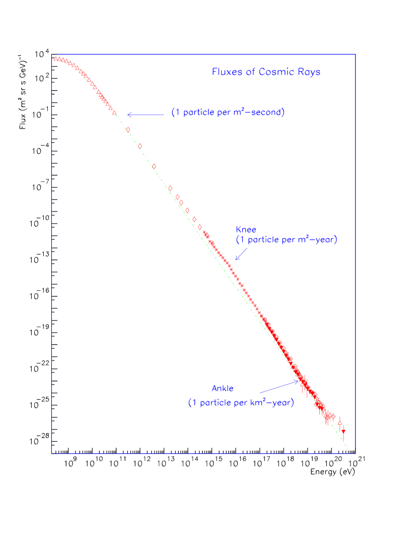
The CR primaries are shielded by the Earth’s atmosphere and near the ground reveal their existence only by indirect effects such as ionization. Indeed, it was the height dependence of this latter effect which lead to the discovery of CR by Hess in 1912. Direct observation of CR primaries is only possible from space by flying detectors with balloons or spacecraft. Naturally, such detectors are very limited in size and because the differential CR spectrum is a steeply falling function of energy, roughly in accord with a power-law with index up to an energy of eV (see Fig. 1), direct observations run out of statistics typically around a few TeV (eV) [45]. For the neutral component, i.e. rays, whose flux at a given energy is lower than the charged CR flux by several orders of magnitude, this statistical limit occurs at even lower energies, for example around GeV for the instruments on board the Compton Gamma Ray Observatory (CGRO) [46]. The space based detectors of charged CR traditionally use nuclear emulsion stacks such as in the JACEE experiment [47]; now-a-days, spectrometric techniques are also used which are advantageous for measuring the chemical composition. For rays, for example, the Energetic Gamma Ray Experiment Telescope (EGRET) on board the CGRO uses spark chambers combined with a NaI calorimeter.
Above roughly TeV, the showers of secondary particles created in the interactions of the primary CR with the atmosphere are extensive enough to be detectable from the ground. In the most traditional technique, charged hadronic particles, as well as electrons and muons in these Extensive Air Showers (EAS) are recorded on the ground [48] with standard instruments such as water Cherenkov detectors used in the old Volcano Ranch [2] and Haverah Park [4] experiments, and scintillation detectors which are used now-a-days. Currently operating ground arrays for UHECR EAS are the Yakutsk experiment in Russia [7] and the Akeno Giant Air Shower Array (AGASA) near Tokyo, Japan, which is the largest one, covering an area of roughly with about 100 detectors mutual separated by about km [9]. The Sydney University Giant Air Shower Recorder (SUGAR) [3] operated until 1979 and was the largest array in the Southern hemisphere. The ground array technique allows one to measure a lateral cross section of the shower profile. The energy of the shower-initiating primary particle is estimated by appropriately parametrizing it in terms a measurable parameter; traditionally this parameter is taken to be the particle density at 600 m from the shower core, which is found to be quite insensitive to the primary composition and the interaction model used to simulate air showers [49].
The detection of secondary photons from EAS represents a complementary technique. The experimentally most important light sources are the fluorescence of air nitrogen excited by the charged particles in the EAS and the Cherenkov radiation from the charged particles that travel faster than the speed of light in the atmosphere. The first source is practically isotropic whereas the second one produces light strongly concentrated on the surface of a cone around the propagation direction of the charged source. The fluorescence technique can be used equally well for both charged and neutral primaries and was first used by the Fly’s Eye detector [8] and will be part of several future projects on UHECR (see Sect. 2.6). The primary energy can be estimated from the total fluorescence yield. Information on the primary composition is contained in the column depth (measured in g) at which the shower reaches maximal particle density. The average of is related to the primary energy by
| (1) |
Here, is called the elongation rate and is a characteristic energy that depends on the primary composition. Therefore, if and are determined from the longitudinal shower profile measured by the fluorescence detector, then and thus the composition, can be extracted after determining the from the total fluorescence yield. Comparison of CR spectra measured with the ground array and the fluorescence technique indicate systematic errors in energy calibration that are generally smaller than 40%. For a more detailed discussion of experimental EAS analysis with the ground array and the fluorescence technique see, e.g., the recent review by Yoshida and Dai [34] and Refs. [31, 32, 33].
In contrast to the fluorescence light, for a given primary energy, the output in Cherenkov light is much larger for ray primaries than for charged CR primaries. In combination with the so called imaging technique — in which the Cherenkov light image of an electromagnetic cascade in the upper atmosphere (and thus also the primary arrival direction) is reconstructed [50] — the Cherenkov technique is one of the best tools available to discriminate rays from point sources against the strong background of charged CR. This technique is used, for example, by the High Energy Gamma Ray Astronomy (HEGRA) experiment (now 5 telescopes of 8.5 mirror area) [51] and by the 10 meter Whipple telescope [52] with threshold energies of GeV and GeV, respectively. In the Southern hemisphere, the Collaboration of Australia and Nippon (Japan) for a GAmma Ray Observatory in the Outback (CANGAROO) experiment [53] currently consists of two 7 meter imaging atmospheric Cherenkov telescopes at Woomera, Australia, with an energy threshold of 200 GeV.
Another new experiment which is at the completion stages of construction and testing is the Multi-Institution Los Alamos Gamma Ray Observatory (MILAGRO) [54] which is a water (rather than atmospheric)-Cherenkov detector that detects electrons, photons, hadrons and muons in EAS, has a 24-hour duty cycle, “all-sky” coverage, and good angular resolution ( at 10 TeV), and is sensitive to rays in the energy range from to . For rays, therefore, an as yet unexplored window between a few tens of GeV and GeV remains which may soon be closed by large-area atmospheric Cherenkov detectors [55]. For a detailed review of this field of very high energy ray astronomy see, e.g., Refs. [41, 42, 43].
Finally, muons of a few hundred GeV and above have penetration depths of the order of a kilometer even in rock and can thus be detected underground. The Monopole Astrophysics and Cosmic Ray Observatory (MACRO) experiment [56], for example, located in the Gran Sasso laboratory near Rome, Italy, has a rock overburden of about km, consists of tons of liquid scintillator and acts as a giant time-of-flight counter. Operated in coincidence with the Cherenkov telescope array EAS-TOP [57] located above it, it can for instance be used to study the primary CR composition around the “knee” region [58] (see Fig. 1). A similar combination is represented by the Antarctic Muon And Neutrino Detector Array (AMANDA) detector and the South Pole Air ShowEr array (SPASE) of scintillation detectors. AMANDA consists of strings of photomultiplier tubes of a few hundred meters in length deployed in the antarctic ice at depths of up to km, and reconstructs tracks of muons of energies in the TeV range [59].
2.2 The Measured Energy Spectrum
Fig. 1 shows a compilation of the CR all-particle spectrum over the whole range of energies observed through different experimental strategies as discussed in Sect. 2.1. The spectrum exhibits power law behavior over a wide range of energies, but comparison with a fit to a single power law (dashed line in Fig. 1) shows significant breaks at the “knee” at and, to a somewhat lesser extent, at the “ankle” at eV. The sharpness of the knee feature is a not yet resolved experimental issue, particularly because it occurs in the transition region between the energy range where direct measurements are available and the energy range where the data come from indirect detection by the ground array techniques whose energy resolution is typically 20% or worse [45]. For example, the EAS-TOP array observed a sharp spectral break at the knee within their experimental resolution [60], whereas the AGASA [61] and CASA-MIA [62] data support a softer transition.
Figs. 2–6 show the CR data above eV measured by different experiments. The ankle feature was first discussed in detail by the Fly’s Eye experiment [8]. The slope between the knee and up to eV is very close to 3.0 (Fig. 1); then it seems to steepen to about 3.2 up to the dip at eV, after which it flattens to about 2.7 above the dip. As will be discussed in Sect. 2.4, the Fly’s Eye also found evidence for a change in composition to a lighter component above the ankle, that is correlated with the change in spectral slope.
The situation at the high end of the CR spectrum is as yet inconclusive and represents the main subject of the recent strong increase of theoretical and experimental activities in UHECR physics which also motivated the present review. The present data (see Figs. 2–6) seem to reveal a steepening just below eV, but above that energy significantly more events have been seen than expected from an extrapolation of the GZK “cutoff” at eV. This is perhaps the most puzzling and hence interesting aspect of UHECR because a cutoff is expected at least for extragalactic nucleon primaries irrespective of the production mechanism (see Sect. 4.1). Even for conventional local sources, the maximal energy to which charged primaries can be accelerated is expected to be limited (see Sect. 5) and it is generally hard to achieve energies beyond the cutoff energy.
2.3 Events above eV
The first published event above eV was observed by the Volcano Ranch experiment [2]. The Haverah Park experiment reported 8 events around eV [4], and the Yakutsk array saw one event above this energy [7]. The SUGAR array in Australia reported 8 events above eV [3], the highest one at eV. The world record holder is still a eV event which was the only event above eV observed by the Fly’s Eye experiment [8], on 15 October 1991. Probably the second highest event at eV in the world data set was seen by the AGASA experiment [9] which meanwhile detected a total of 6 events above eV (see Fig. 2). The Fly’s Eye and the AGASA events have been documented in detail in the literature and it seems unlikely that their energy has been overestimated by more than 30%. For more detailed experimental information see, e.g., the review [34]. Theoretical and astrophysical implications of these events are a particular focus of the present review. For an overview of specific source searches for these events see Sect. 4.6.
2.4 Composition
We will discuss the question of composition here only for CR detected by ground based EAS detectors, i.e., for CR above TeV, only. Information on the chemical composition is mainly provided by the muon content in case of ground arrays and by the depth of shower maximum for optical observation of the EAS. Just to indicate the qualitative trend we mention that, for a given primary energy, a heavier nucleus produces EAS with a higher muon content and a shower maximum higher up in the atmosphere on average compared to those for a proton shower. The latter property can be understood by viewing a nucleus as a collection of independent nucleons whose interaction probabilities add, leading to a faster development of the shower on average. The higher muon content in a heavy nucleus shower is due to the fact that, because the shower develops relatively higher up in the atmosphere where the atmosphere is less dense, it is relatively easier for the charged pions in a heavy nucleus shower to decay to muons before interacting with the medium.
The spectral and compositional behavior around the knee at eV may play a crucial role in attempts to understand the origin and nature of CR in this energy range, as will be discussed in little more detail in Sect. 3. Indeed, there are indications that the chemical composition becomes heavier with increasing energies below the knee [45]. Around the knee the situation becomes less clear and most of the experimental results, such as from the SOUDAN-2 [63], the HEGRA [64], and the KArlsruhe Shower Core and Array DEtector (KASCADE) [65] experiments, seem to indicate a substantial proton component and no significant increase in primary mass. Recent results, for example, from the Dual Imaging Cherenkov Experiment (DICE) seem to indicate a lighter composition above the knee which may hint to a transition to a different component [66], but evidence for an inreasingly heavy composition above the knee has also been reported by the KASCADE collaboration [67] and by HEGRA [68].
Based on the analysis discussed above, Eq. (1), the Fly’s Eye collaboration reported a composition change from a heavy component below the ankle to a light component above, that is correlated with the spectral changes around the ankle [8]. However, this was not confirmed by the AGASA experiment [9, 34]. In addition, there have been suggestions that the observed energy dependence of could be caused by air shower physics rather than an actual composition change [69].
One signature of a heavy nucleus primary would be the almost simultaneous arrival of a pair of EASs at the Earth. Such pairs would be produced by photodisintegration of nuclei by solar photons and could be used to measure their mass, as was pointed out quite early on [70]. This effect has been reconsidered recently in light of existing and proposed UHECR detectors [71, 72].
At the highest energies, observed EAS seem to be consistent with nucleon primaries, but due to poor statistics and large fluctuations from shower to shower, the issue is not settled yet. Some scenarios of EHECR origin, such as the top-down scenario discussed in Sects. 6 and 7, predict the EHECR primaries to be dominated by photons and neutrinos rather than nucleons. Distinguishing between photon and nucleon induced showers is, however, extremely difficult at UHE and EHE regions — the standard muon-poorness criterion of photon induced showers relative to nucleon induced showers, applicable at lower ( – eV) energies, does not apply to the UHE region. It has been claimed that the highest energy Fly’s Eye event is inconsistent with a ray primary [73]. It should be noted, however, that at least for electromagnetic showers, EAS simulation at EHE is complicated by the Landau-Pomeranchuk-Migdal (LPM) effect and by the influence of the geomagnetic field [74]. Furthermore, in the simulations, EAS development depends to some extent on the hadronic interaction event generator which complicates data interpretation [75]. Definite conclusions on the composition of the EHECR, therefore, have to await data from next generation experiments. Together with certain characteristic features of the photon induced EHECR showers due to geomagnetic effects [74], the large event statistics expected from the next generation experiments will hopefully allow to distinguish between photon and nucleon EHECR primaries. In turn, accelerator data together with EAS data can be used to constrain, for example, the cross section of protons with air nuclei at center of mass energies of 30 TeV [76].
The hypothesis of neutrinos or new neutral particles as EHECR primaries will be discussed in Sect. 4.3.1 and 4.3.2, respectively.
2.5 Anisotropy
For a recent compilation and discussion of anisotropy measurements see Ref. [77]. Fig. 7 shows the summary figure from that reference. Implications of these anisotropy measurements will be discussed briefly in the next section where we discuss the origin of CR in general. For discussions of subtleties involved in the measurements and interpretation of anisotropy data, choice of coordinate systems used in presenting anisotropy results etc., see e.g., Ref. [31].
The anisotropy amplitude is defined as
| (2) |
where and are the minimum and maximum CR intensity as a function of arrival direction. Very recently, results have been presented on the anisotropy of the CR flux above eV from the Fly’s Eye [78] and the AGASA [79] experiments. Both experiments report a small but statistically significant anisotropy of the order of 4% in terms of Eq. (2) toward the Galactic plane at energies around eV. These analyses did not reveal a significant correlation with the Supergalactic Plane, whereas earlier work seemed to indicate some enhancement of the flux from this plane [80, 81, 82].
2.6 Next-generation Experiments on Ultrahigh Energy Cosmic Ray, Ray, and Neutrino Astrophysics
As an upscaled version of the old Fly’s Eye Cosmic Ray experiment, the High Resolution Fly’s Eye detector is currently under construction at Utah, USA [85]. Taking into account a duty cycle of about 10% (a fluorescence detector requires clear, moonless nights), the effective aperture of this instrument will be , about 10 times the AGASA aperture, with a threshold around eV. Another project utilizing the fluorescence technique is the Japanese Telescope Array [86] which is currently in the proposal stage. Its effective aperture will be about 15-20 times that of AGASA above eV, and it can also be used as a Cherenkov detector for TeV ray astrophysics. Probably the largest up-coming project is the international Pierre Auger Giant Array Observatories [87] which will be a combination of a ground array of about 1700 particle detectors mutually separated from each other by about 1.5 km and covering about , and one or more fluorescence Fly’s Eye type detectors. The ground array component will have a duty cycle of nearly 100%, leading to an effective aperture about 200 times as large as the AGASA array, and an event rate of 50–100 events per year above eV. About 10% of the events will be detected by both the ground array and the fluorescence component and can be used for cross calibration and detailed EAS studies. The energy threshold will be around eV. For maximal sky coverage it is furthermore planned to construct one site in each hemisphere. The southern site will be in Argentina, and the northern site probably in Utah, USA.
Recently NASA initiated a concept study for detecting EAS from space [88] by observing their fluorescence light from an Orbiting Wide-angle Light-collector (OWL). This would provide an increase by another factor in aperture compared to the Pierre Auger Project, corresponding to an event rate of up to a few thousand events per year above eV. Similar concepts such as the AIRWATCH [89] and Maximum-energy air-Shower Satellite (MASS) [90] missions are also being discussed. The energy threshold of such instruments would be between and eV. This technique would be especially suitable for detection of very small event rates such as those caused by UHE neutrinos which would produce horizontal air showers (see Sect. 7.4). For more details on these recent experimental considerations see Ref. [10].
New experiments are also planned in ray astrophysics. The Gamma ray Large Area Space Telescope (GLAST) [91] detector is planned by NASA as an advanced version of the EGRET experiment, with an about 100 fold increase in sensitivity at energies between 10 MeV and 200 GeV. For new ground based ray experiments we mention the Very Energetic Radiation Imaging Telescope Array System (VERITAS) project [93] which consists of eight 10 meter optical reflectors which will be about two orders of magnitude more sensitive between 50 GeV and 50 TeV than WHIPPLE. A similar next generation atmospheric imaging Cherenkov system with up to 16 planned telescopes is the High Energy Stereoscopic System (HESS) project [94]. Furthermore, the Mayor Atmospheric Gamma-ray Imaging Cherenkov Telescope (MAGIC) project [95] aims to build a very large atmospheric imaging Cherenkov telescope with mirror area for detection of rays between 10 GeV and 300 GeV, i.e. within the as yet unexplored window of ray astrophysics. The CANGAROO experiment in Australia plans to upgrade to four 10 meter telescopes and lower the threshold to 100 GeV. Finally, another strategy to explore this window utilizes existing solar heliostat arrays, and is represented by the Solar Tower Atmospheric Cherenkov Effect Experiment (STACEE) [96] in the USA, the ChErenkov Low Energy Sampling & Timing Experiment (CELESTE) in France [97], and the German-Spanish Gamma Ray Astrophysics at ALmeria (GRAAL) experiment [98].
High energy neutrino astronomy is aiming towards a kilometer scale neutrino observatory. The major technique is the optical detection of Cherenkov light emitted by muons created in charged current reactions of neutrinos with nucleons either in water or in ice. The largest pilot experiments representing these two detector media are the now defunct Deep Undersea Muon and Neutrino Detection (DUMAND) experiment [99] in the deep sea near Hawai and the AMANDA experiment [59] in the South Pole ice. Another water based experiment is situated at Lake Baikal [100]. Next generation deep sea projects include the French Astronomy with a Neutrino Telescope and Abyss environmental RESearch (ANTARES) [102] and the underwater Neutrino Experiment SouthwesT Of GReece (NESTOR) project in the Mediterranean [103], whereas ICECUBE [104] represents the planned kilometer scale version of the AMANDA detector. Also under consideration are neutrino detectors utilizing techniques to detect the radio pulse from the electromagnetic showers created by neutrino interactions in ice [105]. This technique could possibly be scaled up to an effective area of and a prototype is represented by the Radio Ice Cherenkov Experiment (RICE) experiment at the South Pole [106]. The radio technique might also have some sensitivity to the flavor of the primary neutrino [107]. Neutrinos can also initiate horizontal EAS which can be detected by giant ground arrays such as the Pierre Auger Project [108, 109]. Furthermore, as mentioned above, horizontal EAS could be detected from space by instruments such as the the proposed OWL detector [88]. Finally, the search for pulsed radio emission from cascades induced by neutrinos or cosmic rays above eV in the lunar regolith could also lead to interesting limits [110]. More details on neutrino astronomy detectors are contained in Refs. [111, 44, 112], and some recent overviews on neutrino astronomy can be found in Ref. [113, 114].
3 Origin of Bulk of the Cosmic Rays: General Considerations
The question of origin of cosmic rays continues to be regarded as an “unsolved problem” even after almost ninety years of research since the announcement of their discovery in 1912. Although the general aspects of the question of CR origin are regarded as fairly well-understood now, major gaps and uncertainties remain, the level of uncertainty being in general a function that increases with energy of the cosmic rays.
The total CR energy density measured above the atmosphere is dominated by particles with energies between about 1 and 10 GeV. At energies below GeV the intensities are temporally correlated with the solar activity which is a direct evidence for an origin at the Sun. At higher energies, however, the flux observed at Earth exhibits a temporal anticorrelation with solar activity and a screening whose efficiency increases with the strength of the solar wind, indicating an origin outside the solar system. Several arguments involving energetics, composition, and secondary ray production suggest that the bulk of the CR between 1 GeV and at least up to the knee region (see Fig. 1) is confined to the Galaxy and is probably produced in supernova remnants (SNRs). Between the knee and the ankle the situation becomes less clear, although the ankle is sometimes interpreted as a cross over from a Galactic to an extragalactic component. Finally, beyond EeV, CR are generally expected to have an extragalactic origin due to their apparent isotropy, but ways around this reasoning have also been suggested.
In the following, we give a somewhat more detailed account of these general considerations, separating the discussion into issues related to energetics, Galactic versus extragalactic origin, and acceleration mechanisms and the possible sources of CR. We reserve a more comprehensive discussion of the origin of UHECR above eV (which make only a small part of the total CR energy density, but are the main focus of this review) for Sects. 5 and 6.
3.1 Energetics
As mentioned above, the bulk of the CR observed at the Earth is of extrasolar origin. The average energy density of CR is thus expected to be uniform at least throughout most of the Galaxy. If CR are universal, their density should be constant throughout the whole Universe. As a curiosity we note in this context that the mean energy density of CR, , is comparable to the energy density of the CMB. It is not clear, however, what physical process could lead to such an “equilibration”, which is thus most likely just a coincidence. We will see in the following that indeed a universal origin of bulk of the CR is now-a-days not regarded as a likely possibility.
If the CR accelerators are Galactic, they must replenish for the escape of CR from the Galaxy in order to sustain the observed Galactic CR differential intensity . Their total luminosity in CR must therefore satisfy , where is the mean residence time of CR with energy in the Galaxy and is the volume. can be estimated from the mean column density, , of gas in the interstellar medium that Galactic CR with energy have traversed. Interaction of the primary CR particles with the gas in the interstellar medium leads to production of various secondary species. From the secondary to primary abundance ratios of Galactic CR it was infered that [115]
| (3) |
where is the mean density of interstellar gas and is the mean charge number of the CR particles. The mean energy density of CR and the total mass of gas in the Milky Way that have been inferred from the diffuse Galactic ray, X-ray and radio emissions are and , respectively. Hence, simple integration yields
| (4) |
This is about 10% of the estimated total power output in the form of kinetic energy of the ejected material in Galactic supernovae which, from the energetics point of view, could therefore account for most of the CR. We note that the energy release from other Galactic sources, e.g. ordinary stars [36] or isolated neutron stars [116] is expected to be too small, even for UHECR555This conclusion may, however, change somewhat with the recent detection of certain soft-gamma repeaters [117] which seem to indicate the existence of a subclass of pulsars with dipole magnetic fields as large as a few times G. This may increase the available magnetic energy budget from pulsars by two to three orders of magnitude.. Together with other considerations (see Sect. 3.2) this leads to the widely held notion that CR at least up to the knee predominantly originate from first-order Fermi acceleration (see below) in SNRs.
Another interesting observation is that the energy density in the form of CR is comparable both to the energy density in the Galactic magnetic field (G) as well as that in the turbulent motion of the gas,
| (5) |
where and are the density and turbulent velocity of the gas, respectively. This can be expected from a pressure equilibrium between the (relativistic) CR, the magnetic field, and the gas flow. If Eq. (5) roughly holds not only in the Galaxy but also throughout extragalactic space, then we would expect the extragalactic CR energy density to be considerably smaller than the Galactic one which is another argument in favor of a mostly Galactic origin of the CR observed near Earth (see Sect.3.2). We note, however, that, in order for Eq. (5) to hold, typical CR diffusion time-scale over the size of the system under consideration must be smaller than its age. This is not the case, for example, in clusters of galaxies if the bulk of CR are produced in the member galaxies or in cluster accretion shocks [118].
3.2 Galactic versus Extragalactic Origin of the Bulk of the CR
The energetical considerations mentioned above already provide some arguments in favor of a Galactic origin of the bulk of the CR. Another argument involves the production of secondary rays from the decays of neutral pions produced in interactions of CR with the baryonic gas throughout the Universe: For given densities of the CR and the gas, the resulting ray flux can be calculated quite reliably [119] and the predictions can be compared with observations. This has been done, for example, for the Small Magellanic Cloud (SMC). The observed upper limits [120] turn out to be a factor of a few below the predictions assuming a universal CR density. The CR density at the SMC should, therefore, be at least a factor of a few smaller than the local Galactic density.
As a second test we mention the search for a CR gradient (e.g., [121, 122, 123]: For a Galactic CR origin one expects a decrease of CR intensity with increasing distances from the Galactic center which should be encoded in the secondary ray emission that can be measured by space based instruments such as EGRET. The observational situation is, however, not completely settled yet [124]. Whereas the spatial variation of the ray flux fits rather well, the observed spectrum appears to be too flat compared to the one expected from the average CR spectrum. Since the average CR spectrum throughout the Galaxy is generally steepened (compared to the spectrum at the source) by diffusion in Galactic magnetic fields, the observed relatively flat secondary ray spectrum may be interpreted as if the secondary rays are produced by CR interactions mainly at the (Galactic) sources rather than in the interstellar medium. This interpretation, however, requires that the escape time of CR from their sources be energy-independent.
Some information on CR origin is in principle also contained in the distribution of their arrival directions which has been discussed in Sect. 2.5 (see Fig. 7). Below eV, the amplitude of the observed anisotropy, , is statistically significant and roughly energy independent. Above eV, observed anisotropy amplitudes are generally statistically insignificant with possible exceptions between eV and eV [77] and again close to eV, the latter correlated with the Galactic plane [78, 79]. A possible clustering towards the Supergalactic Plane for energies above a few tens of EeV was claimed [80, 81, 82], but has not been confirmed by more recent studies [78, 79]. Since charged CR at these energies are hardly deflected by the Galactic magnetic field, the apparent lack of any significant anisotropy associated with the Galactic plane implies that the high energy end of the CR spectrum is most likely to have an extragalactic origin (see Sect. 4.6).
For Galactic sources, detailed models of CR diffusion and ray production in the Galaxy have been developed (see, e.g., Ref. [126]). These models are generally based on the energy loss - diffusion equation that will be discussed below in the context of UHECR propagation [see Eq. (36)], with the diffusion constant generalized to a diffusion tensor. This tensor and other parameters in these models can be obtained from fits to the observed abundances of nuclear isotopes. It is often sufficient to consider a simplified model, the so called “leaky box” model (see Refs. [36, 37] for detailed discussions) in which the diffusion term is approximated by a loss term involving a CR containment time . Fits to the data lead to yr below eV with only a weak energy dependence. This is in turn consistent with observed anisotropies which, below eV, can be interpreted by the Compton-Getting effect [127] which describes the effect of the motion of the observer relative to an isotropic distribution of CR. In this case the relative motion is a combination of the motion of the solar system within the Galaxy and the drift motion of the charged CR diffusing and/or convecting in the interstellar medium. The magnitude and the weak energy dependence of the anisotropy in this energy range can be interpreted as arising out of diffusion of CR predominantly along the tangled incoherent component of the Galactic magnetic field. In summary, CR composition and anisotropy data provide further evidence for a Galactic origin for energies at least up to the knee region of the spectrum.
In this context, the knee itself is often interpreted as a magnetic deconfinement effect such that CR above the knee leave the Galaxy relatively faster, leading to steepening of the spectrum above the knee. In addition, the maximum energy achieved in shock acceleration is proportional to the primary charge and could also lead to a spectral steepening (see Sect. 3.3). Alternatively, the knee has also been interpreted as being caused by the flux contribution from a strong single source [128].
Finally, since the range of electrons above eV becomes smaller than due to synchrotron and inverse Compton losses, the electronic CR component at such energies, which is about 1% of the hadronic flux, is undoubtedly of Galactic origin. This can also be explained by acceleration in SNRs.
3.3 Acceleration Mechanisms and Possible Sources
There are basically two kinds of acceleration mechanisms considered in connection with CR acceleration: (1) direct acceleration of charged particles by an electric field, and (2) statistical acceleration (Fermi acceleration) in a magnetized plasma.
In the direct acceleration mechanism, the electric field in question can be due, for example, to a rotating magnetic neutron star (pulsar) or, a (rotating) accretion disk threaded by magnetic fields, etc. The details of the actual acceleration process and the maximum energy to which a particle can be accelerated depend on the particular physical situation under consideration. For a variety of reasons, the direct acceleration mechanisms are, however, not widely favored these days as the CR acceleration mechanism. Apart from disagreements among authors about the crucial details of the various models, a major disadvantage of the mechanism in general is that it is difficult to obtain the characteristic power-law spectrum of the observed CR in any natural way. However, as pointed out by Colgate [129], a power law spectrum does not necessarily point to Fermi acceleration, but results whenever a fractional gain in energy of a few particles is accompanied by a significantly larger fractional loss in the number of remaining particles. We will not discuss the direct acceleration mechanism in any more details, and refer the reader to reviews, e.g., in Ref. [36, 12, 16, 129].
The basic idea of the statistical acceleration mechanism originates from a paper by Fermi [130] in 1949: Even though the average electric field may vanish, there can still be a net transfer of macroscopic kinetic energy of moving magnetized plasma to individual charged particles (“test particles”) in the medium due to repeated collisionless scatterings (“encounters”) of the particles either with randomly moving inhomogeneities of the turbulent magnetic field or with shocks in the medium. Fermi’s original paper [130] considered the former case, i.e., scattering with randomly moving magnetized “clouds” in the interstellar medium. In this case, although in each individual encounter the particle may either gain or lose energy, there is on average a net gain of energy after many encounters. The original Fermi mechanism is now-a-days called “second-order” Fermi mechanism, because the average fractional energy gain in this case is proportional to , where is the relative velocity of the cloud with respect to the frame in which the CR ensemble is isotropic, and is the velocity of light. Because of the dependence on the square of the cloud velocity (), the second-order Fermi mechanism is not a very efficient acceleration process. Indeed, for typical interstellar clouds in the Galaxy, the acceleration time scale turns out to be much larger than the typical escape time ( years) of CR in the Galaxy deduced from observed isotopic ratios of CR. In addition, although the resulting spectrum of particles happens to be a power-law in energy, the power-law index depends on the cloud velocity, and so the superposed spectrum due to many different sources with widely different cloud velocities would not in general have a power-law form.
A more efficient version of Fermi mechanism is realized when one considers encounters of particles with plane shock fronts. In this case, the average fractional energy gain of a particle per encounter (defined as a cycle of one crossing and then a re-crossing of the shock after the particle is turned back by the magnetic field) is of first order in the relative velocity between the shock front and the isotropic-CR frame. Currently, the “standard” theory of CR acceleration — the so-called “Diffusive Shock Acceleration Mechanism” (DSAM) is, therefore, based on this first-order Fermi acceleration mechanism at shocks. For reviews and references to original literature on DSAM, see, e.g., Refs. [131, 132, 133, 16, 20, 21]. An important feature of DSAM is that particles emerge out of the acceleration site with a characteristic power-law spectrum with a power-law index that depends only on the shock compression ratio, and not on the shock velocity. Shocks are ubiquitous in astrophysical situations: in the interplanetary space, in supernovae in interstellar medium, and even in cosmological situations as in radio-galaxies. The basic ideas of the DSAM have received impressive confirmation from in-situ observations in the solar system, in particular, from observations of high energy particles accelerated at the Earth’s bow shock generated by collision of the solar wind with the Earth’s magnetosphere; see, again the reviews in Refs. [131, 132, 133, 16] for references. We will discuss the DSAM again in connection with UHECR in Sect. 5. Here we only note that for a given acceleration site, there is a maximum energy achievable, , which is limited either by the size of the shock (which has to be larger than the gyroradius of the particles being accelerated) or by the time scale of acceleration up to this energy (which has to be smaller than the lifetime of the shock and also smaller than the shortest time-scale of energy losses).
From a theoretical point of view, SNRs are not only attractive (and maybe the only serious) candidate of Galactic CR origin in terms of power (see Sect. 3.1) but also in terms of the maximum achievable CR energy, which is estimated to lie somewhere between eV and eV. In addition, the observed constant beryllium-to-iron abundance ratio in the atmospheres of stars of different metallicity is another indicator that at least the carbon, nitrogen and oxygen CR, that produce beryllium by spallation with interstellar hydrogen and helium (this being the main production channel for beryllium), have to be accelerated in SNRs [134]. For recent discussions of the relevance of composition for the origin of Galactic CR, see Refs. [135] for lithium, beryllium, and boron in particular, and Refs. [136] in general.
The DSAM theory of CR acceleration in SNRs has been worked out in considerable details; see, e.g., Refs. [131, 132, 137, 138]. Support to the shock-acceleration scenario for hadronic CR is given by experimental indications that while the composition below the knee region becomes heavier with energy (see Sect. 2.4), the composition is relatively less dependent on rigidity (, where is the momentum and is the charge, and is the speed of light). This is expected for shock acceleration for which the maximum rigidity should be equal for all nuclei. Furthermore, the observed X-ray emission from SNRs seems to be caused by synchrotron radiation of electrons with energies up to TeV. Assuming that nuclei are accelerated as well, this implies fluxes consistent with Galactic CR acceleration in SNR shocks [139].
As another effect, the interactions with the surrounding matter of protons accelerated in SNRs produce neutral pions, and the resulting flux of secondary rays from SNRs has been predicted as well; see, e.g., Ref [140, 141, 142, 143, 144, 145]. Nowadays, given the existence of space and ground based ray detecting systems (see Sect. 2.1), the SNR acceleration paradigm for Galactic CR origin can also be tested by searching for these secondary rays. As of now, the situation is still somewhat inconclusive since no firm detection of such rays has been reported (see, e.g., Ref. [146, 147]). Furthermore, the SNR scenario almost certainly does not explain UHECR which consequently would constitute a separate component. Pulsars and neutron stars in close binary systems have also been discussed as alternative Galactic CR sources for which the maximum energy in principle may even reach the UHECR energy range. However, an origin of the bulk of the cosmic rays in X-ray binary systems is contradicted by the complete absence of detectable TeV radiation from Cygnus X-3 and Hercules X-1, as reported by the Chicago Air Shower Array-MIchigan Anti (CASA-MIA) experiment [148].
A comprehensive scenario for the origin of CR based exclusively on first-order Fermi acceleration has been proposed by Biermann [17]. In this scenario, the sources are (a) supernovae exploding into the interstellar medium, for energies up to eV, (b) supernovae exploding into a predecessor stellar wind, for energies up to eV, and (c) the hot spots of powerful radio-galaxies for the highest energies. It is claimed that this scenario meets every observational test to date.
A criticism of shock acceleration as the origin of CR has been given by Colgate [129]. Instead, acceleration in the electric fields produced by reconnection of twisted magnetic fields has been suggested as a mechanism that could operate in a much larger fraction in space than shock acceleration and up to the highest observed CR energies. This is due to the wide-spread presence of helical magnetic fields carrying excess angular momentum from mass condensations in the Universe. Apart from proposed laboratory experiments [129], it is, however, presently not clear how to observationally discriminate this scenario of CR origin from the shock acceleration scenario. Also, the power law index of the predicted spectra does not fall out of this scenario naturally and may strongly depend on the specific environment.
Plaga [149] has presented a scenario where all extrasolar hadronic CR are extragalactic in origin and accumulate in the Galaxy due to “magnetic flux trapping”. It was claimed that the ray flux levels from the Magellanic clouds is not a suitable test of this scenario and that the ankle in the energy spectrum appears as a natural consequence of this scenario.
The opposite possibility that all CR nuclei above a few GeV and up to the highest energies observed, and all electrons and rays above a few MeV are of Galactic origin has also been put forward by Dar and collaborators [150]. In this scenario the acceleration sources have been suggested to be the hot spots in the highly relativistic jets from merger and accretion induced collapse of compact stellar objects, the so called microblazars, within our own Galaxy and its halo. The same objects in external galaxies could also give rise to cosmological ray bursts.
Finally, to close this short summary with a very speculative possibility of CR origin, we note that it is known that charged and/or polarizable particles interacting with the electromagnetic zero-point fluctuations are accelerated stochastically [151, 152]. The discussion of this effect goes back to Einstein and Hopf [153] who investigated classical atoms interacting with classical thermal radiation. The acceleration rate for a proton is given by [151]
| (6) |
where is the radiation damping constant, the nucleon mass, and is a frequency that is smaller than the Compton frequencies of the quarks. In an energy range where energy losses are negligible, the resulting acceleration spectrum must have the form due to the Lorentz invariance of the spectrum of the vacuum fluctuations. The latter is also the reason that a net acceleration results because it implies the absence of a drag force. The spectrum typically cuts off exponentially at energies where the acceleration time becomes larger than the proton attenuation time at that same energy due to loss processes. It seems, however, unlikely that this acceleration process plays a significant role in CR production because, for given typical baryon densities, the predicted hard spectrum tends to overproduce CR fluxes at high energies.
4 Propagation and Interactions of Ultra-High Energy Radiation
Since implications and predictions of the spectrum of UHECR depend on their composition which is uncertain, we will in this chapter review the propagation of all types of particles that could play the role of UHECR. We start with the hadronic component, continue with discussion on electromagnetic cascades initiated by UHE photons in extragalactic space, and then comment on more exotic options such as UHE neutrinos and new neutral particles predicted in certain supersymmetric models of particle physics. We then discuss how propagation can be influenced by cosmic magnetic fields and what constraints on the location of UHECR sources are implied. The role played by these constraints in the search for sources of EHECR beyond eV is discussed. Finally, the formal description of CR propagation by transport equations is briefly reviewed, with an account of the literature on analytical and numerical approaches to their solution.
Before proceeding, we set up some general notation. The interaction length of a CR of energy and mass propagating through a background of particles of mass is given by
| (7) |
where is the number density of the background particles per unit energy at energy , and are the velocities of the background particle and the CR, respectively, is the cosine of the angle between the incoming momenta, and is the total cross section of the relevant process for the squared center of mass (CM) energy
| (8) |
The most important background particles turn out to be photons with energies in the infrared and optical (IR/O) range or below, so that we will usually have , . A review of the universal photon background has been given in Ref. [154].
It proves convenient to also introduce an energy attenuation length that is obtained from Eq. (7) by multiplying the integrand with the inelasticity, i.e. the fraction of the energy transferred from the incoming CR to the recoiling final state particle of interest. The inelasticity is given by
| (9) |
where is the energy of the recoiling particle considered in units of the incoming CR energy . Here by recoiling particle we usually mean the “leading” particle, i.e. the one which carries most of the energy.
If one is mostly interested in this leading particle, the detailed transport equations (see Sect. 4.7) for the local density of particles per unit energy, , are often approximated by the simple “diffusion equation”
| (10) |
in terms of the energy loss rate and the local injection spectrum . Eq. (10) applies to a particle which loses energy at a rate , and is often referred to as the continuous energy loss (CEL) approximation. The CEL approximation is in general good if the non-leading particle is of a different nature than the leading particle, and if the inelasticity is small, . For an isotropic source distribution in the matter-dominated regime for a flat Universe (), Eq. (10) yields a differential flux today at energy , , as
| (11) |
where is the age of the Universe, is the energy at injection redshift in the CEL approximation, i.e. the solution of (with including loss due to redshifting), with . The maximum redshift corresponds either to an absolute cutoff of the source spectrum at or to the earliest epoch when the source became active, whichever is smaller. For a homogeneous production spectrum , this simplifies to
| (12) |
if is much smaller than the horizon size such that redshift and evolution effects can be ignored. Eqs. (11) and (12) are often used in the literature for approximate flux calculations.
4.1 Nucleons, Nuclei, and the Greisen-Zatsepin-Kuzmin Cutoff
Shortly after its discovery, it was pointed out by Greisen [22] and by Zatsepin & Kuzmin [23] that the cosmic microwave background (CMB) radiation field has profound consequences for UHECR: With respect to the rest frame of a nucleon that has a sufficiently high energy in the cosmic rest frame (CRF, defined as the frame in which the CMB is isotropic), a substantial fraction of the CMB photons will appear as rays above the threshold energy for photo-pion production, MeV. The total cross section for this process as a function of the ray energy in the nucleon rest frame, , is shown in Fig. 8. Near the threshold the cross section exhibits a pronounced resonance associated with single pion production, whereas in the limit of high energies it increases logarithmically with [155]. The long tail beyond the first resonance is essentially dominated by multiple pion production, , ( stands for the background photon). For a background photon of energy in the CRF, the threshold energy translates into a corresponding threshold for the nucleon energy,
| (13) |
Typical CMB photon energies are eV, leading to the so called Greisen-Zatsepin-Kuzmin (GZK) “cutoff” at a few tens of EeV where the nucleon interaction length drops to about Mpc as can be seen in Fig. 9. Detailed investigations of differential cross sections, extending into the multiple pion production regime, have been performed in the literature, mainly for the purpose of calculating secondary ray and neutrino production; for recent discussions and references to earlier literature see, e.g., Refs. [156, 157, 158].
Below this energy range, the dominant loss mechanism for protons is production of electron-positron pairs on the CMB, , down to the corresponding threshold
| (14) |
Therefore, pair production by protons (PPP) in the CMB ensues at a proton energy eV. The first detailed discussion of PPP in astrophysics was given by Blumenthal [159]. PPP is very similar to triplet pair production by electrons, (see Sect. 4.2.), where “electron”, , means either an electron or a positron in the following. Away from the threshold the total cross section for a nucleus of charge is well approximated by the one for triplet pair production, multiplied by . Parametric fits to the total cross section and the inelasticity for PPP over the whole energy range were given in Ref. [160]. The resulting proton attenuation length is shown in Fig. 9. The next important loss mechanism which starts to dominate near and below the PPP threshold is redshifting due to the cosmic expansion. Indeed, all other loss processes are negligible, except possibly in very dense central regions of galaxies: The interaction length due to hadronic processes which have total cross sections of the order of 0.1 barn in the energy range of interest, for example, is Mpc, where [161], with the average cosmic baryon density in units of the critical density, and the Hubble constant in units of .
For neutrons, decay () is the dominant loss process for eV. The neutron decay rate , with sec the laboratory lifetime, implies a neutron range of propagation
| (15) |
The dominant loss process for nuclei of energy eV is photodisintegration [25, 26, 162, 163] in the CMB and the IR background (IRB) due to the giant dipole resonance. Early calculations [26] suggested a loss length of a few Mpc. Recent observations of multi-TeV rays from the BL Lac objects Mrk 421 and Mrk 501 suggest [164, 165], however, an IRB roughly a factor 10 lower than previously assumed, which is also consistent with recent independent calculation [166] of the intensity and spectral energy distribution of the IRB based on empirical data primarily from IRAS galaxies. This tends to increase the loss length for nuclei [167]. Recent detailed Monte Carlo simulations [168, 169, 170] indicate that, with the reduced IR background, the CMB becomes the dominant photon background responsible for photodisintegration and, for example, leads to a loss length of Mpc at eV. This loss length plays an important role for scenarios in which the highest energy events observed are heavy nuclei that have been accelerated to UHE (see, e.g., Ref. [27]): The accelerators can not be much further away than a few tens of Mpc. Specific flux calculations for the source NGC 253 have been performed in Ref. [171]. Apart from photodisintegration, nuclei are subject to the same loss processes as nucleons, where the respective thresholds are given by substituting by the mass of the nucleus in Eqs. (13) and (14).
4.2 UHE Photons and Electromagnetic Cascades
As in the case of UHE nucleons and nuclei, the propagation of UHE photons (and electrons/positrons) is also governed by their interaction with the cosmic photon background. The dominant interaction processes are the attenuation (absorption) of UHE photons due to pair-production (PP) on the background photons : [172], and inverse Compton scattering (ICS) of the electrons (positrons) on the background photons. Early studies of the effect of PP attenuation on the cosmological UHE -ray flux can be found, e.g., in Refs. [173].
The ray threshold energy for PP on a background photon of energy is
| (16) |
whereas ICS has no threshold. In the high energy limit, the total cross sections for PP and ICS are
| (17) |
For , approaches the Thomson cross section ( is the fine structure constant), whereas peaks near the threshold Eq. (16). Therefore, the most efficient targets for electrons and rays of energy are background photons of energy . For UHE this corresponds to MHz. Thus, radio background photons play an important role in UHE -ray propagation through extragalactic space.
Unfortunately, the universal radio background (URB) is not very well known mostly because it is difficult to disentangle the Galactic and extragalactic components. Observational estimates have been given in Ref. [174], and an early theoretical estimate was given in Ref. [175]. Recently, an attempt has been made to calculate the contribution to the URB from radio-galaxies and AGNs [176], and also from clusters of galaxies [177] which tends to give higher estimates. The issue does not seem to be settled, however. At frequencies somewhere below MHz the URB is expected to cut off exponentially due to free-free absorption. The exact location of the cut-off depends on the abundance and clustering of electrons in the intergalactic medium and/or the radio source and is uncertain between about MHz. Fig. 10 compares results from Ref. [176] with Ref. [175] and the observational estimate from Ref. [174].
In the extreme Klein-Nishina limit, , either the electron or the positron produced in the process carries most of the energy of the initial UHE photon. This leading electron can then undergo ICS whose inelasticity (relative to the electron) is close to 1 in the Klein-Nishina limit. As a consequence, the upscattered photon which is now the leading particle after this two-step cycle still carries most of the energy of the original ray, and can initiate a fresh cycle of PP and ICS interactions. This leads to the development of an electromagnetic (EM) cascade which plays an important role in the resulting observable ray spectra. An important consequence of the EM cascade development is that the effective penetration depth of the EM cascade, which can be characterized by the energy attenuation length of the leading particle (photon or electron/positron), is considerably greater than just the interaction lengths [178]; see Figs. 11 and 12). As a result, the predicted flux of UHE photons can be considerably larger than that calculated by considering only the absorption of UHE photons due to PP.
EM cascades play an important role particularly in some exotic models of UHECR origin such as collapse or annihilation of topological defects (see Sect. 6) in which the EHECR injection spectrum is predicted to be dominated by -rays [179]. Even if only UHE nucleons and nuclei are produced in the first place, for example, via conventional shock acceleration (see Sect. 5), EM cascades can be produced by the secondaries coming from the decay of pions which are created in interactions of UHE nucleons with the low energy photon background.
The EM cascading process and the resulting diffuse -ray fluxes in the conventional acceleration scenarios of UHECR origin were calculated in the ’70s; see, e.g., Refs. [180, 181, 182]. The EM cascades initiated by “primary” -rays and their effects on the diffuse UHE -ray flux in the topological defect scenario of UHECR were first considered in Ref. [179]. All these calculations were performed within the CEL approximation which, as described above, deals with only the leading particle. However, the contribution of non-leading particles to the flux can be substantial for cascades that are not fully developed. A reliable calculation of the flux at energies much smaller than the maximal injection energy should therefore go beyond the CEL approximation, i.e., one should solve the relevant Boltzmann equations for propagation; this is discussed in Sect. 4.7.
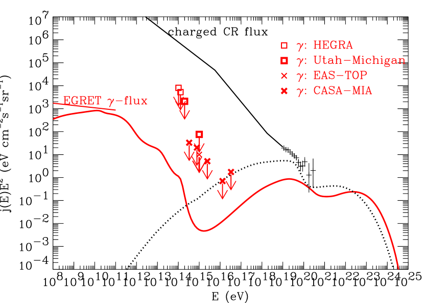
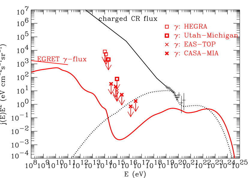
Cascade development accelerates at lower energies due to the decreasing interaction lengths (see Figs. 11 and 12) until most of the rays fall below the PP threshold on the low energy photon background at which point they pile up with a characteristic spectrum below this threshold [36, 183, 184, 185]. The source of these rays are predominantly the ICS photons of average energy arising from interactions of electrons of energy with the background at average squared CM energy in the Thomson regime. The relevant background for cosmological propagation is constituted by the universal IR/O background, corresponding to eV in Eq. (16), or eV. Therefore, most of the energy of fully developed EM cascades ends up below GeV where it is constrained by measurements of the diffuse ray flux by EGRET on board the CGRO [186] and other effects (see Sect. 7). Flux predictions involving EM cascades are therefore an important source of constraints of UHE energy injection on cosmological scales. This is further discussed in Sects. 6 and 7.
It should be mentioned here that the development of EM cascades depends sensitively on the strength of the extragalactic magnetic fields (EGMFs) which is rather uncertain. The EGMF typically inhibits cascade development because of the synchrotron cooling of the pairs produced in the PP process. For a sufficiently strong EGMF the synchrotron cooling time scale of the leading electron (positron) may be small compared to the time scale of ICS interaction, in which case, the electron (positron) synchrotron cools before it can undergo ICS, and thus cascade development stops. In this case, the UHE -ray flux is determined mainly by the “direct” -rays, i.e., the ones that originate at distances less than the absorption length due to PP process. The energy lost through synchrotron cooling does not, however, disappear; rather, it reappears at lower energies and can even initiate fresh EM cascades there depending on the remaining path length and the strength of the relevant background photons. Thus, the overall effect of a relatively strong EGMF is to deplete the UHE -ray flux above some energy and increase the flux below a corresponding energy in the “low” (typically few tens to hundreds of GeV) energy region. These issues are further discussed in Sect. 4.4.1.
The lowest order cross sections, Eq. (17), fall off as for . Therefore, at EHE, higher order processes with more than two final state particles start to become important because the mass scales of these particles can enter into the corresponding cross section which typically is asymptotically constant or proportional to powers of .
Double pair production (DPP), , is a higher order QED process that affects UHE photons. The DPP total cross section is a sharply rising function of near the threshold that is given by Eq. (16) with , and quickly approaches its asymptotic value [187]
| (18) |
DPP begins to dominate over PP above eV, where the higher values apply for stronger URB (see Fig. 11).
For electrons, the relevant higher order process is triplet pair production (TPP), . This process has been discussed in some detail in Refs. [188] and its asymptotic high energy cross section is
| (19) |
with an inelasticity of
| (20) |
Thus, although the total cross section for TPP on CMB photons becomes comparable to the ICS cross section already around eV, the energy attenuation is not important up to eV because (see Fig. 12). The main effect of TPP between these energies is to create a considerable number of electrons and channel them to energies below the UHE range. However, TPP is dominated over by synchrotron cooling (see Sect. 4.4), and therefore negligible, if the electrons propagate in a magnetic field of r.m.s. strength G, as can be seen from Fig. 12.
Various possible processes other than those discussed above — e.g., those involving the production of one or more muon, tau, or pion pairs, double Compton scattering (), scattering (), Bethe-Heitler pair production (, where stands for an atom, an ion, or a free electron), the process , and photon interactions with magnetic fields such as pair production () — are in general negligible in EM cascade development. The total cross section for the production of a single muon pair (), for example, is smaller than that for electron pair production by about a factor 10. Energy loss rate contributions for TPP involving pairs of heavier particles of mass are suppressed by a factor for . Similarly, DPP involving heavier pairs is also negligible [187]. The cross section for double Compton scattering is of order and must be treated together with the radiative corrections to ordinary Compton scattering of the same order. Corrections to the lowest order ICS cross section from processes involving additional photons in the final state, , , turn out to be smaller than 10% in the UHE range [189]. A similar remark applies to corrections to the lowest order PP cross section from the processes , . Photonphoton scattering can only play a role at redshifts beyond and at energies below the redshift-dependent pair production threshold given by Eq. (16) [190, 191, 192]. A similar remark applies to Bethe-Heitler pair production [191]. Photon interactions with magnetic fields of typical galactic strength, G, are only relevant for eV [193]. For extragalactic magnetic fields (EGMFs) the critical energy for such interactions is even higher.
4.3 Propagation and Interactions of Neutrinos and “Exotic” Particles
4.3.1 Neutrinos
Neutrino propagation
The propagation of UHE neutrinos is governed mainly by their interaction with the relic neutrino background (RNB). The average squared CM energy for interaction of an UHE neutrino of energy with a relic neutrino of energy is given by
| (21) |
If the relic neutrino is relativistic, then in Eq. (21), where eV is the temperature at redshift and is the dimensionless chemical potential of relativistic relic neutrinos. For nonrelativistic relic neutrinos of mass eV, . Note that Eq. (21) implies interaction energies that are typically smaller than electroweak energies even for UHE neutrinos, except for energies near the Grand Unification scale, GeV, or if eV. In this energy range, the cross sections are given by the Standard Model of electroweak interactions which are well confirmed experimentally. Physics beyond the Standard Model is, therefore, not expected to play a significant role in UHE neutrino interactions with the low energy relic backgrounds.
The dominant interaction mode of UHE neutrinos with the RNB is the exchange of a boson in the t-channel (), or of a boson in either the s-channel () or the t-channel () [194, 195, 196, 197]. Here, stands for either the electron, muon, or tau flavor, where for the first reaction, denotes a charged lepton, and any charged fermion. If the latter is a quark, it will, of course, subsequently fragment into hadrons. As an example, the differential cross section for s-channel production of is given by
| (22) |
where is the Fermi constant, and are mass and lifetime of the , and are the usual dimensionless left- and right-handed coupling constants for , and is the cosine of the scattering angle in the CM system.
The t-channel processes have cross sections that rise linearly with up to , with the mass, above which they are roughly constant with a value . Using Eq. (21) this yields the rough estimate
In contrast, within the Standard Model the neutrino-nucleon cross section roughly behaves as
| (24) |
for eV (see discussion below at end of Sect. 4.3.1). Interactions of UHE neutrinos with nucleons are, however, still negligible compared to interactions with the RNB because the RNB particle density is about ten orders of magnitude larger than the baryon density. The only exception could occur near Grand Unification scale energies and at high redshifts and/or if contributions to the neutrino-nucleon cross section from physics beyond the Standard Model dominate at these energies (see below at end of Sect. 4.3.1).
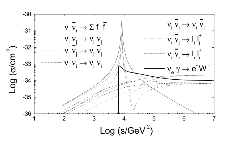
It has recently been pointed out [198] that above the threshold for production the process becomes comparable to the processes discussed above. Fig. 13 compares the cross sections relevant for neutrino propagation at CM energies around the electroweak scale. Again, for UHE neutrino interactions with the RNB the relevant CM energies can only be reached if (a) the UHE neutrino energy is close to the Grand Unification scale, or (b) the RNB neutrinos have masses in the eV regime, or (c) at redshifts . Even then the process never dominates over the process.
At lower energies there is an additional interaction that was recently discussed as potentially important besides the processes: Using an effective Lagrangian derived from the Standard Model, Ref. [199] obtained the result , supposed to be valid at least up to . Above the electron pair production threshold the cross section has not been calculated because of its complexity but is likely to level off and eventually decrease. Nevertheless, if the behavior holds up to a few hundred MeV2, comparison with Eq. (4.3.1) shows that the process would start to dominate and influence neutrino propagation around eV, as was pointed out in Ref. [200].
For a given source distribution, the contribution of the “direct” neutrinos to the flux can be computed by integrating Eq. (11) up to the interaction redshift , i.e. the average redshift from which a neutrino of present day energy could have propagated without interacting. This approximation neglects the secondary neutrinos and the decay products of the leptons created in the neutral current and charged current reactions of UHE neutrinos with the RNB discussed above. Similarly to the EM case, these secondary particles can lead to neutrino cascades developing over cosmological redshifts [196].
Approximate expressions for the interaction redshift for the processes discussed above have been given in Refs. [36, 201] for CM energies below the electroweak scale, assuming relativistic, nondegenerate relic neutrinos, , and . Approaching the electroweak scale, a resonance occurs in the interaction cross section for s-channel exchange at the mass, , see Eq. (22). The absorption redshift for the corresponding neutrino energy, drops to a few (or less for a degenerate, relativistic RNB) and asymptotically approaches constant values of a few tens at higher energies.
An interesting situation arises if the RNB consists of massive neutrinos with eV: Such neutrinos would constitute hot dark matter which is expected to cluster [202], for example, in galaxy clusters. This would potentially increase the interaction probability for any neutrino of energy within the width of the resonance at eV. Recently it has been suggested that the stable end products of the “Z-bursts” that would thus be induced at close-by distances () from Earth may explain the highest energy cosmic rays [203, 204] and may also provide indirect evidence for neutrino hot dark matter. These end products would be mostly nucleons and rays with average energies a factor of and lower, respectively, than the original UHE neutrino. As a consequence, if the UHE neutrino was produced as a secondary of an accelerated proton, the energy of the latter would have to be at least a few eV [203], making Z-bursts above GZK energies more likely to play a role in the context of non-acceleration scenarios (see Sects. 6,7). Moreover, it has subsequently been pointed out [205] that Z production is dominated by annihilation on the non-clustered massive RNB compared to annihilation with neutrinos clustering in the Galactic halo or in nearby galaxy clusters. As a consequence, for a significant contribution of neutrino annihilation to the observed EHECR flux, a new class of neutrino sources, unrelated to UHECR sources, seems necessary. This has been confirmed by more detailed numerical simulations [206] where it has, however, also been demonstrated that the most significant contribution could come from annihilation on neutrino dark matter clustering in the Local Supercluster by amounts consistent with expectations. In the absence of any assumptions on the neutrino sources, the minimal constraint comes from the unavoidable production of secondary rays contributing to the diffuse flux around 10 GeV measured by EGRET: If the Z-burst decay products are to explain EHECR, the massive neutrino overdensity over a length scale has to satisfy , provided that only neutrinos leave the source, a situation that may arise in top-down models if the X particles decay exclusively into neutrinos (see Ref. [207] for a model involving topological defects and Ref. [208] for a scenario involving decaying superheavy relic particles). If, instead, the total photon source luminosity is comparable to the total neutrino luminosity, as in most models, the EGRET constraint translates into the more stringent requirement . This bound can only be relaxed if most of the EM energy is radiated in the TeV range where the Universe is more transparent [206]. Furthermore, the Z-burst scenario requires sources that are optically thick for accelerated protons with respect to photo-pion production because otherwise the observable proton flux below the GZK cutoff would be comparable to the neutrino flux [205]. A systematic parameter study of the required overdensity, based on analytical flux estimates, has been performed in Ref. [209]. Recently it has been noted that a degenerate relic neutrino background would increase the interaction probability and thereby make the Z-burst scenario more promising [210]. A neutrino asymmetry of order unity is not excluded phenomenologically [211] and can be created in the early Universe, for example, through the Affleck-Dine baryogenesis mechanism [212] or due to neutrino oscillations. The authors of Ref. [210] pointed out that for a neutrino mass eV, a value suggested by the Super-Kamiokande experiment [213], and for sources at redshifts of a few, the flux of secondary Z-decay products is maximal for a RNB density parameter . Such neutrino masses, however, require the sources to produce neutrinos at least up to eV.
UHE neutrinos from the decay of pions, that are produced by interactions of accelerated protons in astrophysical sources, must have originated within redshifts of a few. Moreover, in most conventional models their flux is expected to fall off rapidly above eV. Examples are production in active galactic nuclei within hadronic models [214, 215, 216, 217, 218, 219], and “cosmogenic” neutrinos from interactions of UHECR nucleons (near or above the GZK cutoff) with the CMB (see, e.g.,Refs. [220, 221]). The latter source is the only one that is guaranteed to exist due to existence of UHECR near the GZK cutoff, but the fluxes are generally quite small. Therefore, interaction of these UHE neutrinos with the RNB, that could reveal the latter’s existence, can, if at all, be important only if the relic neutrinos have a mass eV [194]. Due to the continuous release of UHE neutrinos up to much higher redshifts, most top-down scenarios would imply substantially higher fluxes that also extend to much higher energies [201]. Certain features in the UHE neutrino spectrum predicted within such top-down scenarios, such as a change of slope for massless neutrinos [196] or a dip structure for relic neutrino masses of order eV [197, 204], have therefore been proposed as possibly the only way to detect the RNB. However, some of the scenarios at the high end of neutrino flux predictions have recently been ruled out based on constraints on the accompanying energy release into the EM channel (see Sect. 7).
Since in virtually all models UHE neutrinos are created as secondaries from pion decay, i.e. as electron or muon neutrinos, neutrinos can only be produced by a flavor changing t-channel interaction with the RNB. The flux of UHE neutrinos is therefore usually expected to be substantially smaller than the one of electron and muon neutrinos, if no neutrino oscillations take place at these energies. However, the recent evidence from the Superkamiokande experiment for nearly maximal mixing between muon and neutrinos with [213] would imply an oscillation length of pc and, therefore, a rough equilibration between muon and neutrino fluxes from any source at a distance larger than [222]. Turning this around, one sees that a source at distance emitting neutrinos of energy is sensitive to neutrino mixing with [223, 224]. Under certain circumstances, resonant conversion in the potential provided by the RNB clustering in galactic halos may also influence the flavor composition of UHE neutrinos from extraterrestrial sources [225]. In addition, such huge cosmological baselines can be sensitive probes of neutrino decay [226].
Neutrino detection
We now turn to a discussion of UHE neutrino interactions with matter relevant for neutrino detection. UHE neutrinos can be detected by detecting the muons produced in ordinary matter via charged-current reactions with nucleons; see, e.g., Refs. [227, 228, 231] for recent discussions. Corresponding cross sections are calculated by folding the fundamental standard model quark-neutrino cross section with the distribution function of the partons in the nucleon. These cross sections are most sensitive to the abundance of partons of fractional momentum , where is the neutrino energy. For the relevant squared momentum transfer, , these parton distribution functions have been measured down to [229]. (It has been suggested that observation of the atmospheric neutrino flux with future neutrino telescopes may probe parton distribution functions at much smaller currently inaccessible to colliders [230]). Currently, therefore, neutrino-nucleon cross sections for eV can be obtained only by extrapolating the parton distribution functions to lower . Above eV, the resulting uncertainty has been estimated to be a factor 2 [228], whereas within the dynamical radiative parton model it has been claimed to be at most 20 % [231]. An intermediate estimate using the CTEQ4-DIS distributions can roughly be parameterized by [228]
| (25) |
Improved calculations including non-leading logarithmic contributions in have recently been performed in Ref. [232]. The results for the neutrino-nucleon cross section differ by less than a factor 1.5 with Refs. [228, 231] even at eV. Neutral-current neutrino-nucleon cross sections are expected to be a factor 2-3 smaller than charged-current cross sections at UHE and interactions with electrons only play a role at the Glashow resonance, , at eV. Furthermore, cross sections of neutrinos and anti-neutrinos are basically identical at UHE. Radiative corrections influence the total cross section negligibly compared to the parton distribution uncertainties, but may lead to an increase of the average inelasticity in the outgoing lepton from to at eV [233], although this would probably hardly influence the shower character.
Neutrinos propagating through the Earth start to be attenuated above TeV due to the increasing Standard Model cross section as indicated by Eq. (25). Detailed integrations of the relevant transport equations for muon neutrinos above a TeV have been presented in Ref. [232], and, for a general cold medium, in Ref. [234]. In contrast, neutrinos with energy up to PeV can penetrate the Earth due to their regeneration from decays [224]. As a result, a primary UHE neutrino beam propagating through the Earth would cascade down below TeV and in a neutrino telescope could give rise to a higher total rate of upgoing events as compared to downgoing events for the same beam arriving from above the horizon. As mentioned above, a primary neutrino beam could arise even in scenarios based on pion decay, if mixing occurs with the parameters suggested by the Super-Kamiokande results [222]. In the PeV range, neutrinos can produce characteristec ”double-bang” events where the first bang would be due to the charged-current production by the neutrino of a whose decay at a typical distance 100 m would produce the second bang [223]. These effects have also been suggested as an independent astrophysical test of the neutrino oscillation hypothesis. In addition, isotropic neutrino fluxes in the energy range between 10 TeV and 10 PeV have been suggested as probes of the Earth’s density profile, whereby neutrino telescopes could be used for neutrino absorption tomography [235].
New Interactions
It has been suggested that the neutrino-nucleon cross section could be enhanced by new physics beyond the electroweak scale in the CM, or above about a PeV in the nucleon rest frame; see Eq. (21). For the lowest partial wave contribution to the cross section of a point-like particle this would violate unitarity [236]. However, two major possibilities have been discussed in the literature for which unitarity bounds seem not to be violated. In the first, a broken SU(3) gauge symmetry dual to the unbroken SU(3) color gauge group of strong interaction is introduced as the “generation symmetry” such that the three generations of leptons and quarks represent the quantum numbers of this generation symmetry. In this scheme, neutrinos can have effectively strong interaction with quarks and, in addition, neutrinos can interact coherently with all partons in the nucleon, resulting in an effective cross section comparable to the geometrical nucleon cross section [237]. However, the massive neutral gauge bosons of the broken generation symmetry would also mediate flavor changing neutral current (FCNC) processes, and experimental bounds on these processes indicate that the scale of any such new interaction must be above TeV. The second possibility is that there may be a large increase in the number of degrees of freedom above the electroweak scale [238]. A specific implementation of this idea is given in theories with additional large compact dimensions and a quantum gravity scale TeV that has recently received much attention in the literature [239] because it provides an alternative solution (i.e., without supersymmetry) to the hierarchy problem in Grand Unifications of gauge interactions. In such scenarios, the exchange of bulk gravitons (Kaluza-Klein modes) leads to an extra contribution to any two-particle cross section given by [240]
| (26) |
where the last expression applies to a neutrino of energy hitting a nucleon at rest. Note that a neutrino would typically start to interact in the atmosphere for , i.e. for eV, assuming TeV. The neutrino therefore becomes a primary candidate for the observed EHECR events. A specific signature of this scenario in neutrino telescopes based on ice or water as detector medium would be the absence of events above the energy where grows beyond . The corresponding signature in atmospheric detectors such as the Pierre Auger detectors would be a hardening of the spectrum above the energy .
There are, however, astrophysical constraints on which result from limiting the emission of bulk gravitons into the extra dimensions. The strongest constraints in this regard come from nucleon-nucleon bremsstrahlung in type II supernovae [241]. These contraints read TeV, TeV, and TeV, for , respectively, and, therefore, is required if neutrino primaries are to serve as a primary candidate for the EHECR events observed above eV. This assumes that all extra dimensions have the same size given by
| (27) |
where denotes the Planck mass. The above lower bounds on thus translate into the corresponding upper bounds mm, mm, and mm, respectively. The neutrino primary hypothesis of EHECR together with other astrophysical and cosmological constraints thus provides an interesting testing ground for theories involving large compact extra dimensions representing one possible kind of physics beyond the Standard Model. In this context, we mention that in theories with large compact extra dimensions mentioned above, Newton’s law of gravity is expected to be modified at distances smaller than the length scale given by Eq. (27). Indeed, there are laboratory experiments measuring gravitational interaction at small distances (for a recent review of such experiments see Ref. [242]), which also probe these theories. Thus, future EHECR experiments and gravitational experiments in the laboratory together have the potential of providing rather strong tests of these theories. These tests would be complementary to constraints from collider experiments [243].
In the context of conventional astrophysical sources, the relevant UHE neutrino primaries could, of course, only be produced as secondaries in interactions of accelerated protons of energies at least eV with matter or with low energy photons. This implies strong requirements on the possible sources (see Sect. 5).
4.3.2 Supersymmetric Particles
Certain supersymmetric particles have been suggested as candidates for the EHECR events. For example, if the gluino is light and has a lifetime long compared to the strong interaction time scale, because it carries color charge, it will bind with quarks, anti-quarks and/or gluons to form color-singlet hadrons, so-called R-hadrons. This can occur in supersymmetric theories involving gauge-mediated supersymmetry (SUSY) breaking [244] where the resulting gluino mass arises dominantly from radiative corrections and can vary between GeV and GeV. In these scenarios, the gluino can be the lightest supersymmetric particle (LSP). There are also arguments against a light quasi-stable gluino [245], mainly based on constraints on the abundance of anomalous heavy isotopes of hydrogen and oxygen which could be formed as bound states of these nuclei and the gluino. However, the case of a light quasi-stable gluino does not seem to be settled.
In the context of such scenarios a specific case has been suggested in which the gluino mass lies between 0.1 and GeV [246]. The lightest gluino-containing baryon, , denoted , could then be long-lived or stable, and the kinematical threshold for – “GZK” interaction would be higher than for nucleons, at an energy given by substituting the mass for the nucleon mass in Eq. (13) [247]. Furthermore, the cross section for – interaction peaks at an energy higher by a facor where the ratio of the mass splittings between the primary and the lowest lying resonance of the (of mass ) and the nucleon satisfies . As a result of this and a somewhat smaller interaction cross section of with photons, the effective GZK threshold is higher by factors of a few and sources of events above eV could be 15-30 times further away than for the case of nucleons. The existence of such events was, therefore, proposed as a signal of supersymmetry [247]. In fact, Farrar and Biermann reported a possible correlation between the arrival direction of the five highest energy CR events and compact radio quasars at redshifts between 0.3 and 2.2 [248], as might be expected if these quasars were sources of massive neutral particles. Undoubtedly, with the present amount of data the interpretation of such evidence for a correlation remains somewhat subjective, as is demonstrated by the criticism of the statistical analysis in Ref. [248] by Hoffman [249] and the reply by Farrar and Biermann [250]). Still, it can be expected that only a few more events could confirm or rule out the quasar hypothesis.
Meanwhile, however, accelerator constraints have become more stringent [251, 252] and seem to be inconsistent with the scenario from Ref. [246]. However, the scenario with a “tunable” gluino mass [244] still seems possible and suggests either the gluino–gluon bound state , called glueballino , or the isotriplet , called , as the lightest quasi-stable R-hadron. For a summary of scenarios with light gluinos consistent with accelerator constraints see Ref. [253].
Similar to the neutrino primary hypothesis in the context of acceleration sources (see Sect. 4.3.1), a specific difficulty of this scenario is the fact that, of course, the neutral R-hadron can not be accelerated, but rather has to be produced as a secondary of an accelerated proton interacting with the ambient matter. As a consequence, protons must be accelerated to at least eV at the source in order for the secondary particles to explain the EHECR events. Furthermore, secondary production would also include neutrinos and especially rays, leading to fluxes from powerful discrete acceleration sources that may be detectable in the GeV range by space-borne ray instruments such as EGRET and GLAST, and in the TeV range by ground based ray detectors such as HEGRA and WHIPPLE and the planned VERITAS, HESS, and MAGIC projects. At least the latter three ground based instruments should have energy thresholds low enough to detect rays from the postulated sources at redshift . Such observations in turn imply constraints on the required branching ratio of proton interactions into the R-hadron which, very roughly, should be larger than . These constraints, however, will have to be investigated in more detail for specific sources. It was also suggested to search for heavy neutral baryons in the data from Cherenkov instruments in the TeV range in this context [254].
A further constraint on new, massive strongly interacting particles in general comes from the character of the air showers created by them: The observed EHECR air showers are consistent with nucleon primaries and limits the possible primary rest mass to less than GeV [255]. With the statistics expected from upcoming experiments such as the Pierre Auger Project, this upper limit is likely to be lowered down to GeV.
It is interesting to note in this context that in case of a confirmation of the existence of new neutral particles in UHECR, a combination of accelerator, air shower, and astrophysics data would be highly restrictive in terms of the underlying physics: In the above scenario, for example, the gluino would have to be in a narrow mass range, 1–10 GeV, and the newest accelerator constraints on the Higgs mass, GeV, would require the presence of a D term of an anomalous gauge symmetry, in addition to a gauge-mediated contribution to SUSY breaking at the messenger scale [244].
Finally, SUSY could also play a role in top-down scenarios where it would modify the spectra of particles resulting from the decay of the X particles (see Sect. 6.2.1).
4.3.3 Other Particles
Recently it was suggested that QCD instanton induced interactions between quarks can lead to a stable, strong bound state of two particles, a so called H-dibaryon state with a mass MeV [256]. This particle would have properties similar to the sypersymmetric particle discussed in the previous section, i.e. it is neutral and its spin is zero. Its effective GZK cutoff would, therefore, also be considerably higher than for nucleons, at approximately eV, according to Ref. [256]. It would thus also be a primary candidate for the observed EHECR events that could be produced at high redshift sources.
4.4 Signatures of Galactic and Extragalactic Magnetic Fields in UHECR Spectra and Images
Cosmic magnetic fields can have several implications for UHECR propagation that may leave signatures in the observable spectra which could in turn be used to constrain or even measure the magnetic fields in the halo of our Galaxy and/or the extragalactic magnetic field (EGMF).
4.4.1 Synchrotron Radiation and Electromagnetic Cascades
As already mentioned in Sect. 4.2, the development of EM cascades strongly depends on presence and strength of magnetic fields via the synchrotron loss of its electronic component: For a particle of mass and charge ( is the electron charge) the energy loss rate in a field of squared r.m.s. strength is
| (28) |
For UHE protons this is negligible, whereas for UHE electrons the synchrotron losses eventually dominate over their attenuation (due to interaction with the background photons) above some critical energy eV that depends somewhat on the URB (see Fig. 12). Cascade development above that energy is essentially blocked because the electrons lose their energy through synchrotron radiation almost instantaneously once they are produced. In this energy range, ray propagation is therefore governed basically by absorption due to PP or DPP, and the observable flux is dominated by the “direct” or “first generation” rays, and their flux can be calculated by integrating Eq. (11) up to the absorption length (or redshift). Since this length is much smaller than the Hubble radius, for a homogeneous source distribution this reduces to Eq. (12), with replaced by the interaction length .
Thus, for a given injection spectrum of rays and electrons for a source beyond a few Mpc, the observable cascade spectrum depends on the EGMF. As mentioned in Sect. 4.2, the hadronic part of UHECR is a continuous source of secondary photons whose spectrum may therefore contain information on the large scale magnetic fields [257]. This spectrum should be measurable down to eV if rays can be discriminated from nucleons at the level. In more speculative models of UHECR origin such as the topological defect scenario that predict domination of rays above eV, EGMFs can have even more direct consequences for UHECR fluxes and constraints on such scenarios (see Sect. 7.1).
The photons coming from the synchrotron radiation of electrons of energy have a typical energy given by
| (29) |
which is valid in the classical limit, . Constraints can arise when this energy falls in a range where there exist measurements of the diffuse ray flux, such as from EGRET around GeV [186], or upper limits on it, such as at TeV from HEGRA [258], and between eV and eV from CASA-MIA [259]. For example, certain strong discrete sources of UHE rays such as massive topological defects with an almost monoenergetic injection spectrum in a G EGMF would predict ray fluxes that are larger than the charged cosmic ray flux for some energies above eV and can therefore be ruled out [260].
4.4.2 Deflection and Delay of Charged Hadrons
Whereas for electrons synchrotron loss is more important than deflection in the EGMF, for charged hadrons the opposite is the case. A relativistic particle of charge and energy has a gyroradius where is the field component perpendicular to the particle momentum. If this field is constant over a distance , this leads to a deflection angle
| (30) |
Magnetic fields beyond the Galactic disk are poorly known and include a possible extended field in the halo of our Galaxy and a large scale EGMF. In both cases, the magnetic field is often characterized by an r.m.s. strength and a correlation length , i.e. it is assumed that its power spectrum has a cut-off in wavenumber space at and in real space it is smooth on scales below . If we neglect energy loss processes for the moment, then the r.m.s. deflection angle over a distance in such a field is
| (31) |
for , where the numerical prefactors were calculated from the analytical treatment in Ref. [261]. There it was also pointed out that there are two different limits to distinguish: For , particles of all energies “see” the same magnetic field realization during their propagation from a discrete source to the observer. In this case, Eq. (31) gives the typical coherent deflection from the line-of-sight source direction, and the spread in arrival directions of particles of different energies is much smaller. In contrast, for , the image of the source is washed out over a typical angular extent again given by Eq. (31), but in this case it is centered on the true source direction. If , the source may even have several images, similar to the case of gravitational lensing. Therefore, observing images of UHECR sources and identifying counterparts in other wavelengths would allow one to distinguish these limits and thus obtain information on cosmic magnetic fields. If is comparable to or larger than the interaction length for stochastic energy loss due to photo-pion production or photodisintegration, the spread in deflection angles is always comparable to the average deflection angle.
Deflection also implies an average time delay of
| (32) |
relative to rectilinear propagation with the speed of light. It was pointed out in Ref. [262] that, as a consequence, the observed UHECR spectrum of a bursting source at a given time can be different from its long-time average and would typically peak around an energy , given by equating with the time of observation relative to the time of arrival for vanishing time delay. Higher energy particles would have passed the observer already, whereas lower energy particles would not have arrived yet. Similarly to the behavior of deflection angles, the width of the spectrum around would be much smaller than if both is smaller than the interaction length for stochastic energy loss and . In all other cases the width would be comparable to .
Constraints on magnetic fields from deflection and time delay cannot be studied separately from the characteristics of the “probes”, namely the UHECR sources, at least as long as their nature is unknown. An approach to the general case is discussed in Sect. 4.7.
4.5 Constraints on EHECR Source Locations
Nucleons, nuclei, and rays above a few eV cannot have originated much further away than Mpc. For nucleons this follows from the GZK effect (see Fig. 9, the range of nuclei is limited mainly by photodisintegration on the CMB (see Sect. 4.1), whereas photons are restricted by PP and DPP on the CMB and URB (see Fig. 11). Together with Eq. (31) this implies that above a few eV the arrival direction of such particles should in general point back to their source within a few degrees [13]. This argument is often made in the literature and follows from the Faraday rotation bound on the EGMF and a possible extended field in the halo of our Galaxy, which in its original form reads [263, 264], as well as from the known strength and scale height of the field in the disk of our Galaxy, G, kpc. Furthermore, the deflection in the disk of our Galaxy can be corrected for in order to reconstruct the extragalactic arrival direction: Maps of such corrections as a function of arrival direction have been calculated in Refs. [265, 266] for plausible models of the Galactic magnetic field. The deflection of UHECR trajectories in the Galactic magnetic field may, however, also give rise to several other important effects [267] such as (de)magnification of the UHECR fluxes due to the magnetic lensing effect mentioned in the previous section (which can modify the UHECR spectrum from individual sources), formation of multiple images of a source, and apparent “blindness” of the Earth towards certain regions of the sky with regard to UHECR. These effects may in turn have important implications for UHECR source locations.
However, important modifications of the Faraday rotation bound on the EGMF have recently been discussed in the literature: The average electron density which enters estimates of the EGMF from rotation measures, can now be more reliably estimated from the baryon density , whereas in the original bound the closure density was used. Assuming an unstructured Universe and results in the much weaker bound [268]
| (33) |
which suggests much stronger deflection. However, taking into account the large scale structure of the Universe in the form of voids, sheets, filaments etc., and assuming flux freezing of the magnetic fields whose strength then approximately scales with the 2/3 power of the local density, leads to more stringent bounds: Using the Lyman forest to model the density distribution yields [268]
| (34) |
for the large scale EGMF for coherence scales between the Hubble scale and 1 Mpc. This estimate is closer to the original Faraday rotation limit. However, in this scenario the maximal fields in the sheets and voids can be as high as a G [269, 268, 270].
Therefore, according to Eq. (31) and (34), deflection of UHECR nucleons is still expected to be on the degree scale if the local large scale structure around the Earth is not strongly magnetized. However, rather strong deflection can occur if the Supergalactic Plane is strongly magnetized, for particles originating in nearby galaxy clusters where magnetic fields can be as high as G [263, 264, 271] (see Sect. 4.6) and/or for heavy nuclei such as iron [27]. In this case, magnetic lensing in the EGMF can also play an important role in determining UHECR source locations [312, 317].
4.6 Source Search for EHECR Events
The identification of sources of EHECR has been attempted in it least two different ways:
First, it has been tried to associate some of the EHE events with discrete sources. For the EeV Fly’s Eye event, potential extragalactic sources have been discussed in Ref. [27]. Prominent objects that are within the range of nuclei and nucleons typically require strong magnetic bending, such as Cen A at Mpc and from the arrival direction, Virgo A (Mpc, ), and M82 (Mpc, ). The Seyfert galaxy MCG 8-11-11 at Mpc and the radio galaxy 3C134 of Fanaroff-Riley (FR) class II are within about of the arrival direction. Due to Galactic obscuration, the redshift (and thus the distance) of the latter is, however, not known with certainty, and estimates range between 30 and Mpc [272]. A powerful quasar, 3C147, within the Fly’s Eye event error box at redshift has been suggested as a neutrino source [73]. A potential problem of this option is that standard neutrino-nucleon cross sections predict an interaction probability of neutrinos near eV of in the atmosphere. As long as deflection in the EGMF is not too strong [see Eq. (31)], the required large neutrino flux would most likely imply a comparable nucleon flux below the GZK cutoff that is not observed [273]. We note, however, that, in contrast to interactions with the RNB, the CM energy of a neutrino-nucleon collision at that energy is a few hundred TeV where new physics beyond the electroweak scale could enhance the neutrino-nucleon cross section (see discussion in Sect. 4.3.1). For the highest energy AGASA event, a potential source for the neutrino option is the FR-II galaxy 3C33 at Mpc distance, whereas the FR-I galaxy NGC 315 at Mpc is a candidate in case of a nucleon primary. A Galactic origin for both the highest energy Fly’s Eye and AGASA event seems only possible in case of iron primaries and an extended Galactic halo magnetic field [274].
Second, identification of UHECR sources with classes of astrophysical objects has been attempted by testing statistical correlations between arrival directions and the locations of such objects. The Haverah park data set and some data from the AGASA, the Volcano Ranch, and the Yakutsk experiments were tested for correlation with the Galactic and Supergalactic plane, and positive result at a level of almost was found for the latter case for events above eV [80]. An analysis of the SUGAR data from the southern hemisphere, however, did not give significant correlations [81]. More recently, a possible correlation of a subset of about of the events above eV among each other and with the Supergalactic Plane was reported by the AGASA experiment, whereas the rest of the events seemed consistent with an isotropic distribution [82, 84]. Results from a similar analysis combining data from the Volcano Ranch, the Haverah Park, the Yakutsk, and the Akeno surface arrays in the northern hemisphere [275], as well as from these and the Fly’s Eye experiment [276] were found consistent with that, although no final conclusions can be drawn presently yet. These findings give support to the hypothesis that at least part of the EHECR are accelerated in objects associated with the Supergalactic Plane. However, it was subsequently pointed out [277] that the Supergalactic Plane correlation at least of the Haverah Park data seems to be too strong for an origin of these particles in objects associated with the large-scale galaxy structure because, within the range of the corresponding nucleon primaries, galaxies beyond the Local Supercluster become relevant as well. As a possible resolution it was suggested [278, 272] that the possible existence of strong magnetic fields with strengths up to G and coherence lengths in the Mpc range, aligned along the large-scale structure [269], could produce a focusing effect of UHECR along the sheets and filaments of galaxies. A recent study claims, however, consistency of the arrival directions of UHECR with the distribution of galaxies within Mpc from the Cfa Redshift Catalog [279]. The case of UHECR correlations with the large scale structure of galaxies, therefore, does not seem to be settled yet.
Correlations between arrival directions of UHECR above eV and ray burst (GRB) locations have also been investigated. Although the arrival directions of the two highest energy events are within the error boxes of two strong GRBs detected by BATSE [280], no significant positive result was found for the larger UHECR sample [281]. This may be evidence against an association of UHECR with GRBs if their distance scale is Galactic, but not if they have an extragalactic origin because of the implied large time delays of UHECR relative to GRB photons (see Sect. 5.3). Furthermore, whereas no enhancement of the TeV ray flux has been found in the direction of the Fly’s Eye event in Ref. [282], a weak excess was recently reported in Ref. [283].
Finally, a statistically significant correlation between the arrival directions of UHECR events in the energy range (0.8—4)eV and directions of pulsars along the Galactic magnetic field lines has been claimed for the Yakutsk EAS data in Ref. [284]. It would be interesting to look for similar correlations for the data sets from other UHECR experiments.
4.7 Detailed Calculations of Ultra-High Energy Cosmic Ray Propagation
In order to obtain accurate predictions of observable CR spectra for given production scenarios, one has to solve the equations of motion for the total and differential cross sections for the loss processes discussed in Sects. 4.14.4. If deviations from rectilinear propagation are unimportant, for example, if one is only interested in time averaged fluxes, one typically solves the coupled Boltzmann equations for CR transport in one spatial dimension either directly or by Monte Carlo simulation. In contrast, if it is important to follow 3-dimensional trajectories, for example, to compute images of discrete UHECR sources in terms of energy and time and direction of arrival in the presence of magnetic fields, the only feasible approach for most purposes is a Monte Carlo simulation. We describe both cases briefly in the following.
4.7.1 Average Fluxes and Transport Equations in One Dimension
Computation of time averaged fluxes from transport equations or one-dimensional Monte Carlo simulation is most relevant for diffuse fluxes from many sources and for spectra from discrete sources that emit constantly over long time periods. This is applicable at sufficiently high energies such that deflection angles in potential magnetic fields are much smaller than unity. Formally, the Boltzmann equations for the evolution of a set of species with local densities per energy are given by
for an isotropic background distribution (here assumed to be only one species) with our notation (see Eqs. 7, 8) extended to several species. We briefly summarize work on solving these equations for the propagation of nucleons, nuclei, rays, electrons, and neutrinos in turn.
Nucleons and Nuclei
Motivated by conventional acceleration models (see Sect. 5), many studies on propagation of nucleons and nuclei have been published in the literature. Approximate analytical solutions of the transport equations can only be found for very specific situations, for example, for the propagation of nucleons near the GZK cutoff (e.g., [285, 286, 287, 288]) and/or under certain simplifying assumptions such as the CEL approximation Eqs. (10)(12) for nucleons (e.g., [289, 290]) and rays (e.g., [179]). The CEL approximation is excellent for PPP because of its small inelasticity. For pion production, due to its stochastic nature implied by its large inelasticity, the CEL approximation tends to produce a sharper pile-up right below the GZK cutoff compared to exact solutions [291]. It still works reasonably well as long as many pion production events take place on average, i.e. for continuous source distributions and for distant discrete sources. Numerical solutions for nucleons solve the transport equations either directly [292, 291, 157] or through Monte Carlo simulation [293, 27, 294, 295]. Monte Carlo studies of the photodisintegration histories of nuclei have first been performed in Ref. [26] and subsequently in Refs. [27, 168, 170].
Electromagnetic Cascades
Numerical calculations of average ray fluxes from EM cascades beyond the analytical CEL approximation are more demanding due to the exponential growth of the number of electrons and photons and are usually not feasible within a pure Monte Carlo approach. Such simulations have been performed mainly in the context of topological defect models of UHECR origin (see Sect. 6). Calculations of the photon flux between MeV and GeV (the Grand Unification Scale) have been presented in Ref. [260, 296] where a hybrid Monte Carlo matrix doubling method [297] was used, and in Ref. [157, 206, 207] where the transport equations are solved by an implicit numerical method. Such calculations play an important role in deriving constraints on top-down models from a comparison of the predicted and observed photon flux down to energies of MeV (see Sect. 7). EM cascade simulations are also relevant for the secondary ray flux produced from interactions of primary hadrons [291] and its dependence on cosmic magnetic fields [257]. Under certain circumstances, this secondary flux can become comparable to the primary flux [185].
Analytical calculations have been performed for saturated EM cascades [183]. These calculations show that the cascade spectrum below the pair production threshold has a generic shape. This has also been used to derive constraints on energy injection based on direct observation of this cascade flux or on a comparison of its side effects, for example, on light element abundances, with observations. We will discuss these issues in Sects. 7.1 and 7.2.
As a first application of numerical transport calculations we present the effective penetration depth of EM cascades, which we define as the coefficient in Eq. (12), where is the ray flux resulting after propagating a homogeneous injection flux . Fig. 14 shows results computed for the new estimates of the IR background from Ref. [164], and for some combinations of the URB and the EGMF.
Neutrino Fluxes
Accurate predictions for the UHE neutrino flux have become more relevant recently due to several proposals for a km3 scale neutrino observatory [44]. Fluxes of secondary neutrinos from photo-pion production by UHECR have been calculated numerically, e.g., in Refs. [291, 197, 157], by solving the full transport equations for nucleons. Because of the small redshifts involved, the neutrinos can be treated as interaction-free, and the main uncertainties come from the poorly known injection history of the primary nucleons (see Fig. 31). In top-down scenarios, neutrinos are continuously produced up to very high redshifts and secondaries produced in neutrino interactions can enhance the UHE neutrino fluxes compared to the simple absorption approximation used in Refs. [201, 298]. By solving the full Boltzmann equations for the neutrino cascade, unnormalized spectral shapes of neutrino fluxes from topological defects have been calculated in Ref. [196], and absolute fluxes in Ref. [197]. Semianalytical calculations of ray, nucleon, and neutrino fluxes for a specific class of cosmic string models predicting an absolute normalization of the UHECR injection rate (see Sect. 6.4.6) have been performed in Ref. [299].
Recently an integrated code has been developed which solves the coupled full transport equations for all species, i.e, nucleons, rays, electrons, and neutrinos concurrently [206, 207]. This allows, for example, to make detailed predictions for the spectra of the nucleons and rays produced by resonant production of UHE neutrinos on a massive RNB which could serve as a signature of hot dark matter [203, 204] (see Sect. 4.3.1).
4.7.2 Angle-Time-Energy Images of Ultra-High-Energy Cosmic Ray Sources
In Sect. 4.4 we gave simple analytical estimates for the average deflection and time delay of nucleons propagating in a cosmic magnetic field. Here we review approaches that have been taken in the literature to compute effects of magnetic fields on both spectra and angular images (and their time dependence) of sources of UHE nucleons.
Strong Deflection
An exact analytical expression for the distribution of time delays that applies in the limit for eV where photo-pion production is negligible has been given in Ref. [261]. The consequences for the spectra in this energy range and their temporal behavior, especially for the possibility of bursting sources such as cosmological GRBs (see Sect. 5.3), have been discussed there.
Indications for rather strong magnetic fields in the range between G up to G have been observed near large mass agglomerations such as clusters of galaxies or even the filaments and sheets connecting them [263, 264]. UHECR deflection in such regions could be strong enough for the diffusion approximation to become applicable. The uncertainties in strength and spectrum of the magnetic fields translate directly into a corresponding uncertainty in the energy dependent diffusion coefficient which is often obtained by simply fitting calculated fluxes to the data. At eV estimated values of range between and , and energy dependence like with in the range and 1 have been suggested [36, 300].
Several approximate treatments for calculations of fluxes in the diffusion approximation have been pursued in the literature: If pion production is treated in the CEL approximation, the problem reduces to solving Eq. (10) with an additional, in general location and energy dependent diffusion coefficient :
| (36) |
If is independent of , an analytical solution of this “energy loss-diffusion equation” given by Syrovatskii [301] can be employed. This solution or approximations to it have been used in Refs. [300, 36, 302] to compute the expected spectra from discrete sources in an EGMF of a few G for energies up to eV (the typical range of validity of the diffusion approximation). In some sense a complementary approach has been taken in Ref. [293] where the effects of diffusion were taken into account by using an average propagation time roughly given by and treating pion production exactly by Monte Carlo. Ref. [303] improved on that by representing the EGMF (assumed to be homogeneous) by a finite number of modes and following trajectories explicitly. This paper did, however, not present any spectra directly.
Once Eq. (36) has been solved, the anisotropy defined in Eq. (2) can be calculated from the relation [36]
| (37) |
As mentioned in Sect. 3.2, Eq. (36) and its generalization to an anisotropic diffusion tensor plays a prominent role also in models of Galactic CR propagation. We stress here that while this equation provides a good description of the propagation of Galactic CR for energies up to the knee, it has rather limited applicability in studying UHECR propagation which often takes place in the transition regime between diffusion and rectilinear propagation (see below).
Small Deflection
For small deflection angles and if photo-pion production is important, one has to resort to numerical Monte Carlo simulations in 3 dimensions. Such simulations have been performed in Ref. [304] for the case and in Refs. [305, 294, 295] for the general case.
In Refs. [305, 294, 295] the Monte Carlo simulations were performed in the following way: The magnetic field was represented as Gaussian random field with zero mean and a power spectrum with for and otherwise, where characterizes the numerical cut-off scale and the r.m.s. strength is . The field is then calculated on a grid in real space via Fourier transformation. For a given magnetic field realization and source, nucleons with a uniform logarithmic distribution of injection energies are propagated between two given points (source and observer) on the grid. This is done by solving the equations of motion in the magnetic field interpolated between the grid points, and subjecting nucleons to stochastic production of pions and (in case of protons) continuous loss of energy due to PP. Upon arrival, injection and detection energy, and time and direction of arrival are recorded. From many (typically 40000) propagated particles, a histogram of average number of particles detected as a function of time and energy of arrival is constructed for any given injection spectrum by weighting the injection energies correspondingly. This histogram can be scaled to any desired total fluence at the detector and, by convolution in time, can be constructed for arbitrary emission time scales of the source. An example for the distribution of arrival times and energies of UHECR from a bursting source is given in Fig. 15.
We adopt the following notation for the parameters: denotes the time delay due to magnetic deflection at EeV and is given by Eq. (32) in terms of the magnetic field parameters; denotes the emission time scale of the source; yr correspond to a burst, and yr (roughly speaking) to a continuous source; is the differential index of the injection energy spectrum; denotes the fluence of the source with respect to the detector, i.e., the total number of particles that the detector would detect from the source on an infinite time scale; finally, is the likelihood, function of the above parameters.
By putting windows of width equal to the time scale of observation over these histograms one obtains expected distributions of events in energy and time and direction of arrival for a given magnetic field realization, source distance and position, emission time scale, total fluence, and injection spectrum. Examples of the resulting energy spectrum are shown in Fig. 16. By dialing Poisson statistics on such distributions, one can simulate corresponding observable event clusters.
Conversely, for any given real or simulated event cluster, one can construct a likelihood of the observation as a function of the time delay, the emission time scale, the differential injection spectrum index, the fluence, and the distance. In order to do so, and to obtain the maximum of the likelihood, one constructs histograms for many different parameter combinations as described above, randomly puts observing time windows over the histograms, calculates the likelihood function from the part of the histogram within the window and the cluster events, and averages over different window locations and magnetic field realizations.
In Ref. [294] this approach has been applied to and discussed in detail for the three pairs observed by the AGASA experiment [82], under the assumption that all events within a pair were produced by the same discrete source. Although the inferred angle between the momenta of the paired events acquired in the EGMF is several degrees [306], this is not necessarily evidence against a common source, given the uncertainties in the Galactic field and the angular resolution of AGASA which is . As a result of the likelihood analysis, these pairs do not seem to follow a common characteristic; one of them seems to favor a burst, another one seems to be more consistent with a continuously emitting source. The current data, therefore, does not allow one to rule out any of the models of UHECR sources. Furthermore, two of the three pairs are insensitive to the time delay. However, the pair which contains the EeV event seems to significantly favor a comparatively small average time delay, yr, as can be seen from the likelihood function marginalized over and (see Fig. 17). According to Eq. (32) this translates into a tentative bound for the r.m.s. magnetic field, namely,
| (38) |
which also applies to magnetic fields in the halo of our Galaxy if is replaced by the lesser of the source distance and the linear halo extent. If confirmed by future data, this bound would be at least two orders of magnitude more restrictive than the best existing bounds which come from Faraday rotation measurements [see Eq. (34)] and, for a homogeneous EGMF, from CMB anisotropies [307]. UHECR are therefore at least as sensitive a probe of cosmic magnetic fields as other measures in the range near existing limits such as the polarization [308] and the small scale anisotropy [309] of the CMB.
More generally, confirmation of a clustering of EHECR would provide significant information on both the nature of the sources and on large-scale magnetic fields [310]. This has been shown quantitatively [295] by applying the hybrid Monte Carlo likelihood analysis discussed above to simulated clusters of a few tens of events as they would be expected from next generation experiments [6] such as the High Resolution Fly’s Eye [85], the Telescope Array [86], and most notably, the Pierre Auger Project [87] (see Sect. 2.6), provided the clustering recently suggested by the AGASA experiment [82, 84] is real. The proposed satellite observatory concept for an Orbiting Wide-angle Light collector (OWL) [88] might even allow one to detect clusters of hundreds of such events.
Five generic situations of the time-energy images of UHECR were discussed in Ref. [295], classified according to the values of the time delay induced by the magnetic field, the emission timescale of the source , as compared to the lifetime of the experiment. The likelihood calculated for the simulated clusters in these cases presents different degeneracies between different parameters, which complicates the analysis. As an example, the likelihood is degenerate in the ratios , or , where is the total fluence, and is the spread in arrival time; these ratios represent rates of detection. Another example is given by the degeneracy between the distance and the injection energy spectrum index . Yet another is the ratio , that controls the size of the scatter around the mean of the correlation. Therefore, in most general cases, values for the different parameters cannot be pinned down, and generally, only domains of validity are found. In the following the reconstruction quality of the main parameters considered is summarized.
The distance to the source can be obtained from the pion production signature, above the GZK cut-off, when the emission timescale of the source dominates over the time delay. Since the time delay decreases with increasing energy, the lower the energy , defined by , the higher the accuracy on the distance . The error on is, in the best case, typically a factor 2, for one cluster of events. In this case, where the emission timescale dominates over the time delay at all observable energies, information on the magnetic field is only contained in the angular image, which was not systematically included in the likelihood analysis of Ref. [295] due to computational limits. Qualitatively, the size of the angular image is proportional to , whereas the structure of the image, i.e., the number of separate images, is controlled by the ratio . Finally, in the case when the time delay dominates over the emission timescale, with a time delay shorter than the lifetime of the experiment, one can also estimate the distance with reasonable accuracy.
Some sensitivity to the injection spectrum index exists whenever events are recorded over a sufficiently broad energy range. At least if the distance is known, it is in general comparatively easy to rule out a hard injection spectrum if the actual , but much harder to distinguish between and 2.5.
If the lifetime of the experiment is the largest time scale involved, the strength of the magnetic field can only be obtained from the time-energy image because the angular image will not be resolvable. When the time delay dominates over the emission timescale, and is, at the same time, larger than the lifetime of the experiment, only a lower limit corresponding to this latter timescale, can be placed on the time delay and hence on the strength of the magnetic field. When combined with the Faraday rotation upper limit Eq. (34), this would nonetheless allow one to bracket the r.m.s. magnetic field strength within a few orders of magnitude. In this case also, significant information is contained in the angular image. If the emission time scale is larger then the delay time, the angular image is obviously the only source of information on the magnetic field strength.
The coherence length enters in the ratio that controls the scatter around the mean of the correlation in the time-energy image. It can therefore be estimated from the width of this image, provided the emission timescale is much less than (otherwise the correlation would not be seen), and some prior information on and is available.
An emission timescale much larger than the experimental lifetime may be estimated if a lower cut-off in the spectrum is observable at an energy , indicating that . The latter may, in turn, be estimated from the angular image size via Eq. (32), where the distance can be estimated from the spectrum visible above the GZK cut-off, as discussed above. An example of this scenario is shown in Fig. 18. For angular resolutions , timescales in the range
| (39) |
could be probed. The lower limit follows from the requirement that it should be possible to estimate from , using Eq. (32), otherwise only an upper limit on , corresponding to this same number, would apply. The upper bound in Eq. (39) comes from constraints on maximal time delays in cosmic magnetic fields, such as the Faraday rotation limit in the case of cosmological large-scale field (smaller number) and knowledge on stronger fields associated with the large-scale galaxy structure (larger number). Eq. (39) constitutes an interesting range of emission timescales for many conceivable scenarios of ultra-high energy cosmic rays. For example, the hot spots in certain powerful radio galaxies that have been suggested as ultra-high energy cosmic ray sources [287], have a size of only several kpc and could have an episodic activity on timescales of yr.
A detailed comparison of analytical estimates for the distributions of time delays, energies, and deflection angles of nucleons in weak random magnetic fields with the results of Monte Carlo simulations has been presented in Ref. [311]. In this work, deflection was simulated by solving a stochastic differential equation and observational consequences for the two major classes of source scenarios, namely continuous and impuslive UHECR production, were discussed. In agreement with earlier work [262] it was pointed out that at least in the impulsive production scenario and for an EGMF in the range G, as required for cosmological GRB sources (see Sect. 5.3 below), there is a typical energy scale eV below which the flux is quasi-steady due to the spread in arrival times, whereas above which the flux is intermittent with only a few sources contributing.
General Case
Unfortunately, neither the diffusive limit nor the limit of nearly rectilinear propagation is likely to be applicable to the propagation of UHECR around eV in general. This is because in magnetic fields in the range of a few G, values that are realistic for the Supergalactic Plane [278, 272], the gyro radii of charged particles is of the order of a few Mpc which is comparable to the distance to the sources. An accurate, reliable treatment in this regime can only be achieved by numerical simulation.
To this end, the Monte Carlo simulation approach of individual trajectories developed in Refs. [294, 295] has recently been generalized to arbitrary deflections [312]. The Supergalactic Plane was modeled as a sheet with a thickness of a few Mpc and a Gaussian density profile. The same statistical description for the magnetic field was adopted as in Refs. [294, 295], but with a field power law index , representing a turbulent Kolmogorov type spectrum, and weighted with the sheet density profile. It should be mentioned, however, that other spectra, such as the Kraichnan spectrum [313], corresponding to , are also possible. The largest mode with non-zero power was taken to be the largest turbulent eddy whose size is roughly the sheet thickness. In addition, a coherent field component is allowed that is parallel to the sheet and varies proportional to the density profile.
When CR backreaction on the weakly turbulent magnetic field is neglected, the diffusion coefficient of CR of energy is determined by the magnetic field power on wavelenghts comparable to the particle Larmor radius, and can be approximated by [314]
| (40) |
As a consequence, for the Kolmogorov spectrum, in the diffusive regime, where , the diffusion coefficient should scale with energy as for , and as in the so called Bohm diffusion regime,. This should be reflected in the dependence of the time delay on energy : From the rectilinear regime, , hence at the largest energies, where , this should switch to in the regime of Bohm diffusion, and eventually to at the smallest energies, or largest time delays. Indeed, all three regimes can be seen in Fig. 19 which shows an example of the distribution of arrival times and energies of UHECR from a bursting source.
In a steady state situation, diffusion leads to a modification of the injection spectrum by roughly a factor , at least in the absence of significant energy loss and for a homogeneous, infinitely extended medium that can be described by a spatially constant diffusion coefficient. Since in the non-diffusive regime the observed spectrum repeats the shape of the injection spectrum, a change to a flatter observed spectrum at high energies is expected in the transition region [300]. From the spectral point of view this suggests the possibility of explaining the observed UHECR flux above EeV including the highest energy events with only one discrete source [302].
The more detailed Monte Carlo simulations reveal the following refinements of this qualitative picture: The presence of a non-trivial geometry where the magnetic field falls off at large distances, such as with a sheet, tends to deplete the flux in the diffusive regime as compared to the case of a homogeneous medium. This is the dominant effect as long as particles above the GZK cutoff do not diffuse, this being the case, for example, for an r.m.s. field strength of G, Mpc. The simple explanation is that the fixed total amount of particles injected over a certain time scale is distributed over a larger volume in case of a non-trivial geometry due to faster diffusion near the boundary of the strong field region. With increasing field strengths the diffusive regime will extend to energies beyond the GZK cutoff and the increased pion production losses start to compensate for the low energy suppression from the non-trivial geometry. For very strong fields, for example, for G, Mpc, the pion production effect will overcompensate the geometry effect and reverse the situation: In this case, the flux above the GZK cutoff is strongly suppressed due to the diffusively enhanced pion production losses and the flux at lower energies is enhanced. Therefore, there turns out to be an optimal field strength that depends on the source distance and provides an optimal fit to the data above EeV. The optimal case for Mpc, with a maximal r.m.s. field strength of G in the plane center is shown in Fig. 20.
Furthermore, the numerical results indicate an effective gyroradius that is roughly a factor 10 higher than the analytical estimate, with a correspondingly larger diffusion coefficient compared to Eq. (40). In addition, the fluctuations of the resulting spectra between different magnetic field realizations can be substantial, as can be seen in Fig. 20. This is a result of the fact that most of the magnetic field power is on the largest scales where there are the fewest modes. These considerations mean that the applicability of analytical flux estimates of discrete sources in specific magnetic field configurations is rather limited.
Angular images of discrete sources in a magnetized Supercluster in principle contain information on the magnetic field structure. For the recently suggested field strengths between G and G the angular images are large enough to exploit that information with instruments of angular resolution in the degree range. An example where a transition from several images at low energies to one image at high energies allows one to estimate the magnetic field coherence scale is shown in Fig. 21.
The newest AGASA data [84], however, indicate an isotropic distribution of EHECR. To explain this with only one discrete source would require the magnetic fields to be so strong that the flux beyond eV would most likely be too strongly suppressed by pion production, as discussed above. This suggests a more continuous source distribution which may also still reproduce the observed UHECR flux above EeV with only one spectral component [315]. A more systematic parameter study of sky maps and spectra in UHECR in different scenarios is therefore now being pursued [316, 317].
Intriguingly, scenarios in which a diffuse source distribution follows the density in the Supergalactic Plane within a certain radius, can accomodate both the large scale isotropy and the small scale clustering revealed by AGASA if a magnetic field of strength G permeates the Supercluster [317].
Fig. 22 shows the angular distribution in Galactic coordinates in such a scenario for different field strengths and source distribution radii. The integral angular distributions with respect to the Supergalactic Plane for two such cases are shown in Fig. 23.
Detailed Monte Carlo simulations performed on these distributions reveal that the anisotropy decreases with increasing magnetic field strength due to diffusion and that small scale clustering increases with coherence and strength of the magnetic field due to magnetic lensing. Both anisotropy and clustering also increase with the (unknown) source distribution radius. Furthermore, the discriminatory power between models with respect to anisotropy and clustering strongly increases with exposure [317].
Finally, the corresponding solid angle integrated spectra show negligible cosmic variance for diffuse sources and fit the data well both for G and for G, as shown in Fig. 24.
As a result, a diffuse source distribution associated with the Supergalactic Plane can explain most of the currently observed features of ultra-high energy cosmic rays at least for field strengths close to G. The large-scale anisotropy and the clustering predicted by this scenario will allow strong discrimination against other models with next generation experiments such as the Pierre Auger Project.
4.8 Anomalous Kinematics, Quantum Gravity Effects, Lorentz symmetry violations
The existence of UHECR beyond the GZK cutoff has prompted several suggestions of possible new physics beyond the Standard Model. We have already discussed some of these suggestions in Sect. 4.3 in the context of propagation of UHECR in the extragalactic space. Further, in Sect. 6 we will discuss suggestions regarding possible new sources of EHECR that also involve postulating new physics beyond the Standard Model. In the present section, to end our discussions on the propagation and interactions of UHE radiation, we briefly discuss some examples of possible small violations or modifications of certain fundamental tenets of physics (and constraints on the magnitude of those violations/modifications) that have also been discussed in the literature in the context of propagation of UHECR.
For example, as an interesting consequence of the very existence of UHECR, constraints on possible violations of Lorentz invariance (VLI) have been pointed out [318]. These constraints rival precision measurements in the laboratory: If events observed around eV are indeed protons, then the difference between the maximum attainable proton velocity and the speed of light has to be less than about , otherwise the proton would lose its energy by Cherenkov radiation within a few hundred centimeters. Possible tests of other modes of VLI with UHECR have been discussed in Ref. [319], and in Ref. [320] in the context of horizontal air-showers generated by cosmic rays in general. Gonzalez-Mestres [319], Coleman and Glashow [321], and earlier, Sato and Tati [322] and Kirzhnits and Chechin [323] have also suggested that due to modified kinematical constraints the GZK cutoff could even be evaded by allowing a tiny VLI too small to have been detected otherwise. Similar consequences apply to other energy loss processes such as pair production by photons above a TeV with the low energy photon background [324]. It seems to be possible to accomodate such effects within theories involving generalized Lorentz transformations [325] or deformed relativistic kinematics [326]. Furthermore, it has been pointed out [327] that violations of the principle of equivalence (VPE), while not dynamically equivalent, also produce the same kinematical effects as VLI for particle processes in a constant gravitational potential, and so the constraints on VLI from UHECR physics can be translated into constraints on VPE such that the difference between the couplings of protons and photons to gravity must be less than about . Again, this constraint is more stringent by several orders of magnitude than the currently available laboratory constraint from Eötvös experiments.
As a specific example of VLI, we consider an energy dependent photon group velocity where is the speed of light in the low energy limit, , and denotes the energy scale where this modification becomes of order unity. This corresponds to a dispersion relation
| (41) |
which, for example, can occur in quantum gravity and string theory [328]. The kinematics of electron-positron pair production in a head-on collision of a high energy photon of energy with a low energy background photon of energy then leads to the constraint
| (42) |
where and are respectively the energy and outgoing momentum angle (with respect to the original photon momentum) of the electron and positron (). For the case considered by Coleman and Glashow [318] in which the maximum attainable speed of the matter particle is different from the photon speed , the kinematics can be obtained by substituting for in Eq. (42).
Let us define a critical energy TeV in the case of the energy dependent photon group velocity, and in the case considered by Coleman and Glashow. If , or , then becomes negative for . This signals that the photon can spontaneously decay into an electron-positron pair and propagation of photons across extragalactic distances will in general be inhibited. The observation of extragalactic photons up to TeV [329, 330] therefore puts the limits or . In contrast, if , or , will grow with energy for until there is no significant number of target photon density available and the Universe becomes transparent to UHE photons. A clear test of this possibility would be the observation of TeV photons from distances Mps [331].
In addition, the dispersion relation Eq. (41) implies that a photon signal at energy will be spread out by s. The observation of rays at energies TeV within s from the AGN Markarian 421 therefore puts a limit (independent of ) of GeV, whereas the possible observation of rays at TeV within s from a GRB by HEGRA might be sensitive to [332]. For a recent detailed discussion of these limits see Ref. [333].
A related proposal originally due to Kostelecký in the context of CR suggests the electron neutrino to be a tachyon [334]. This would allow the proton in a nucleus of mass for mass number and charge to decay via above the energy threshold which, for a free proton, is . Ehrlich [335] claims that by choosing it is possible to explain the knee and several other features of the observed CR spectrum, including the high energy end, if certain assumptions about the source distribution are made. The experimental best fit values of from tritium beta decay experiments are indeed negative [336], although this is most likely due to unresolved experimental issues. In addition, the values of from tritium beta decay experiments are typically larger than the value required to fit the knee of the CR spectrum. This scenario also predicts a neutron line around the knee energy [337].
5 Origin of UHECR: Acceleration Mechanisms and Sources
As mentioned in Sect. 3.3, the first-order Fermi acceleration in the form of DSAM when applied to shocks in supernova remnants can accelerate particles to energies perhaps up to (see, e.g., Ref. [17]), but probably not much beyond. Thus, SNRs are unlikely to be the sources of the UHECR above . Instead, for UHECR, one has to invoke shocks on larger scales, namely extragalactic shocks. Several papers have, therefore, focussed on extragalactic objects such as AGNs and radio-galaxies as possible sites of UHECR acceleration. Reviews on this topic can be found, e.g., in Refs. [13, 14, 15, 16, 17, 18, 19, 20, 21]. Below, we briefly discuss the issue of maximum achievable energy within DSAM and then discuss the viability or otherwise of the extragalactic sources that have been proposed as acceleration sites for CR up to the highest energies of . We also briefly mention acceleration of UHECR in pulsars.
5.1 Maximum Achievable Energy within Diffusive Shock Acceleration Mechanism
There is a large body of literature on the subject of DSAM. We urge the reader to consult the reviews in Refs. [131, 132, 133, 16, 20, 21] for details and original references. In the simplest version of DSAM, one adopts a so-called test-particle approximation in which the shock structure is given a-priori and is not affected by the particles being accelerated. One also assumes a non-relativistically moving plane-parallel shock front. The magnetic field is assumed parallel to the shock normal. The inhomogeneities of the magnetic field are assumed to scatter particles efficiently so as to result in a nearly isotropic distribution of the particles. Under these circumstances, one gets (see, for example, Ref. [37], for a text-book derivation) a universal power-law energy spectrum of the accelerated particles, , with index , where is the shock compression ratio, and being the upstream- and downstream velocities of the fluid in the rest-frame of the shock. The shock-compression ratio is related to the adiabatic index of the fluid. For typical astrophysical situations, one gets and hence .
There are several issues that complicate this simple picture. Among these are issues associated with (a) the effects of a more realistic shock geometry, (b) back-reaction of the accelerated particles on the shock structure and its effect on the resulting particle spectrum, (c) ultra-relativistic shocks (which may be relevant for acceleration of particles in GRBs, for example), (d) the question of generation of the magnetic fluctuations which are necessary for scattering of particles and which determine the mean-free path of particles and hence the relevant diffusion coefficients which, in turn, effect the spectral shape of the accelerated particles, and so on. For example, it has been recently claimed [338] that for strong shocks inclusion of back-reaction effects can result in a significantly harder spectrum with compared to the canonical spectrum with . On the other hand, for ultrarelativistic shocks in the limit ( being the Lorentz factor of the shock), the spectrum becomes softer () than the canonical spectrum [339]. Furthermore, it has been claimed recently that Fermi-type shock acceleration by relativistic blast waves leads to an energy gain of a factor in the first shock crossing cycle, but only by a factor in following cycles because particles do not have time to re-isotropize upstream before the next cycle [340]. For a recent review of particle acceleration at relativistic shocks see Ref. [21].
The above issues are, however, subjects of considerable on-going debates and discussions. Here we will not go into the subtleties associated with these issues. Instead, we focus directly on the question of the maximum achievable energy, following the analysis of Ref. [13].
In relativistic shocks the cutoff energy for the source spectrum of accelerated cosmic rays is, in the test particle approximation, generally given by , the product of the charge of the cosmic ray particle, the magnetic field and the size of the shock, multiplied by some factor of order unity [12, 37, 18, 16, 341, 342]. However, for the highest energies the mean free path of the particle becomes comparable to the shock size , which has to be properly taken into account in calculating .
The acceleration of a particle of energy in an astrophysical shock is governed by the equation
| (43) |
where is the energy dependent acceleration time. For DSAM, the slope of the resulting power-law energy spectrum, , of the particles is related to and , the mean (in general also energy dependent) escape time by [37, 341]
| (44) |
For first-order Fermi acceleration at nonrelativistic shocks, is usually given by
| (45) |
where , are the up- and downstream velocities of material flowing through the shock in its rest frame, and and are the corresponding diffusion coefficients, respectively. Diffusion is dominated by magnetic pitch angle scattering caused by inhomogeneities in the magnetic field [132]. Therefore, the mean free path is bounded from below by the gyroradius multiplied by some factor , and so and (for ultra-relativistic particles) can be estimated as
| (46) |
For nonrelativistic shocks, is usually set equal to 1 [37, 341]. However, as we deal with the UHECR, we have to consider relativistic shocks because they provide the most powerful accelerators. Monte-Carlo simulations of such relativistic shocks show that can be as large as [343], leading to an effective slowing-down of acceleration compared to a naive extrapolation of Eq. (45) (with ) to the relativistic shock case. This is, however, partially compensated for by an additional factor which reaches a value of about 10 in highly inclined, and by about a factor of 13.5 in parallel [343], relativistic shocks, respectively, in the limit . There is, however, some disagreement on this issue [344].
Putting everything together and minimizing from eq. (45) as a function of and in the interval [0,1] we arrive at
| (47) |
On the other hand, as long as the diffusion approximation is valid, i.e., as long as corresponding to , the escape time is given by , whereas for the particles are, to a good approximation, freely streaming out of the shock region and . Using eqs. (44) and (47), we thus get
| (48) |
Defining the cutoff energy as the energy where the source spectral index becomes 3 (recall that the slope of the CR spectrum observed at the earth is around 2.7 in the UHE region) yields
| (49) |
We have assumed here that the magnetic field is parallel to the shock normal. If that is not the case there will be an electric field in the shock rest frame. Together with diffusion effects this causes a drift acceleration of charged particles along the shock front [345] to a maximal energy which, for magnetic field substantially inclined to the shock normal, is given by
| (50) |
This is about one order of magnitude larger than eq. (49) if approaches the speed of light. However, the electric field is expected to be much smaller in general due to plasma effects so that rather special conditions have to be fulfilled in order that such high energies can be approached. We shall, therefore, take the estimate in Eq. (49) as a “benchmark” estimate for the maximum achievable energy within DSAM.
5.2 Source Candidates for UHECR
Irrespective of the precise acceleration mechanism, there is a simple dimensional argument, given by Hillas [12], which allows one to restrict attention to only a few classes of astrophysical objects as possible sources capable of accelerating particles to a given energy. In any statistical acceleration mechanism, there must be a magnetic field () to keep the particles confined within the acceleration site. Thus, the size of the acceleration region must be larger than the diameter of the orbit of the particle . Including the effect of the characteristic velocity of the magnetic scattering centers one gets the general condition [12]
| (51) |
As argued by Hillas [12], the above condition also applies to direct acceleration scenarios (as may operate for example in the pulsar magnetosphere), in which the electric field arises due to a moving magnetic field. The dimensional argument expressed by Eq. (51) is often presented in the form of the famous “Hillas diagram” shown in Fig. 25, which shows that to achieve a given maximum energy, one must have acceleration sites that have either a large magnetic field or a large size of the acceleration region. Thus, for example, only a few astrophysical sources — among them, AGNs, radio-galaxies, and pulsars — satisfy the conditions necessary (but may or may not be sufficient) for acceleration up to . Currently, therefore, most discussions of astrophysical acceleration mechanisms for EHECR have focussed on these objects. Below we briefly summarize the status of these objects as possible acceleration sites for CR up to EHECR energies.
5.2.1 AGNs and Radio-Galaxies
AGNs and radio-galaxies could be the main contributors to extragalactic CR. Several arguments support this possibility: First, at least two BL Lacertae objects, a certain class of AGNs, have been observed in rays above TeV, namely Markarian 421 [329] and Markarian 501 [330]. Photons of such high energies may be produced by the decay of pions produced in interactions of the accelerated protons with the ambient matter in these sources (see, e.g., Ref. [346]) rather than by inverse Compton scattering of low-energy photons by accelerated electrons (e.g., [347]) in these sources. Second, it has been pointed out, that the energy content in the diffuse ray background measured by EGRET is comparable to the one required for an extragalactic proton injection spectrum proportional to up to eV if it is to explain the observed UHECR spectrum above the ankle at eV [165]. This is expected if the diffuse photons again result from the decay of pions produced by the accelerated protons and the subsequent propagation (cascading) of those photons.
On the other hand, the fast variability of flares recently observed may favor the acceleration of electrons as an explanation of the highest energy photons observed by ground Cherenkov telescopes [348], which has triggered reconsideration of theoretical flux predictions in these models [349, 350]. More generally, both proton and electron acceleration could provide energy dependent contributions to the ray flux. To settle this question will require more data from the optical up to the TeV range, whose current status is reviewed in Ref. [351]. Recently, a flare with hour-scale variability was observed simultaneously in X-rays and very high energy rays from Markarian 421 [352]; the implications of this observation for the emission mechanism(s) of the radiation in the different wavebands are, however, not clear at this stage.
The physics of AGNs and radio-galaxies in the context of the possibility of these objects being the sources of UHECR have been reviewed extensively in recent literature; see, e.g., Refs. [14, 15, 16, 17, 18] for original references. Estimates of the typical values of and for the central regions of AGNs give [216] pc and G. These values when substituted into Eq. (49) above yield for protons. This number can be uncertain perhaps by a factor of few. So, although AGNs are unlikely to be the sources of the EHECR above , a good part of the UHECR below could in principle originate from AGNs. However, the major problem here is that the accelerated protons are severely degraded due to photo-pion production on the intense radiation field in and around the central engine of the AGN. In addition, there are energy losses due to synchrotron and Compton processes. Taking into account the energy losses simultaneously with the energy gain due to acceleration, Norman et al [14] conclude that neither protons nor heavy nuclei are likely to escape from the central regions of AGNs with energies much above . There is also a suggestion (see, e.g., Szabo and Protheroe in Ref. [214]) that the photo-pion production process could convert protons into neutrons, which could then escape from the central region of the AGN, and the neutron could later decay to protons through -decay. However, neutrons themselves are also subject to photo-pion production in the dense radiation field, and so neutrons above also cannot escape from the central regions of AGNs [14]. One can thus conclude that the central regions of AGNs are unlikely to be the sources of the observed UHECR.666Although UHE nucleons cannot escape from AGN cores, the associated UHE neutrinos from the decay of the photo-produced pions can. The integrated contribution from all AGNs may then produce a diffuse high energy neutrino background that may be detectable [214]. Clearly, from the discussion above, this potential contribution to the UHE neutrino background would, however, be unrelated to the sources of the observed UHECR, and would also not be subject to the Waxman Bahcall bound which does not apply to ”hidden” sources [219, 353](see below).
Currently, perhaps the most promising acceleration sites for UHECR are the so-called hot-spots of Fanaroff-Riley type II radio-galaxies; for reviews and references see Refs. [16, 18, 14]. The issue of maximum energy achievable in this case has also been reviewed by Norman et al [14]. The energy loss due to photo-pion production at the source is not significant at hot spots because the density of the ambient soft photons at the hot-spots is thought to be not high enough. Depending on the magnetic field strength at the hot-spots (which is crucial but happens to be the most uncertain parameter in this consideration), a maximum energy of even up to seems to be possible. So these radio-galaxies could, in principle, be sources of UHECR including the EHECR above . However, the main problem with radio-galaxies as sources of the EHECR is their locations: the radio-galaxies that lie along the arrival directions of individual EHECR events are situated at large cosmological distances () from Earth [27] (see also Sect. 4.6), in which case, because of the GZK effect discussed earlier, the particles do not survive with EHECR energies even if they are produced with such energies at the source. Thus, at the present time, although it seems hot-spots of radio-galaxies may well be the sources of UHECR above , it seems difficult to invoke them as sources of the observed EHECR events above 777The distance problem with radio-galaxies may, however, be avoidable if the EHECR are a possible new kind of supersymmetric particle () [246, 247, 248] which could be produced by accelerated protons through the photo-production process in the dense regions of some compact radio-galaxies. These particles being electrically neutral would be able to escape from the source, and their specific particle physics properties may allow them to avoid the drastic loss process associated with the GZK effect; see Sect. 4.3.2 for a discussion..
The ultimate test for the case of AGNs and radio-galaxies as proton accelerators and for the origin of CR at least up to the GZK cutoff is expected to come from neutrino astronomy: Practically no neutrinos are produced in the non-hadronic AGN models with electron acceleration. In contrast, if jets (as opposed to cores) of AGNs and radio-galaxies are the main sources of extragalactic CR, the secondary rays and neutrinos are created by pion production and the energy content in the diffuse neutrino flux can be normalized to the ray flux produced by these AGNs [215, 216]. It has recently been pointed out by Waxman and Bahcall [219] that a comparison with the UHECR flux around eV leads to another bound on the diffuse neutrino flux that is more stringent by about two orders of magnitude, as long as accelerated protons are not absorbed in the source. This upper bound has become known as the Waxman-Bahcall upper bound. A subsequent more detailed numerical study by Mannheim, Protheroe, and Rachen pointed out possible loopholes to this bound and claim that it only applies to neutrino energies between eV and eV [354]. However, according to Bahcall and Waxman [353], the attempts presented in Ref. [354] to evade the bound on diffuse neutrino fluxes from optically thin sources are in conflict with observational evidence and the Waxman-Bahcall bound is robust. We recall, however, that the Waxmann Bahcall bound does not apply to sources that are optically thick for protons, such as could be the case for AGN cores (see above). Also, this bound does not directly apply to top-down scenarios because there neutrinos are produced as primaries, not secondaries, with fluxes that are considerably higher than the nucleon fluxes. As will be discussed in Sect. 7.4, in top-down scenarios the diffuse neutrino fluxes are still bounded by the observed diffuse GeV ray background.
Recently, Boldt and Ghosh [28] have advanced the interesting suggestion that EHECR particles may be accelerated near the event horizons of spinning supermassive black holes associated with presently inactive quasar remnants. The required emf is generated by the black hole induced rotation of externally supplied magnetic field lines threading the horizon. This suggestion avoids the problem of the dearth of currently active galactic nuclei, quasars and/or radio galaxies within acceptable distances () to serve as possible sources of EHECR events. Boldt and Ghosh estimate the number of supermassive black holes of required mass associated with “dead” (no jet) quasars within a volume of radius to be sufficient to explain the observed EHECR flux. The exact process by which the rotational energy of the spinning supermassive black hole goes into accelerating protons to EHECR energies and the process by which the required magnetic field is generated and sustained remain to be spelled out, however. If the expectations of Ref. [28] are borne out by more detailed modeling, acceleration of protons to a maximum energy of would be possible, and in that case, dead quasars in our local cosmological neighborhood would indeed be one of the most promising sources of EHECR.
5.2.2 Pulsars
As seen from the Hillas diagram, Fig. 25, pulsars are potential acceleration sites for UHECR. Most of the acceleration scenarios involving pulsars rely upon direct acceleration of particles in the strong electrostatic potential drop induced at the surface of the neutron star by unipolar induction due to the axially symmetric rotating magnetic field configuration of the rotating neutron star. The maximum potential drop for typical pulsars can in principle be as high as (see, e.g., Ref. [116]). The component of a particle’s momentum perpendicular to the local magnetic field line is damped out due to synchrotron radiation, and so the particles are forced to move along and are accelerated by the electric field component along the magnetic field lines. However, in any realistic model, the large potential drop along the magnetic field lines is significantly short-circuited by electrons and positrons moving in the opposite directions along the field lines — the source of the electron-positron pairs being the pair-cascade initiated by strong curvature radiation from seed electrons accelerated along the curved magnetic field lines. Acceleration models with pulsars have been reviewed, for example, in Refs. [36, 16] and more recently in Ref. [116]. The general conclusion seems to be that, for isolated neutron stars (without companion), acceleration of particles to energies beyond is difficult.
Another class of acceleration models [355] utilize large electric fields produced by unipolar induction in accretion disks around rotating neutron stars or black holes. An accretion disk threaded by a large-scale poloidal magnetic field produces a radial component of an electric field in the disk, which can be utilized for particle acceleration. However, energy loss through interaction of the accelerated particles in the ambient photon field around the central compact object prevents the maximum achievable energy from exceeding beyond about (see, e.g., the review by Takahara [16]). Several other accretion disk-based models are reviewed, for example, in Refs. [36, 16]. None of these models is, however, capable of accelerating particles to UHECR energy regions.
While the pulsar acceleration models mentioned above all deal with direct acceleration, there exists another class of models which attempt to utilize the statistical shock acceleration mechanism in accretion shocks around compact objects such as neutron stars or black holes; for a review, see, e.g., Ref. [16]. Again, it is difficult to go past when energy loss processes are taken into account.
Finally, we mention that recent discovery [117] of a “magnetar” — a pulsar with a very high magnetic field — associated with the Soft Gamma Repeater SGR 1900+14 indicates the existence of a class of pulsars with dipole magnetic fields approaching G. Obviously, for pulsars with such high magnetic fields, the energy budget available for particle acceleration can be 2 to 3 orders of magnitude larger than the canonical estimates based on pulsar magnetic field of G, although it is not clear if the energy loss processes — a generic problem with acceleration around compact objects — can be gotten around.
Recently, it has been suggested [356] that iron ions from the surfaces of newly formed strongly magnetized pulsars may be accelerated through relativistic MHD winds. It is claimed that pulsars whose initial spin periods are shorter than ms, where is the surface magnetic field, can accelerate iron ions to greater than eV. These ions can pass through the remnant of the supernova explosion that produced the pulsar without suffering significant spallation reactions. Clearly, in this scenario, the composition of EHECR is predicted to be dominantly iron nuclei (the relativistic wind may also accelerate some lighter nuclei though). These predictions will be testable in the up-coming experiments.
5.2.3 Other Candidate Sources
A variety of other candidate UHECR acceleration sites have been studied in literature. Among these are acceleration in Galactic wind termination shocks [357], in shocks created by colliding galaxies [358], in large-scale shocks resulting from structure formation in the Universe [14], such as shocks associated with acceretion flow onto galaxy clusters and cluster mergers [359, 360], and so on. While for some of these sites can reach the UHE region (depending on the magnetic field strength, which is highly uncertain), it is generally difficult to stretch beyond .
5.3 A Possible Link Between Gamma-Ray Bursts and Sources of Events?
Cosmological GRBs most likely contribute a negligible fraction to the low energy CR flux around GeV [361], as compared to SNRs, the favorite CR source below the knee. In contrast, a possible common origin of UHECR and cosmological GRBs was pointed out in Refs. [362, 363], mainly based on the observation that the average rate of energy emission required to explain the observed UHECR flux is comparable to the average rate of energy emitted by GRBs in rays. In addition, the predicted spectrum seems to be consistent with the observed spectrum above eV for proton injection spectra [289], typical for the Fermi acceleration mechanism which is supposed to operate in dissipative wind models of GRBs. Because the rate of cosmological GRBs within the cone observed by the experiments out to the maximal range of EHECR beyond the GZK cutoff (Mpc, see Sect. 4.1) is only about one per century, the likelihood of observing such UHECR from GRBs within the few years over which these UHECR experiments have been active is very small, unless cosmic magnetic fields lead to time delays of at least hundred years. The cosmological GRB scenario for UHECR therefore necessarily implies a lower limit on magnetic fields which in case of a large scale field characterized by an r.m.s. strength and a coherence scale [see Sect. 4.4, Eq. (32)] reads
| (52) |
This is an important observational test of this scenario. In particular, the observation of arrival directions that are different within the typical deflection angle given by Eq. (31), strengthens the bound in Eq. (52) by a factor . The recently observed isotropy of arrival directions up to the highest energies [9] may in that respect already pose a problem to this scenario if one takes into account observational limits on the large scale EGMF [364]. In addition, the energetic requirements have also become more severe due to recent GRB observations that indicate a larger distance scale than assumed at the time when the UHECRGRB connection was proposed [364].
In the dissipative wind model of GRBs a plasma of photons, electrons, positrons, with a small load of baryons, is accelerated to ultrarelativistic Lorentz factors , and at some dissipation radius , a substantial part of the kinetic energy is converted to internal energy by internal shocks [365]. At this point the plasma is optically thin and part of the internal energy is radiated in the form of the rays that give rise to the GRB. In addition, the highly relativistic random motion in the wind rest frame resulting from dissipation is expected to build up magnetic fields close to equipartition with the plasma, which in turn give rise to second order Fermi acceleration of charged particles. In the following we briefly review the conditions derived in Ref. [362] on the wind parameters that are required to accelerate protons to energies beyond EeV.
The most crucial constraint arising from acceleration itself comes from the requirement that the acceleration time in the wind rest frame, , should be smaller than the comoving expansion time . In terms of the comoving magnetic field strength , this condition reads
| (53) |
where is the proton energy in the observer frame, and we have used .
The time scale for pion production losses on the rays in the plasma is given by , where is the asymptotic high-energy pion production cross section (see Sect. 4.1), the factor 10 takes into account the inelasticity of , and the comoving ray density can be expressed in terms of the ray luminosity and typical energy in the observer frame, . The condition then leads to an additional lower limit on ,
| (54) |
Finally, the condition that the synchrotron loss length be larger than , where is given by Eq. (28), leads to an upper limit on ,
| (55) |
The three conditions Eqs. (53)(55) can be satisfied simultaneously, provided
| (56) |
These values have to be set in relation to the time scale of a GRB, via . Therefore, eventually all conditions can be satisfied, provided , which are reasonable values within most of the dissipative wind models. By rewriting Eq. (53) in terms of the equipartition field in the comoving frame, , where is the total luminosity, it is obvious that for reasonable wind luminosities and Lorentz factors, the magnetic field is not far from equipartition.
The main proton energy losses in the GRB scenario summarized above are synchrotron radiation and pion production. Both processes give rise to secondaries, photons in the first, and photons and neutrinos from pion decay in the second case, and the resulting fluxes of these secondaries have subsequently been estimated in the literature [366, 367, 368, 369, 370].
Refs. [366, 371] computed the neutrino flux around eV correlated with GRBs in the dissipative wind model and showed that several tens of events should be observed with a km scale neutrino observatory, with a large fluctuation of the number of detected events from burst to burst [372]. This neutrino flux has been proposed to be used as an extremely long neutrino baseline to test neutrino properties such as flavor mixing (see also discussion in Sect 4.3.1) and the limits of validity of the relativity principles (see also discussion in Sect. 4.8). Ref. [367] investigated the neutrino flux from the same process at energies above eV and found it to be detectable by AIRWATCH-type experiments [89] such as the MASS [90]. A correlation of a fraction of all UHE neutrinos with GRBs would thus be a strong test of the GRB scenario of UHECR origin. An experimental upper limit of upward going neutrino induced muons per average GRB has been set by the MACRO detector [373]. The question of the maximal possible neutrino energies from GRBs and also blazars was reconsidered recently, resulting in typical numbers of eV: Ref. [374] gives a detailed account of loss processes and Ref. [375] focuses on neutrino production associated with external shocks in GRB fireball models in the afterglow phase.
In addition, there would be a background of UHE neutrinos from the interaction of UHECR with the CMB outside of the GRB which was found to be detectable as well [157, 367]. The distribution of this background was argued to be an indicator of the distribution of the source population of UHECR which could be used to distinguish between the major theoretical scenarios.
Similarly to the case of AGN and radio-galaxy sources, the neutrino flux level from GRBs is limited by the diffuse GeV ray background (see Sect. 5.2.1).
The synchrotron emission associated with proton acceleration to UHE in the cosmological GRB scenario has been found to carry away a fraction of about a percent of the total burst energy. At energies around MeV this signal should be detectable with the proposed GLAST satellite experiment, while above a few hundred GeV, ground-based air Cherenkov telescopes should be sensitive enough to detect this flux [368, 369]. Ref. [370] even claims that synchrotron emission should give rise to afterglows that extend into the TeV range. These ray fluxes above MeV would thus provide another strong signature of proton acceleration up to UHE in GRBs that should be testable in the near future. This signature may already have been observed in the 10–20 TeV range [376] (see also Ref. [377]), and the resulting cascade ray flux in the GeV range has been pointed out as a possible explanation of the diffuse ray flux observed at these energies [378, 379]. This would imply the phenomenal total liberated energy of erg per GRB (assuming isotropic radiation) and the lower limit on the Lorentz factor, which is consistent with the fireball model outlined above.
Recently it was claimed that an explanation of the observed UHECR spectrum in the context of acceleration in GRBs requires specific GRB progenitors such as binary pulsars [340]. Emission of high energy rays and neutrinos in GRBs associated with supernova explosions in massive binary systems, whose existence was recently suggested by observations, has been discused in Ref. [380].
6 Non-acceleration Origin of Cosmic Rays above
6.1 The Basic Idea
As discussed in the Sect. 5, the shock acceleration mechanism is a self-limiting process: For any given set of values of dimension of the acceleration region (fixed by, say, the radius of the shock) and the magnetic field strength (), simple criterion of Larmor containment of a particle of charge within the acceleration region implies that there is a maximum energy up to which the particle can be accelerated before it escapes from the acceleration region, thus preventing further acceleration. The observed EHECR events above , therefore, pose a serious challenge for any acceleration mechanism because a value of can barely be achieved in even the most powerful astrophysical objects for reasonable values of and associated with these objects [12, 13, 14]. The problem becomes more acute when one recognizes that the actual energy at the source has to be significantly larger than the observed energy of the particles because of energy loss during propagation as well as in the immediate vicinity of the source. In addition, there is the problem of absence of any obviously identifiable sources for the observed EHECR events, as discussed in Sect. 4.6.
Because of these difficulties, there is currently much interest in the possibility that the EHECR events may represent a fundamentally different component of cosmic rays in the sense that these particles may not be produced by any acceleration mechanisms at all; instead, these particles may simply be the result of decay of certain massive particles (generically, “X” particles) with mass originating from high energy processes in the early Universe. As we shall discuss below, such non-acceleration or “top-down” decay mechanism (as opposed to conventional “bottom-up” acceleration mechanism) of production of extremely energetic particles in the Universe today are possible and may indeed be naturally realized within the context of unified theories of elementary particle interactions in the early Universe.
The basic idea of a top-down origin of cosmic rays can be traced back to Georges Lemaître [381] and his theory of “Primeval Atom”, the precursor to the Big Bang model of the expanding Universe. The entire material content of the Universe and its expansion, according to Lemaître, originated from the “super-radioactive disintegration” of a single Atom of extremely large atomic weight, the Primeval Atom, which successively decayed to “atoms” of smaller and smaller atomic weights. The cosmic rays were envisaged as the energetic particles produced in intermediate stages of decay of the Primeval Atom — they were thus “glimpses of the primeval fireworks” [381]. Indeed, Lemaître regarded cosmic rays as the main evidential relics of the Primeval Atom in the present Universe.
Of course, we now know that the bulk of the observed cosmic rays are of recent (post-galactic) origin, and not cosmological. In particular, as far as the EHECR are concerned, we now know that the existence of CMBR, which was unknown in Lemaître’s time, precludes the origin of the observed EHECR particles in very early cosmological epoch (or equivalently at very large cosmological distances) because of the GZK effect discussed in section 4. Nevertheless, it is interesting that one of the earliest scenarios considered for the origin of cosmic rays was a cosmological top-down, non-acceleration scenario, rather than a bottom-up acceleration scenario.
In the modern version of the top-down scenario of cosmic ray origin, the X particles (the possible sources of which we shall discuss below) typically decay to quarks and leptons. The quarks hadronize, i.e., produce jets of hadrons containing mainly light mesons (pions) with a small percentage of baryons (mainly nucleons). The pions decay to photons, neutrinos (and antineutrinos) and electrons (and positrons). Thus, energetic photons, neutrinos and charged leptons, together with a small fraction of nucleons, are produced directly with energies up to without any acceleration mechanism.
In order for the decay products of the X particles to be observed as EHECR particles today, three basic conditions must be satisfied: (a) The X particles must decay in recent cosmological epoch, or equivalently at non-cosmological distances ( Mpc) from Earth — otherwise the decay products of the X particles lose all energy by interacting with the background radiation, and hence do not survive as EHECR particles. A possible exception is the case where neutrinos of sufficiently high energy originating from X particle decay at large cosmological distances Mpc give rise to EHE nucleons and/or photons within 100 Mpc from Earth through decay of Z bosons resonantly produced through interaction of the original EHE neutrino with the thermal relic background (anti)neutrinos, if neutrinos have a small mass of order eV; see Sect. 4.3.1., (b) the X particles must be sufficiently massive with mass , and (c) the number density and rate of decay of the X particles must be large enough to produce detectable flux of EHECR particles.
In the present section, we first discuss the nature of the expected production spectra of observable particles (nucleons, photons, neutrinos) resulting from the decay of X particles in general. We then discuss in detail a particular realization of the top-down scenario in which the X particles are the supermassive gauge bosons, Higgs bosons and/or superheavy fermions produced from cosmic topological defects (TDs) like cosmic strings, magnetic monopoles, superconducting cosmic strings etc., which could be formed in symmetry-breaking phase transitions associated with Grand Unified Theories (GUTs) in the early Universe. We then discuss the possibility that the X particles could be some long-lived metastable supermassive relic particles of non-thermal origin produced, for example, through vacuum fluctuations during a possible inflationary phase in the early Universe. It has been suggested that such metastable supermassive long-lived particles could constitute (a part of) the dark matter in the Universe, and a fraction of these particles decaying in the recent epochs may give rise to the EHECR.
6.2 From X Particles to Observable Particles: Hadron spectra in Quark Hadron Fragmentation
The precise decay modes of the X particles would depend on the specific particle physics model under consideration. In the discussions below we shall assume that X particles decay typically into quarks and leptons, irrespective of the sources of the X particles888In some supersymmetric models, the decay products of the X particles may also include squarks and/or sleptons. However, for much above the typical supersymmetry breaking scale of order TeV, the supersymmetric and non-supersymmetric particles would behave essentially similarly.. By far the largest number of “observable” particles (nucleons, photons, neutrinos) resulting from the decay of the X particles are expected to come through the hadronic channel, i.e., through production of jets of hadrons by the quarks. The process of “fragmentation” of the quarks into hadrons is described by QCD. The spectra of various particles at production are, therefore, essentially determined by QCD, and not by any astrophysical processes. The actual decay mechanism of the X particles into quarks and leptons, and the multiplicities and the spectra of these quarks and leptons may depend upon the origin and nature of the X particles themselves. Nevertheless, the spectra of hadrons in the jets created by individual quarks should be reasonably independent of the origin of the quarks themselves. We, therefore, first discuss the expected spectra of hadrons (and the resulting spectra of nucleons, photons and neutrino — the latter two from decay of pions) in individual jets created by individual quarks.
The hadron spectra under discussion should be very similar to those measured for process in colliders. The actual process by which a single high energy quark gives rise to a jet of hadrons is not understood fully yet — it involves the well-known (and unsolved) “confinement” problem of QCD. However, various semi-phenomenological approaches have been developed which describe the fragmentation spectra that are in good agreement with the currently available experimental data on inclusive hadron spectra in quark/gluon jets in a variety of high energy processes.
In these approaches, the process of production of a jet containing a large number of hadrons by a single high energy quark (or gluon) is “factorized” into three stages. The first stage involves “hard” processes involving large momentum transfers, whereby the initial high energy quark emits “bremsstrahlung” gluons which in turn create more quarks and gluons through various QCD processes ( pair production by gluons, gluon bremsstrahlung by the produced quarks, gluon emission by gluons, and so on). These hard processes are well described by perturbative QCD. Thus a single high energy quark gives rise to a “parton cascade” — a shower of quarks and gluons — which, due to QCD coherence effects, is confined in a narrow cone or jet whose axis lies along the direction of propagation of the original quark.
In the semi-phenomenological approaches to the jet fragmentation process, the first stage of the process, i.e., the parton cascade development, described by perturbative QCD, is terminated at a cut-off value, , of the typical transverse momentum. Thereafter, the second stage involving the non-perturbative confinement process is allowed to take over, binding the quarks and gluons into “primary” color neutral objects. In the third stage, the unstable primary “hadrons” decay into known hadrons. The second and the third stages are usually described by the available phenomenological hadronization models such as the LUND string fragmentation model [382] or the cluster fragmentation model [383]. Detailed Monte Carlo numerical codes now exist [383, 384, 385] which incorporate the three-stage process outlined above. These codes provide a reasonably good description of a variety of relevant experimental data.
6.2.1 Local Parton-Hadron Duality
There is an alternative approach that is essentially analytical and has proved very fruitful in terms of its ability to describe the gross features of hadronic jet systems, such as the inclusive spectra of particles, the particle multiplicities and their correlations, etc., reasonably well. This approach is based on the concept of “Local Parton Hadron Duality” (LPHD) [386]. Basically, in this approach, the second stage involving the non-perturbative hadronization process mentioned above is ignored, and the primary hadron spectrum is taken to be the same, up to an overall normalization constant, as the spectrum of partons (i.e., quarks and gluons) in the parton cascade after evolving the latter all the way down to a cut-off transverse momentum few hundred MeV, where is a typical hadronic size. A rigorous “proof” of LPHD at a fundamental theoretical level is not yet available. However, the fact that LPHD gives a remarkably good description of the experimental data including recent experimental results from LEP, HERA and TEVATRON [387] gives strong indications of the general correctness of the LPHD hypothesis in some average sense.
The fundamental basis of LPHD is that the actual hadronization process, i.e., the conversion of the quarks and gluons in the parton cascade into color neutral hadrons, occurs at a low virtuality scale of order of a typical hadron mass independently of the energy of the cascade initiating primary quark, and involves only low momentum transfers and local color re-arrangement which do not drastically alter the form of the momentum spectrum of the particles in the parton cascade already determined by the “hard” (i.e., large momentum transfer) perturbative QCD processes. Thus, the non-perturbative hadronization effects are lumped together in an “unimportant” overall normalization constant which can be determined phenomenologically.
A good quantitative description of the perturbative QCD stage of the parton cascade evolution is provided by the so-called Modified Leading Logarithmic Approximation (MLLA) [388] of QCD, which allows the parton energy spectrum (which is a solution of the so-called DGLAP evolution equations) to be expressed analytically in terms of functions depending on two free parameters, namely, the effective QCD scale (which fixes the effective running QCD coupling strength ) and the transverse momentum cut-off . For the case , the analytical result simplifies considerably, and one gets what is referred to as the “limiting spectrum” [386, 387] for the energy distribution of the partons in the cascade, which has the following form:
| (57) | |||||
Here is the number of partons carrying a fraction between and of the energy of the original jet-initiating quark , , , is the modified Bessel function of order , where with and , being the number of flavors of quarks and the number of colors, and .
Eq. (57) gives us the spectrum of the partons in the jet. By LPHD hypothesis, the hadronic fragmentation function (FF), i.e., the hadron spectrum, (with being the energy of a hadron in the jet), due to hadronization of a quark , is given by the same form as in Eq. (57), except for an overall normalization constant that takes account of the effect of conversion of partons into hadrons:
| (58) |
with now on both sides of the equation.
Phenomenologically, for given values of and , the normalization constant can be determined simply from overall energy conservation, i.e., from the condition . The value of is not known a priori, but a fit to the inclusive charged particle spectrum in collisions at center-of-mass energy (Z-resonance) gives 250 MeV, while the value of is found to be typically at LEP energies.
An important characteristic of the MLLA spectrum (57) treated as a function of the variable is the existence of a maximum at given by
| (59) |
with . The existence of this maximum is directly related to the suppression of soft gluon multiplication in the cascade due to QCD color coherence effect. Recent analysis [389] of relevant LEP data have provided experimental confirmation of the energy evolution of as predicted by Eq. (59).
For asymptotically high energies of interest, i.e., for , and near the maximum , the limiting spectrum can be approximated by a Gaussian in :
| (60) |
where . The full MLLA spectrum (57) can be approximated well by a “distorted gaussian” [387] in terms of calculable higher moments of .
Note that, within the LPHD picture, there is no way of distinguishing between various different species of hadrons. Phenomenologically, the experimental data can be fitted by using different values of for different species of particles depending on their masses. For our consideration of particles at EHECR energies, all particles under consideration will be extremely relativistic, and since, in our case, , the hadron spectrum will be relatively insensitive to the exact value of .
At the energies of our interest, all six quark flavors () should be involved in the QCD cascade. The top quark usually decays before it fragments. On the other hand, the , , and quarks fragment before decaying, but the resulting heavy hadrons will eventually decay to the lighter hadrons (pions and nucleons). Within the LPHD picture, at the asymptotically high energies of interest, all hadrons — mesons as well as baryons — have roughly the same spectrum, although the dominant species of particles in terms of their overall number will be the light mesons (mostly pions); the baryons (mostly nucleons) typically constitute a fraction of (3 – 10)% as indicated by existing collider data. The distortion of the MLLA + LPHD spectrum of primary hadrons due to decays of baryonic and mesonic resonances can in principle be taken into account by using the phenomenological jet fragmentation codes mentioned earlier. However, since pions and nucleons dominate the hadron spectrum, those effects can be neglected as a first approximation. Also, to this approximation, the difference between quark- and gluon jets can be ignored. For more details on various phenomenological aspects of the MLLA + LPHD hypothesis, see the reviews [387].
Within the analytical QCD (+LPHD) framework, most of the recent calculations of the expected spectra of observable particles in top-down scenarios have generally employed either the full MLLA spectrum given by Eq. (57) [298, 207] or the Gaussian approximation, Eq. (60) [390, 391]. More recently, spectra obtained by using Monte Carlo event generators as incorporated in the HERWIG [383] and JETSET [384] programs have been used [392]. Earlier calculations [393, 394, 395, 396, 397, 398, 201, 399] used a quark hadron fragmentation spectrum originally suggested by Hill [393], which was based on leading-log QCD formula for average charged hadron multiplicity. The Hill spectrum for the total hadron spectrum can be written as [393, 394]
| (61) |
In this formula, the number of quark flavors involved in the QCD cascade is taken to be . The factor of 3/2 is to include the neutral particles (dominantly neutral pions), whereas the original Hill formula was given for the charged hadrons only. Sometimes, a simpler formula, based on a simple behavior of the average multiplicity is also used [393, 394]:
| (62) |
At EHECR energies, for which (since can be as large as and we are interested in EHECR with energies ), the spectrum (61) can be well approximated [398] by a power law, with . The spectrum (62) is also approximated by a power-law with . The MLLA spectrum (57) is less well approximated by a single power-law, but can be approximated by two or more segmented power-laws.
It should be emphasized here that, in using the MLLA+LPHD hadron spectrum in the calculation of particle spectra in the top-down scenario, one should keep it in mind that there is a great deal of uncertainty involved in extrapolating the QCD (MLLA + LPHD) spectra — which have been tested so far only at relatively “low” energies of 100 GeV — to the extremely high energies of our interest, namely, . For example, there could be thresholds associated with new physics beyond the standard model which may alter the spectra as well as content of the particles in the jets.
One example of possible new physics is supersymmetry (SUSY). If SUSY “turns on” at an energy scale of say TeV, then the QCD cascade development process is expected to involve not only the usual quarks and gluons, but also their supersymmetric partners (squarks, gluinos) with equal probability as long as , where is the “virtuality” (i.e., the 4-momentum transfer squared) involved in various sub-processes contributing to the cascade. The virtuality of the cascade particles steadily decreases as the cascade process progresses. Once falls below , the SUSY particles in the cascade would decouple from the cascade process and eventually decay into the stable lightest supersymmetric particles (LSPs). Thus, as pointed out by Berezinsky and Kachelrieß [400], some fraction of the particles in the QCD cascade resulting from the decay of X particles may be in the form of high or even ultrahigh energy LSPs. Indeed, Berezinsky and Kachelrieß [400] have claimed that LSPs may take away a significant fraction () of the total energy of the jet, which must be properly taken into account in normalizing the spectra and calculating the yield of the “observable” hadrons (pions and nucleons). Inclusion of SUSY in the parton cascading process also changes the shape of the fragmentation spectrum [401]. The limiting QCD MLLA spectrum is still given by Eq. (57) with constant replaced by and replaced by , and the maximum of the spectrum is given by Eq. (59) with replaced by . Thus the maximum of the SUSY-QCD spectrum is shifted to higher (lower energy) relative to the non-SUSY MLLA QCD spectrum.
The properties of LSPs are model dependent, but due to a variety of phenomenological reasons [400, 402] the UHE LSPs themselves are unlikely to be the candidates for the observed EHECR events except possibly for the case of a neutral bound state of light gluino and uds hadron [246, 247].
Supersymmetry is by no means the only possible kind of new physics beyond the standard model. Nevertheless, from the discussions above, we see that EHECR may in fact provide an interesting probing ground for search for new physics beyond the standard model. For some recent discussions of the effects of the SUSY versus non-SUSY QCD spectra on the final evolved particle spectra, see Ref. [207].
The various hadronic fragmentation spectra discussed above are displayed in Fig. 26 for comparison.
More recently, attempts have been made [392] to calculate the injection spectra of nucleons, photons and neutrinos resulting from X particle decay by directly using numerical Monte Carlo event generators as incorporated in the HERWIG [383] and JETSET [384] programs. Results of Ref. [392] indicate that although for the Monte Carlo results agree with the MLLA+LPHD predictions (which is not surprising since both MLLA+LPHD as well as Monte Carlo event generators are suitably parametrized to fit the existing collider data)999The Monte Carlo calculations of Ref. [392] are done with standard, non-SUSY QCD., significant differences with the spectra predicted from MLLA+LPHD appear for . In particular, the spectra of photons and neutrinos seem to differ significantly from the nucleon spectrum at high values (whereas in the MLLA+LPHD picture they are assumed to be roughly similar; see below). More importantly, nucleons seem to be almost as abundant as photons and neutrinos in certain ranges of values (specifically, in the range ), contrary to the general expectation that baryon production should be suppressed relative to meson (and hence to photon and neutrino) production at all x, independently of 101010In the string fragmentation scheme of hadronization as implemented in the LUND Monte Carlo program JETSET [384], for example, the yield of mesons (and hence the photons and neutrinos resulting from their decay) is always expected to dominate over baryons. This is because, meson formation involves breaking of a color flux tube through nucleation of a quark-antiquark pair whereas baryon formation involves formation of a diquark-antidiquark pair, the probability for which is considerably suppressed compared to that for quark-antiquark pair formation. In the HERWIG program too, in which the hadronization scheme involves initial formation of clusters of partons which subsequently break up into color-neutral 3-quark states (baryons) and quark-antiquark states (mesons), the predicted baryon/meson ratio is generally always considerably less than unity, at least so at currently accessible accelerator energies (see, e.g., Ref. [403] for a review of baryon production in annihilations).. Unfortunately, due to the very nature of these Monte Carlo calculations, it is difficult to understand the precise physical reason for the unexpectedly high relative baryon yield for certain values of in the case of large . Clearly, more work needs to be done on this important issue.
An important point to note about the particle spectra displayed in Fig. 26 is that all these spectra are generally harder than the production spectra predicted in conventional shock acceleration theories, which, as discussed in the previous section, by and large predict power-law differential production spectra with . This fact has important consequences; it leads to the prediction of a pronounced “recovery” [201] of the evolved nucleon spectrum after the GZK “cut-off” and the consequent flattening of the spectrum above in the top-down scenario . Under certain circumstances, a relatively hard production spectrum may also naturally give rise to a “gap” in the measured EHECR spectrum [404].
The importance of a relatively hard production spectrum of EHECR from possible “fundamental” processes was first emphasized by Schramm and Hill [405]. For a power-law differential spectrum , the index is a natural dividing line between what can be characterized as “soft” and “hard” spectra: For soft spectra (), the total particle multiplicity () as well as the total energy () are both dominated by the lower limits of the relevant integrals, which means that most of the energy is carried by the large number of low energy particles. Such a spectrum is inefficient in producing a significant flux of extremely high energy particles. For hard spectra (), on the other hand, although the total particle multiplicity is still dominated by very low energy particles, the energy is mainly carried off by a few extremely energetic particles. Thus, hard spectra such as the ones generically predicted within the top-down scenario involving QCD cascade mechanism discussed above, seem to be more “natural” from the point of view of producing EHECR than soft spectra generally predicted in shock acceleration scenarios.
6.2.2 Nucleon, Photon and Neutrino Injection Spectra
With a given hadronic fragmentation function, , we can obtain the nucleon, photon and neutrino injection spectra due to decay of all X particles at any time as described below. We shall assume that nucleons and pions are produced with the same spectrum; however, see Ref. [392] and the discussions above.
Let denote the rate of decay of X particles per unit volume at any time . Let us assume that each X particle, on average, undergoes -body decay to quarks (including antiquarks) and leptons (neutrinos and/or charged leptons), so that , and that the available energy is shared roughly equally by the primary decay products of the . Then, the nucleon injection spectrum, , from the decay of all X particles at any time can be written as
| (63) |
where denotes the energy at injection, is the nucleon fraction in the hadronic jet produced by a single quark, and .
The photon injection spectrum from the decay of the neutral pions () in the jets is given by (see, for example, Ref. [406])
| (64) |
where is the neutral pion spectrum in the jet.
Similarly, the neutrino () injection spectrum resulting from the charged pion decay [] can be written, for , as [220, 201]
| (65) |
where .
The decay of each muon (from the decay of a charged pion) produces two more neutrinos and an electron (or positron): . Thus each charged pion eventually gives rise to three neutrinos: one , one and one (or ), all of roughly the same energy. So the total injection spectrum will be roughly twice the spectrum given in Eq. (65), while the total spectrum will be roughly same as that in Eq. (65). The full and spectra resulting from decay of pions and the subsequent decay of muons can be calculated in details following the procedure described in the book by Gaisser [37].
Note that, if the hadron spectrum in the jet is generally approximated by a power-law in energy, then nucleon, photon and neutrino injection spectra will also have the same power-law form all with the same power-law index [406, 220].
As mentioned earlier, it is generally expected that mesons (pions) should be the most numerous particles in the hadronic jets created by quarks coming from the decay of X particles. Thus, and for This means that, in terms of number of particles at production, the decay products of the pions, i.e., photons and neutrinos, dominate over nucleons at least by factors of order 10. Since neutrinos suffer little attenuation and can come to us unattenuated from large cosmological distances (except for absorption due to fermion pair production through interaction with the cosmic thermal neutrino background, the path length for which is ; see section 4.3), their fluxes are expected to be the largest among all particles at the highest energies. However, their detection probability is much lower compared to those for protons and photons111111The EHE neutrinos of TD origin would, however, be potentially detectable by the proposed space-based detectors like OWL and AIRWATCH, and ground based detectors like Auger, Telescope Array, and so on; see discussions in section 7.4.. Photons also far outnumber nucleons at production. However, the propagation of extragalactic EHE photons is influenced by a number of uncertain factors such as the level of the URB and the strength of the EGMF (see section 4.2). Depending on the level of the URB and EGMF and the distance of the X particle source, the photon flux may dominate over the nucleon flux and thus dominate the “observable” diffuse particle flux, at EHECR energies. Indeed, the prediction [179] of a possible large photon/nucleon ratio () at sufficiently high EHECR energies is a distinguishing feature of the top-down scenario of origin of EHECR, and can be used as a signature for testing the scenario in forthcoming experiments. This has been discussed recently in more details in Ref. [407, 207].
In this context, note that photons and neutrinos in the top-down scenario are primary particles in the sense that they are produced directly from the decay of the pions in the hadronic jets. In contrast, photons and neutrinos in conventional acceleration scenarios can be produced only through secondary processes — they are mainly produced by the decay of photo-produced pions resulting from the GZK interactions of primary EHECR nucleons with CMBR photons. Of course, these secondary neutrinos and photons would also be there in the top-down scenario, but their fluxes are sub-dominant to the primary ones.
Once the injection spectra for nucleons, photons, and neutrinos are specified, the evolution of these spectra and the final predicted fluxes of various particles can be obtained by considering various propagation effects discussed in detail in Sect. 4. The predicted particle fluxes in the top-down scenario are discussed later in Sect. 7, where we also discuss various signatures of the scenario in general and constraints from various observations.
Obviously, while the shapes of the final particle spectra are determined by the injection spectra (which are fixed by QCD as explained above) and various propagation effects, the absolute magnitudes of the fluxes will be fixed by the source function , the production and/or decay rate of the X particles, in different realizations of the non-acceleration scenario121212In the topological defect models discussed below, the X particles are generally assumed to have extremely short life-times, so they decay essentially instantaneously as soon as they are released from the defects. Therefore, in the topological defect models, , for all practical purposes, refers to the production rate of X particles from the defects. In contrast, in models in which X particles are metastable, long-lived particles (with lifetime age of the Universe) possibly produced during an inflationary epoch in the early Universe, refers to the decay rate of the X particles.. Unfortunately, is highly model dependent and depends on free parameters of the particular top-down model under consideration. Because of this reason, it has not been possible to predict the absolute flux levels in the top-down models with certainty; only certain plausible models have been identified. Below, we shall discuss the expected values of in some specific top-down models and examine their efficacy with regard to EHECR. But, first, in order to have some idea of the kind of numbers involved, we perform a simple (albeit crude) benchmark calculation of required to obtain a significant contribution to the measured EHECR flux.
6.2.3 X Particle Production/Decay Rate Required to Explain the Observed EHECR Flux: A Benchmark Calculation
Since in top-down models photons are expected to dominate the “observable” EHECR flux , let us assume for simplicity that the highest energy events are due to photons. To be specific, let us assume a typical 2-body decay mode of the X into a quark and a lepton: . The quark will produce a hadronic jet. The photons from the decay of neutral pions in the jet carry a total energy , where is the fraction of the total energy of the jet carried by pions131313We assume that the jet consists of only pions and nucleons, all with the same spectrum, and that all particles are ultrarelativistic. Thus, is also the total pion fraction in terms of number of particles in the jet., and we have assumed that the quark and the lepton share the energy equally. Assuming a power-law photon injection spectrum with index , , with , and normalizing with the total photon energy , we get the photon injection spectrum from the decay of a single X particle as
| (66) |
We can neglect cosmological evolution effects and take the present epoch values of the relevant quantities involved, since photons of EHECR energies have a cosmologically negligible path length of only few tens of Mpc for absorption through pair production on the universal radio background.
With these assumptions, and assuming that the (sources of the) X particles are distributed uniformly in the Universe, the photon flux at the observed energy is simply given by
| (67) |
where again is the pair production absorption path length of a photon of energy .
Normalizing the above flux to the measured EHECR flux, we get
| (68) | |||||
The subscript 0 stands for the present epoch. In terms of energy injection (), defined by , the above requirement reads
| (69) | |||||
For a fiducial value of the observed EHECR flux given by at the fiducial energy , and for , , and , the above estimates indicate that in order for a generic top-down mechanism to explain the measured EHECR flux, the X particles must (be produced and /or) decay in the present epoch at a rate of , or in more “down-to-earth” units, about , i.e., about 10 X particles within every solar system-size volume per year over a volume of radius 10 Mpc.
The above numbers are uncertain (most likely overestimate [207]) by perhaps as much as an order of magnitude or so, depending on the decay mode of the X particle, the fraction of energy that goes into nucleons vs. pions, the form of the hadronic fragmentation function that determines the injection spectra of various particles, the absorption path length of EHECR photons, electromagnetic cascading effect (which is discussed in Sect. 4 and which we have neglected here), and so on. Nevertheless, we think the numbers derived above do serve as crude benchmark numbers.
The above rough estimate assumes that the (sources of the) X particles are distributed uniformly in the Universe, so the flux above refers to the diffuse flux. In principle, EHECR events could also be produced by isolated nearby bursting sources of X particles, in which case, depending on the distance of the source, the above energy and number density requirements would be different. In addition, in the case of long-lived X particles of primordial origin, as also in the case of certain kinds of topological defects such as monopolonium (see below), the (sources of) X particles could be clustered in our Galactic halo [390, 407, 392] as well as in clusters of galaxies, in which cases the required values of and will depend on the clustering factor and clustering length-scale.
With the above rough estimates in mind, we now proceed to discuss possible sources of the X particles.
6.3 Cosmic Topological Defects as Sources of X Particles: General Considerations
Cosmic Topological Defects (TDs)[408, 409, 410] — magnetic monopoles, cosmic strings, domain walls, superconducting cosmic strings, etc., as well as various hybrid systems consisting of these TDs — are predicted to form in the early Universe as a result of symmetry-breaking phase transitions envisaged in GUTs. Topological defects associated with symmetry-breaking phase transitions are well-known in condensed matter systems; examples there include vortex lines in superfluid helium, magnetic flux tubes in type-II superconductors, disclination lines and “hedgehogs” in nematic liquid crystals, and so on. Recent laboratory experiments (see [410] for references) on vortex-filament formation in the superfluid transition of (which occurs at a temperature of a few millikelvin) have provided striking confirmation of the basic Kibble-Zurek [408, 409, 410] picture of TD formation in general that was initially developed within the context of TD formation in the early Universe.
It is sometimes thought that the existence of TDs in the Universe today is inconsistent with the idea of an inflationary early Universe — after all, one of the motivations behind the development of the inflationary paradigm (for reviews, see, e.g., Refs. [411, 412]) was to get rid of the unwanted TDs like superheavy magnetic monopoles and domain walls by diluting their abundance through the exponential expansion of the Universe characteristic of an inflationary phase. However, it has been recently realized that TDs could be produced in non-thermal phase transitions occurring during the preheating stage after inflation [413, 414], and models can be constructed in which interesting abundances of “harmless” TDs so formed can exist in the Universe today. This mechanism of TD production involves explosive particle production due to stimulated decay of the inflaton oscillations through parametric resonance effect, which leads to large field variances for certain fields coupled to the inflaton field. These large field variances in turn lead to symmetry restoration for those fields even if the actual reheat temperature after inflation is small. Subsequent reduction of the field variances due to the continuing expansion of the Universe would again cause a symmetry breaking phase transition at which TDs could be formed. Thus, TDs can exist even if there was an early inflationary phase of the Universe.
In general, a TD has a “core” of size , being the vacuum expectation value of the Higgs field in the broken symmetry phase. The Higgs field is zero and the symmetry is unbroken at the center of this core — the center being a line for a cosmic string, a point for a monopole and a 2-dimensional surface for a domain wall — while far outside the core the symmetry is broken and the gauge and the Higgs fields are in their true ground states. It is in this sense that the object is referred to as a “defect” — it is a region of unbroken symmetry (“false vacuum”) surrounded by broken symmetry regions (“true vacuum”).
The energy densities associated with the gauge and the Higgs fields are higher within the defect core than outside. TDs are topologically stable due to non-trivial “winding” of the Higgs field around the defect cores. This topological stability ensures the “trapping” of the excess energy density associated with the gauge and the Higgs fields inside the defect cores, which is what makes TDs massive objects.
The mass scale of a defect is fixed by the energy (or temperature) scale of the symmetry breaking phase transition at which the defect is formed. Thus, if we denote by the critical temperature of the defect-forming phase transition in the early Universe, then the mass of a monopole formed at that phase transition is roughly of order , the mass per unit length of a cosmic string is of order , and the mass per unit area of a domain wall is of order . For generic symmetry breaking potentials of the Higgs field, .
The TDs can be thought of as “constituted” of the “trapped” quanta of massive gauge- and Higgs fields of the underlying spontaneously broken gauge theory141414We shall restrict ourselves to considerations of “local” TDs, that is, the TDs arising from breaking of local symmetries only. “Global” topological defects are possible in theories with spontaneously broken global symmetries. There are no massive gauge bosons for global defects; a large portion of the energy density of a global defect resides in the form of massless Goldstone bosons, and massive scalar particles play only a subdominant role.. Under certain circumstances, quanta of some massive fermion fields could also be trapped inside the defects due to their coupling with the defect-forming gauge and Higgs fields. We shall generically denote the massive particles trapped inside TDs as “X” particles which can be “supermassive” with mass that can be as large as if the TDs under consideration are associated with breaking of a GUT symmetry.
Due to their topological stability, once formed in the early Universe, the TDs can survive forever with X particles trapped inside them. However, from time to time, some TDs, through collapse, annihilation or other processes, can release the trapped X particles [415, 416, 393, 394, 395, 396, 397, 398, 417, 399, 391, 418, 419]. Decays of these X particles can give rise to extremely energetic nucleons, neutrinos and photons with energies up to [201, 179]. Depending on the parameters involved, some of these processes can give a significant contribution to, and possibly explain, the measured EHECR flux above [13, 404, 296, 298, 407, 207].
There is a large body of literature on the subjects of nature and classification of topological defects of various kinds and their formation and evolution in the early Universe. We will not attempt to review these topics here; instead we refer the reader to Refs. [409, 410] for a comprehensive review and list of references.
Historically, much of the early considerations of cosmic topological defects had to do with their gravitational effects, namely, the possible role of cosmic strings in providing the seeds for formation of galaxies and large scale structure in the Universe, the possibility of magnetic monopoles being a candidate for the dark matter in the Universe, the recognition of the disastrous role of massive domain walls in cosmology, and so on. The particle aspect of TDs — that TDs harbor massive quanta of gauge, Higgs, and possibly other fields inside them, and that these massive particles could, under certain circumstances, be released from TDs with possibly important consequences — did not receive much attention early on. In 1982, two independent works [415, 416] pointed out that collapsing closed loops of cosmic strings [415], and monopole-antimonopole annihilations [416] could be sources of massive X particles of GUT scale mass in the Universe, and that baryon number violating decays of these X particles could be responsible for the observed baryon asymmetry of the Universe; however, the possible connection of these massive X particles with EHECR was not explored then151515Recently, however, it has been pointed out [420] that both EHECR and the baryon asymmetry of the Universe may arise from the decay of X particles released from TDs. For a brief discussion of this possibility, see Sect. 6.10.. In 1983 Hill [393] pointed out that decay of supermassive X particles released from monopole-antimonopole annihilation through formation and eventual collapse of metastable monopolonium (monopole-antimonopole bound states) could give rise to very energetic particles, and soon it was also pointed out [405] that these energetic particles could be observable as extremely high energy cosmic rays. After the discovery of superconducting cosmic string solutions by Witten [421] in 1985, Ostriker, Thompson and Witten [422] pointed out that massive charge carriers whose mass can be as large as the GUT scale, , could be spontaneously emitted from superconducting cosmic string loops which attained a certain maximum current (beyond which the string would lose its superconductivity). Following this, Hill, Schramm and Walker [394] calculated the expected ultrahigh energy nucleon and neutrino spectra resulting from the decay of the massive charge carriers (X particles) released from superconducting cosmic string loops. Soon thereafter, ultrahigh energy cosmic ray spectrum resulting from decay of X particles released from ordinary (i.e., non current-carrying) cosmic strings due to cusp evaporation process [395, 396], as well as due to collapse or multiple self-intersections of closed cosmic string loops [398, 397] were considered.
A general formulation of calculating the flux of ultrahigh energy particles from decay of X particles released from TDs in general was given in Ref. [201] in which a convenient parametrization of the production rate of X particles from any kind of TDs was proposed. This facilitated calculation of expected UHE particle spectra due to decay of X particles released from TDs in general without considering specific TD models. The importance of the expected high flux of photons relative to nucleons from the decay of X particles at the highest energies as a signature of the TD scenario in general was pointed out in Ref. [179]. The recent detections of the cosmic ray events above by the Fly’s Eye as well as the AGASA experiments and the realization of the difficulties faced by conventional acceleration scenarios in explaining these events [13, 27, 404, 14] have led to a renewed interest in the TD scenario of origin of EHECR.
In what follows, we discuss various X particle production processes involving various different kinds of TDs that have been studied so far, and discuss their efficacies with regard to EHECR keeping in mind the rough estimates of the X particle production rate required to explain EHECR discussed above. Among the various kinds of TDs, cosmic strings are perhaps the most well-studied, analytically as well as numerically, in terms of their properties pertaining to their formation and evolution in the Universe. It is, therefore, possible to make some quantitative estimates of X particle production rates due to various cosmic string processes with relatively less number of free parameters as compared to processes involving other TDs. Because of this, and for illustrative reasons, we first discuss the cosmic string processes in some details, and then discuss other defects briefly.
6.4 X particle production from Cosmic Strings
The release of X particles from cosmic strings requires removal of local topological stability of (segments of) cosmic strings. The topological stability of cosmic strings is due to non-trivial winding of the phase of the relevant (complex) Higgs field around the string. This local stability is removed whenever the string is in such a configuration that conflicting demand is placed on the phase of the Higgs field, leading to “unwinding” of the phase. This happens, for example, (a) at the point of intersection of two string segments, (b) if a closed loop of string shrinks (due to energy loss through, e.g., gravitational radiation) down to a radius of the order of the width of the string, and (c) in the “cusp evaporation” process. Brief descriptions of these processes are given below.
Intersection and Intercommuting of String Segments:
The cosmic string has a small but finite width , where is the vacuum expectation value (VEV) of the relevant Higgs field. The energy per unit length of the string is . Because of the finite width of the string, two intersecting string segments have to overlap on top of each other over a length scale of order near the point of intersection. The Higgs field phase becomes undefined in the overlapping region, and a topology removal event takes place, whereby the energy contained in the overlapping region is released in the form of massive X particles. The remaining string segments then “exchange partners” and reconnect so as to maintain the continuity of the phase of the Higgs field. This process of “intercommuting” of strings has been verified by numerical simulations of cosmic string interactions. This is also the fundamental process that leads to formation of closed loops of string from self-intersections of long strands of string and to splitting of any closed loop into smaller daughter loops when the parent loop self-intersects. The energy released in the form of X particles at each intercommuting event is , and since , we see that, modulo factors of order unity, roughly of order one X particle is released at each intercommuting event. The contribution of this process to the cosmic ray flux will depend on the rate of occurrence of these intercommuting events which, as we shall see below, is negligibly small.
Final Stage of Loop Shrinkage:
Similarly, each closed loop of string after shrinking down to a radius of order the width of the string will produce roughly of order one X particles, most of the energy of the original loop having been radiated away in the form of gravitational radiation.
Cusp Evaporation:
The cusp evaporation is another process by which X particles can be released from cosmic strings. Cusps are points on a string at which the string at an instant of time moves with the speed of light. The radius of curvature of the string at a cusp point becomes very small. Existence of cusps is a generic feature [423] of equations of motion of closed loops of string described by the Nambu-Goto action [409]. Strictly speaking, the Nambu-Goto action is valid only for a mathematically infinitesimally thin string with no width, and in fact, in this case, the radius of curvature of the string at the cusp is mathematically undefined. For a realistic string with a small but finite width, the Nambu-Goto action provides a good description of the string motion as long as radius of curvature of the string is much larger than the width of the string. Clearly, the Nambu-Goto action breaks down at the cusp points; nevertheless, the Nambu-Goto description of a string with initially no cusp shows that “almost” cusp points tend to develop, at which, due to finite width of the string, overlapping of two string segments takes place, leading to “evaporation” [424] of the overlapped regions of the string in the form of X particles.
The existence of cusps was initially shown for closed loops [423], but cusps can also occur on long strands of strings due to the presence of small-scale structures such as “kinks” (where the tangent vector to the string changes discontinuously). Cusps can be formed when kinks propagating on the string in opposite directions collide with each other [425]. The length of string involved in a cusp is [424, 425] , where is a characteristic length of the small-scale structure on strings (basically the interkink distance); for a loop of length with no or few kinks, the cusp length is given by the same expression as above with replaced by . The energy released in the form of X particles due to a single cusp event is , and hence the number of X particles released in a single cusp evaporation event on a long string is , while that for a closed loop of length is .
Very recently, it has been pointed out in Ref. [426] that the value of cusp length [424] mentioned above is actually valid for only a special class of cusps. For a more generic cusp, including the effects of the Lorentz contraction of the string core, Ref. [426] finds , which is smaller than the previous value by a factor of . Since will typically be a cosmological length scale whereas is a microscopic length scale, the factor will be an extremely small factor which will drastically reduce the effectiveness of the cusp evaporation process in producing observable cosmic ray flux. We shall continue to use the “old” estimate [424] of in the calculations below as a sort of “upper limit” on . We shall see that even this upper limit will be too low to yield observable cosmic ray flux.
For a given , the contribution of the cusp evaporation process to the cosmic ray flux will depend upon the number of cusp evaporation events on loops and long strings occurring per unit volume per unit time, which can be determined only if we know the number densities of closed loops and long strings and the rate of occurrence of cusps on each loop. In order to estimate the number densities of closed loops and long strings, let us briefly recall the salient features of evolution of cosmic strings in the Universe [409, 410].
6.4.1 Evolution of Cosmic Strings
Immediately after their formation, the strings would be in a random tangled configuration. One can define a characteristic length scale, , of the string configuration in terms of the overall mass-energy density, , of strings through the relation
| (70) |
where denotes the string mass (energy) per unit length. Initially, the strings find themselves in a dense medium, so they move under a strong frictional damping force. The damping remains significant [409] until the temperature falls to , where is Newton’s constant and is the symmetry-breaking scale at which strings were formed. [Recall, for GUT scale cosmic strings, for example, , , and so .] In the friction dominated epoch, a curved string segment of radius of curvature quickly achieves a terminal velocity . The small scale irregularities on the strings are, therefore, quickly smoothed out. As a result, the strings are straightened out and their total length shortened. This means that the characteristic length scale describing the string configuration increases and consequently the energy density in strings decreases with time as the Universe expands. Eventually becomes comparable to the causal horizon distance . At about this time, the ambient density of the Universe also becomes dilute enough that damping becomes unimportant so that the strings start moving relativistically.
Beyond this point, there are two possibilities. Causality prevents the length scale from growing faster than the horizon length. So, either (a) keeps up with the horizon length, i.e., becomes a constant, or (b) increases less rapidly than . In the latter case, the string density falls less rapidly than . On the other hand, we know that the radiation density in the radiation-dominated epoch as well as matter density in the matter-dominated epoch both scale as . Clearly, therefore, in case (b) the strings would come to dominate the density of the Universe at some point of time. It can be shown that this would happen quite early in the history of the Universe unless the strings are very light, much lighter than the GUT scale strings. A string dominated early Universe would be unacceptably inhomogeneous conflicting with the observed Universe161616However, a string dominated recent Universe — dominated by “light” strings formed at a phase transition at about the electroweak symmetry breaking scale — is possible. Such a string dominated recent Universe may even have some desirable cosmological properties [427]. Such light strings are, however, not of interest to us in this discussion..
The other possibility, the case (a) above, which goes by the name of “scaling” hypothesis, seems to be more probable, as suggested by detailed numerical as well as analytical studies [409, 410]. The numerical simulations generally find that the string density does reach the scaling regime given by , and then continues to be in this regime. It is, however, clear that in order for this to happen, strings must lose energy at a certain rate. This is because, in absence of any energy loss, the string configuration would only be conformally stretched by the expansion of the Universe on scales larger than the horizon so that would only scale as the scale factor in the radiation dominated Universe, and in the matter dominated Universe. In both cases, this would fail to keep the string density in the scaling regime, leading back to string domination. In order for the string density to be maintained in the scaling regime, energy must be lost by the string configuration per unit proper volume at a rate satisfying the equation
| (71) |
where the first term on the right hand side is due to expansion of the Universe, being the scale factor of the expanding Universe. In the scaling regime , which gives in the radiation dominated Universe, and in the matter dominated Universe.
The important question is, in what form does the string configuration lose its energy so as to maintain itself in the scaling regime? One possible mechanism of energy loss from strings is formation of closed loops. Occasionally, a segment of string may self-intersect by curling up on itself. The intersecting segments may intercommute, leading to formation of a closed loop which pinches off the string. The closed loop would then oscillate and lose energy by emitting gravitational radiation and eventually disappear. It can be shown that this is indeed an efficient mechanism of extracting energy from strings and transferring it to other forms. The string energy loss rate estimated above indicates that scaling could be maintained by roughly of order one closed loop of horizon size () formed in a horizon size volume () in one hubble expansion time () at any time . In principle, as far as energetics is concerned, one can have the same effect if, instead of one or few large loops, a large number of smaller loops are formed. Which one actually happens depends on the detailed dynamics of string evolution, and can only be decided by means of numerical simulations.
Early numerical simulations seemed to support the large (i.e., horizon size) loop formation picture. Subsequent simulations with improved resolution, however, found a lot of small-scale structure on strings, the latter presumably being due to kinks left on the strings after each crossing and intercommuting of string segments. Consequently, loops formed were found to be much smaller in size than horizon size and correspondingly larger in number. Further simulations showed that the loops tended to be formed predominantly on the scale of the cut-off length imposed for reasonable resolution of the smallest size loops allowed by the given resolution scale of the simulation. It is, however, generally thought that the small-scale structure cannot continue to build up indefinitely, because the back-reaction of the gravitational radiation from the kinky string itself would eventually stabilize the small-scale structure at a scale , where is a geometrical factor. The loops would, therefore, be expected to be formed predominantly of size , at any time . Although much smaller than the horizon size, these loops would still be of “macroscopic” size, much larger than the microscopic string width scale (). These loops would, therefore, also oscillate and eventually disappear by emitting gravitational radiation. Thus, according to above picture, the dominant mechanism of energy loss from strings responsible for maintaining the string density in the scaling regime would be formation of macroscopic-size () loops.
With the above picture of string evolution in mind, we can estimate the number density of closed loops born at any time as follows: The scaling solution for the long string energy density171717Long strings are defined as string segments with radius of curvature the horizon length . gives with determined by numerical simulations; typically, in the matter-dominated epoch relevant for our considerations, lies in the range [409, 410] from about 0.4 to about 0.7. A recent simulation [418] indicates . This scaling solution is maintained by closed loops being chopped off from the long strings. Since loops are born on the scale of the small-scale structure , it is reasonable to assume that the loops born at any time all have the (average) length
| (72) |
where is a numerical factor of order unity. Then from Eq. (71) we see that these loops must be born at a rate (i.e., per unit volume per unit time) given by
| (73) |
in the matter-dominated epoch. (For radiation-dominated epoch, the prefactor 2/3 should be replaced by unity.)
After their birth these loops oscillate freely and lose energy, and hence shrink, due to emission of gravitational radiation. A closed loop of length oscillates with a period [428] and loses energy through gravitational radiation at a rate
| (74) |
Thus, a loop born with a length at a time has a length
| (75) |
at any later time , and so a loop of length has a lifetime .
From Eqs. (72), (73) and (75), we can write the loop length distribution (= number density of loops per unit length) at any time in the matter dominated era as
It is often convenient to define as the number density of loops in a length interval around . Using Eq. (6.4.1) we see that for and for , while has a peak at . Thus, for , the most abundant loops today have a typical length and number density . The typical separation between these loops is . Note the dependence of the above quantities on the parameter .
We are now ready to estimate the X particle production rate due to various cosmic string processes.
6.4.2 Intercommuting of Long Strings
The rate of intercommuting events may be estimated as follows [417]: Self-intersections of the long string segments must occur on the length scale of the long-string configuration as defined by Eq. (70). The time scale of intersection is, therefore, also . The total length of string in a given volume is . Therefore, the number of self-intersections and intercommuting events in the long-string network per unit time per unit volume is
| (76) |
where is the probability of intercommuting in each intersection. Using with 0.3 – 0.7, and recalling that each intercommuting event releases of the order of one X particle, we see by comparing with Eq. (68) that the X particle production rate through the intercommuting process is utterly negligible compared to that required to explain the EHECR flux.
6.4.3 Final Stage of Loop Shrinkage
From Eqs. (72) and (75) we see that loops born at time disappear (due to gravitational radiation) at the time . Taking into account the expansion of the Universe between the times and , Eq. (73) gives the number density of loops disappearing per unit time per unit volume at any time as
| (77) |
Each expiring loop produces one X particle. Again, comparing with Eq. (68) we see that the production rate of X particles through this process is also negligible in the context of cosmic rays [429, 417].
6.4.4 Cusp Evaporation
Let us consider cusp evaporation from closed loops [424, 395, 396, 417] first and then consider long strings. The number of X particles emitted in a single cusp evaporation event on a loop of length is . The time scale of the cusp evaporation process itself is , but the cusps recur [423] on the loop once every oscillation period () of the loop. Since , the rate of X particles emitted through cusp evaporation from a loop of length at any time can be written as
| (78) |
where is a numerical factor accounting for the efficiency of the cusp evaporation process, and we have assumed that two cusps appear every oscillation period of the loop [423]. Folding this with the loop length distribution function of Eq. (6.4.1), we get the number density of X particles produced per unit time per unit volume due to all loops at any time :
| (79) |
Using Eq. (6.4.1) we see that the dominant contribution to the integral in the above equation comes from loops of length , giving
| (80) | |||||
Taking , , , , and with for the age of the Universe, we get the rate of X particle production in the present epoch due to cusp evaporation from all cosmic string loops as
| (81) |
Comparing this rate with that in Eq. (68), we see that the X particle production rate due to cusp evaporation from cosmic string loops is too small (by about ten orders of magnitude) to give any significant contribution to cosmic ray flux.
Note that generally increases with decreasing value of . This is due to the fact that for lower values of (lighter strings) the gravitational radiation rate is reduced, so loops survive longer and consequently the number density of loops present at any time is larger, giving a larger contribution to X particle production rate. This at first suggests [395] that for sufficiently light strings (i.e., for sufficiently small values of ) the X particle production rate due to cusp evaporation may even exceed the rate required for sufficient cosmic ray production, thereby giving a lower limit on , i.e., a lower limit on the energy scale of any string-forming phase transition. However, this turns out not to be the case [396]: For too small values of , the energy loss of the string loops through gravitational radiation becomes so small that the cusp evaporation process itself becomes the dominant energy loss mechanism which then determines the number density of loops. Detailed calculations [396] show that when the loop length distribution function, Eq. (6.4.1), is modified (for small values of ) to include the energy loss of the loop due to cusp evaporation itself, then there is no lower limit on . Indeed, increases with decreasing values of reaching a peak at around , and then decreases with further decrease in the value of . The peak value of , however, still remains about four orders of magnitude below the value required for producing sufficient cosmic ray flux.
Let us now consider cusp evaporation from long strings. Cusps can be formed on long strings due to collisions of kinks traveling on long strings [425]. The total length of string in a given volume is . The inter-kink separation is , so the number of kinks on the string is . The time-scale of kink collisions is . Therefore, the number of cusps formed per unit time per unit volume is , where is the probability of cusp formation in each kink collision. (Ref.[425] finds that can be ). As explained earlier, the number of X particles released in a single cusp evaporation event on a long string is . Thus, the production rate of X particles due to cusp evaporation from the long string network in the scaling solution () can be written as
| (82) | |||||
Except for an overall factor of order unity, this is same as the X particle production rate in the case of cusp evaporation from loops. Thus, X particle production from cusps on cosmic strings gives negligible contribution to cosmic ray flux.
As already mentioned earlier, the cusps assumed above are special ones. Taking into account the fact that for a generic cusp the energy released is actually much smaller [426], one can conclude that the cusp evaporation process leads to utterly negligible cosmic ray flux.
6.4.5 Collapse or Repeated Self-intersections of Closed Loops
It is clear from the above discussions that in order to produce X particles with a large enough rate so as to be relevant for cosmic rays, macroscopically large lengths of strings are required to be involved in the X particle production process. One such process is complete collapse or repeated self-intersections of closed loops [397]. It is known [428] that any initially static non-circular loop, or any loop configuration that can be described by single-frequency Fourier modes, collapses into a double-line configuration at a time after its birth, being the length of the loop. (Recall, period of oscillation of a loop of length is .) In such overlapped configurations, the entire string would annihilate into X particles [415]. Such completely collapsing configurations are, however, likely to be very rare. Nevertheless, this kind of collapsing loops serve as an example of a general class of situations in which macroscopically large fraction of the energy of cosmic string loops is dissipated in the form of X particles on a time-scale much shorter than the time-scale of decay of the loops due to energy loss through gravitational radiation. For example, one can think of a situation in which a large loop self-intersects and splits into two smaller loops, and each daughter loop self-intersects and splits into two further smaller loops, and so on. Under such a circumstance, it can be seen [430] that a single initially large loop of length can break up into a debris of tiny loops (of size , thereby turning into X particles) on a time-scale . Since, as discussed earlier, loops are expected to be born at any time with typical size , we see that the above time-scale of break-up of a large loop into X particles is much less than the Hubble time, and very much less than the gravitational decay time-scale .
Following Ref. [397] let us suppose that a fraction of the total energy in all newly born loops at any time goes into non-relativistic X particles of mass on a time-scale much shorter than the gravitational decay time-scale . Using Eqs. (72) and (73) we then get
| (83) |
where . Eq. (68) then implies that in order to explain EHECR we require
| (84) |
where we have taken , , and defined . One should keep in mind that Eq. (84) is valid provided the cosmic string loops producing the X particles are distributed in a spatially homogeneous manner.
For a given value of , there is an independent constraint on which comes from the fact that any electromagnetic radiation injected at the EHECR energies would initiate an electromagnetic cascade (see Sect. 4.2) whereby a part of the injected energy would show up at lower energies (in the 10 MeV – 100 GeV region) where existing measurements of the diffuse gamma ray background constrain any such energy injection. The energy density that would go into the cascade radiation is approximately given by [407] (see Sect. 7.1)
| (85) |
and the measured gamma ray background in the 10 MeV – 100 GeV region [186] imposes the constraint [407]
| (86) |
Eqs. (83), (85), and (86) together imply the condition
| (87) |
The requirement of Eq.(84) can be satisfied (so that we are able to explain the EHECR) without violating the cascade constraint (87) only for lying in the range with in the corresponding range satisfying .
The above discussions indicate that that a cosmic string scenario of EHECR with much above may be difficult to reconcile with the low energy diffuse gamma ray constraint. On the other hand, for , cosmic strings can be responsible for EHECR without violating the gamma ray background constraint provided that a fraction of the newly born loops at any time goes into X particles on a time-scale much smaller than the Hubble time .
The above crude analytical estimates indicate that the measured “low” energy diffuse gamma ray background provides an important constraint on the mass (or energy) of the decaying particle if the number densities of these particles are normalized so as to explain the EHECR. This important fact was first pointed out in Refs. [431] and has subsequently been emphasized in many studies [296, 157, 298, 419, 407, 207].
As discussed earlier below Eq. (69), the energy injection rate needed to explain the EHECR is uncertain, and the estimate of Eq. (69) is probably an overestimate in which case the upper limit on derived above (for the viability of cosmic string scenario of EHECR) may be pushed up to , a typical GUT scale. Indeed, recent detailed numerical calculations [207] show that, for a large range of other parameters, TD scenarios of EHECR in general are consistent with all observational data for up to , but not much above this value.
Coming now to the question of , it is not known what fraction of loops may be born in collapsing and/or repeatedly self-intersecting configurations such that essentially all their energy eventually turns into X particles. In principle, numerical simulations of loop self-intersections should be able to answer this question, but in practice the simulations have so far lacked the necessary resolution. On the theoretical side, Siemens and Kibble [432] have shown that self-intersection probability of a loop increases exponentially with the number of harmonics needed to describe the loop configuration. In particular, since kinks are high harmonic configurations, loops having kinks have high probability of self-intersection. Since the loops formed from self-intersection of long strings (or from splitting of existing loops) invariably have kinks on them, it is not inconceivable that an interesting fraction () of loops at any time may indeed undergo repeated self-intersections and rapidly deteriorate into tiny loops which decay into X particles. Note that if loops always self-intersect and thus quickly turn into X particles, i.e., if , then the the constraint (84) gives , which would rule out the existence of GUT-scale cosmic strings [397] because of excessive X particle production and the resulting overproduction of EHECR. At the same time, for , cosmic strings with can explain the EHECR flux without violating the low energy cascade ray constraint.
Note that in the process of repeated self-intersection and splitting off of loops, a fraction of the total energy of a parent loop is likely to go into kinetic energy of the daughter loops at each splitting [430]. Depending on this fraction the daughter loops may get substantial kicks at their birth. The smallest loops which eventually turn into X particles may, therefore, be relativistic [430] and hence well dispersed in space. Thus, although at any time there might be relatively few initially large loops within our Hubble volume so that the distribution of those initially large loops might be highly inhomogeneous and anisotropic, the X particles themselves resulting from repeated self-intersection and splitting of those loops and the resulting cosmic rays may be more isotropically and uniformly distributed in the sky.
However, there may be a problem if the X particles are too relativistic, and the authors of Ref. [407], in particular, have argued within the context of a specific loop fragmentation model that in the relativistic X particle case it is hard to obtain sufficient number of X particles to explain the EHECR flux without violating the cascade constraint (87) for any reasonable values of . However, this conclusion seems to be specific to the particular loop fragmentation model considered in Ref. [407], and can be evaded in other loop fragmentation scenarios. For example, in the Siemens-Kibble scenario [432] mentioned above in which all cosmic string loops quickly break up into X particles, thus giving , it can be shown [433] that the EHECR flux can be explained without violating the ray cascade constraint, provided the strings are sufficiently light, , and , the fraction of energy of any parent loop (in its rest frame) that goes into the kinetic energy of daughter loops, is not too large, few percent.
It may be mentioned here that an EHECR scenario involving lighter (i.e., lighter than GUT scale) cosmic strings with, e.g., , has an advantage over one with heavier strings because the number density of loops of such light strings would be larger than that for heavier strings. Recall (from the discussions following Eq. (6.4.1)) that the number density of loops at any time is proportional to and the average separation between the loops is proportional to , while the typical length of a loop is proportional to . Thus, while for GUT-scale strings with (i.e., ), there are only about loops within a typical “GZK volume” of radius , the number would be larger by a factor of for strings with (). Thus the problem of lack of enough cosmic string loops [434, 429, 417] encountered in the GUT-scale cosmic string scenario of origin of EHECR may be solved with sufficiently light string loops undergoing repeated splittings and thereby producing sufficiently energetic X particles relevant for EHECR.
6.4.6 Direct Emission of X Particles from Cosmic Strings
Finally, we consider the recent suggestion [418] that X particles may be directly radiated from cosmic strings. From the results of their new numerical simulations of evolution of cosmic strings, authors of Ref. [418] have claimed that if loop production is not artificially restricted by imposing a cutoff length for loop size in the simulation, then loops tend to be produced predominantly on the smallest allowed length scale in the problem, namely, on the scale of the width of the string. Such small loops promptly collapse into X particles. In other words, according to Ref. [418], there is essentially no loop production at all — the string energy density is maintained in the scaling regime by energy loss from strings predominantly in the form of direct X particle emission, rather than by formation of large loops and their subsequent gravitational radiation. It should be mentioned here that this result, which implies a radical departure from the results of earlier numerical simulations of evolution of cosmic strings [409, 410], has been questioned recently [435]. However, the basic issues involved here are quite complex and currently rather ill-understood, and as such the results of Ref. [418] cannot be ruled out at this time. If the results of Ref. [418] are correct, then X particles are directly produced by cosmic strings at a rate given by Eq. (83) with . Comparing this rate with that in Eq. (68), we see that in order for cosmic rays from cosmic strings not to exceed the observed cosmic ray flux, the string-forming symmetry breaking scale is constrained [397, 418, 419, 299] as . Thus, in this case, GUT scale cosmic strings with will be ruled out [397, 418, 419, 299] — because they would necessarily overproduce EHECR — while at the same time cosmic strings formed at a phase transition with – would be a “natural” source of EHECR.
Note, however, that the typical radius of curvature of long strings today, and hence the typical distance between neighboring long strings is of the order of the Hubble distance . Therefore, the observed EHECR can be due to direct emission of X particles from long strings only in the case of accidental proximity of a long string segment lying within say 50 Mpc from us [407]. In this case, however, the observed arrival directions of the EHECR events is predicted to be highly anisotropic. In particular, one should expect the sources of individual EHECR events to trace out a linear or filamentary region of sky [397] corresponding to the long string configuration. This prediction should be testable with the upcoming large-area EHECR detectors.
Before closing this discussion on cosmic strings as possible sources of EHECR, it is worthwhile to mention that cosmic string formation at a phase transition with desired – rather than at the GUT scale transition with is not hard to envisage. For example, the symmetry breaking SO(10) SU(3) SU(2) U U(1) can take place at the GUT unification scale ; with no U(1) subgroup broken, this phase transition produces no strings. However, the second U(1) can be subsequently broken with a phase transition at a scale or lower to yield the cosmic strings relevant for EHECR. Note that these strings would be too light to be relevant for structure formation in the Universe and their signature on the CMBR sky would also be too weak to be detectable. Instead, the extremely high energy end of the cosmic ray spectrum may offer a probing ground for signatures of these “light” cosmic strings. We add that cosmic strings of mass scales somewhat below the GUT scale could also be produced in non-thermal phase transitions associated with the preheating stage after inflation, as mentioned in Sect. 6.3.
6.5 X Particles from Superconducting Cosmic Strings
Superconducting cosmic strings (SCSs) [421] are cosmic strings carrying persistent electric currents. The current can be carried either by a charged Higgs field having a non-zero vacuum expectation value inside the string (thus breaking the electromagnetic gauge invariance inside the string and thereby making the string superconducting), or by a charged fermion field living as a “zero mode” inside the string due to coupling of the fermion to the string-forming Higgs field. (Here zero mode refers to the fact that the relevant fermions are massless inside the string whereas they have a finite mass outside the string.) In the case of non-abelian cosmic strings the superconductivity of the string can also be due to a charged vector field condensate inside the string. Superconducting strings would also in general carry electric charges due to charges trapped at the formation of the string by the Kibble mechanism and/or due to inter-commuting of string segments with different currents. A review of basic properties of SCSs can be found in Ref. [409].
Superconducting strings cannot sustain currents beyond a certain critical current . In the case of fermionic superconductivity, this happens because the density of the charge carriers at the critical current becomes degenerate enough that the fermi momentum inside the string exceeds the mass of the fermion in the vacuum outside the string, at which point the fermions above the fermi sea cease to be trapped on the string and begin to be ejected into the vacuum outside the string. Similarly, in the bosonic case, the energy density in the charged scalar field condensate inside the string at the maximum current becomes high enough to cause restoration of the broken electromagnetic symmetry inside the string, as a result of which the string loses its superconductivity.
The magnitude of is model dependent, but the string forming symmetry-breaking scale provides an upper bound on , namely, , both for bosonic as well as fermionic superconductivity. (Here is the elementary electronic charge.) If an SCS achieves the critical current, the charge carriers will be expelled from the string. Outside the string, the charge carriers are massive with a mass that — depending on the particle physics model — can be as large as the GUT-scale . These massive charge carriers would then be the X particles whose decay may give rise to extremely energetic cosmic ray particles.
There can be a variety of mechanisms of setting up the initial current on the string. Apart from small-scale current and charge fluctuations induced on the string at the time of the superconducting phase transition, large scale coherent (dc) currents can be induced on macroscopically large string segments (of horizon scale ) as the string moved through a possible primordial magnetic field in the Universe. Or a string can pick up a current due to its motion through the Galactic magnetic field, for example. In addition, any closed loop of oscillating SCS in an external magnetic field would have an ac current, and there would also be short-wavelength ac contribution to the current on the scale of the small-scale wiggles on long strings.
The evolution of current-carrying SCSs is considerably more complicated than that of “ordinary” non current-carrying cosmic strings, and is rather poorly understood at the present time. It is therefore difficult to make concrete predictions about contributions of SCSs to EHECR. One possible model of X particle production from SCSs with fermionic superconductivity and the resulting EHECR flux was first studied by Hill, Schramm and Walker (HSW) [394]. Their model was based on the scenario of evolution of current-carrying SCS closed loops suggested by Ostriker, Thompson and Witten (OTW) [422].
In the OTW scenario, initial currents on closed SCS loops are induced due to the changing magnetic flux of a primordial magnetic field linked by the loops — the flux change being due to the expansion of the Universe. Once an initial current is set up, a current-carrying, oscillating closed loop of SCS loses energy through electromagnetic as well as gravitational radiation, and as a result the loop shrinks in size. This, in turn, leads to an increase of the dc component of the current on the loop (, being the instantaneous length of the loop) due to conservation of the initial magnetic flux linked by the loop. Eventually, the current on the loop would reach the saturation value , at which point charge carriers — the massive X particles — would be emitted from the loop.
The X particle emission rate from a current saturated SCS loop in the case of fermionic superconductivity can be estimated as follows [394]: The number of fermions of a given chirality plus antifermions of the opposite chirality per unit length of the string is , where is the Fermi momentum. The current on the string is related to the Fermi momentum through the relation . The string is saturated when , where is the mass of the fermion (to be identified with the X particle in this case). Thus . The mass of the fermion arises from its Yukawa coupling with the symmetry-breaking Higgs field responsible for the formation of the string. Thus , where (assumed ) is the Yukawa coupling constant and is the VEV of the string-forming Higgs field. The total number of fermions plus antifermions inside a SCS loop of length in the saturated regime is simply . After it is saturated, the loop continues to radiate energy and shrink. As the saturated loop shrinks, the fermi momentum remains constant at , the current remains constant at , and so the shrinkage of the saturated SCS loop is accompanied by fermion emission at a rate given by . The loop shrinkage rate in the saturated regime is in general determined by the combined rate of electromagnetic (e.m) plus gravitational energy radiation from the loop. However, depending on the values of the Yukawa coupling and the symmetry-breaking scale , either the e.m. or the gravitational radiation may dominate.
The e.m. radiation power from a SCS loop (without cusp181818Loops with cusps may have significantly higher radiated electromagnetic power [436]) with current is given by [422] , where . The gravitational energy loss rate, , is given by Eq. (74). In order to have EHECR particles, we shall require that , and since one generally expects , we shall require , i.e., and . From these conditions one can see that, for a saturated SCS loop with , e.m. radiation dominates over gravitational radiation for all allowed values of that satisfy the requirement mentioned above. On the other hand, for a saturated loop with , e.m. radiation dominates if , and gravitational radiation dominates if . If is determined by the e.m. radiation, then the fermion emission rate from a saturated SCS loop is given by
| (88) |
where is the e.m. fine-structure constant, and we have used and . If gravitational radiation dominates (which requires to be sufficiently small), then
| (89) |
Eq. (88) or (89) gives the fermion emission rate from a single saturated loop. To find the total number density of fermions (X particles) produced by all saturated SCS loops per unit time at any time , we need to know the number density of saturated SCS loops in the Universe as a function of cosmic time . It is here that things become rather complicated and model-dependent. The evolution of the length distribution function for current-carrying SCS loops is not known. HSW [394] assumed that the loop formation rate for SCSs is same as that for ordinary cosmic strings and their evolution in the pre-saturation regime is governed by gravitational radiation loss as discussed in Sect. 6.4.1191919The evolution of the current in SCS loops under combined e.m. plus gravitational radiation is discussed in a different context in Ref. [437].. One expects that at any given cosmic time , all existing loops of length below a certain “saturation length” will have achieved the saturation current, and each of these loops would be emitting fermions at a rate given by Eq. (88) or (89), as the case may be. The saturation length depends on the details of the manner in which the initial current is induced on loops, the magnitude of the initial current on a loop (which depends on the strength of the ambient magnetic field), the subsequent magnetic field history experienced by the loop, and so on.
In the OTW scenario, in which the initial currents on loops are induced by the removal (due to expansion of the Universe) of a primordial magnetic field whose energy density scales as that of the universal radiation background, is roughly constant in time [394]. In this case, with the loop length distribution function given by that for ordinary cosmic strings [Eq. (6.4.1)], one sees that the X particle production rate, . HSW [394] showed that for certain ranges of parameter values, this scenario can produce EHECR flux comparable with observed flux.
In a more general situation, depending on the magnetic field history, the saturation length can increase or decrease with time, and consequently the time dependence of would be different. According to Ref. [394], in scenarios where grows with time — such a scenario may obtain, for example, if the intergalactic magnetic fields are increased by dynamo effects — the value of saturation length in the present epoch would be smaller than its value in the OTW scenario, and the resulting absolute value of in the present epoch would be insufficient to explain the observed EHECR flux. On the other hand, as we shall discuss in Sect. 7, there is a general problem in situations where decreases with time because then the energy injection in the early epochs would turn out to be unacceptably large from considerations of distortion of the CMBR and primordial nucleosynthesis [438] if the absolute value of in the present epoch were such as to explain the EHECR flux. Thus, in general it seems difficult to invoke SCS loops (at least in the case of fermionic superconductivity) as possible sources of EHECR.
We should stress that the above conclusion hinges upon the assumption that evolution of SCSs in the unsaturated regime is similar to that of ordinary cosmic strings. This is highly uncertain, and as of now, no detailed numerical simulations comparable to those available for ordinary cosmic strings have been done for the study of evolution of a network of superconducting strings. Even the dynamics of a single current-carrying SCS loop is uncertain. The assumption of homologous shrinkage of saturated SCS loops assumed above is probably too simplistic. Indeed, the loop can fold onto itself in complicated shapes with one or more self-intersections, leading to enhanced emission of the charge carriers. A variety of other instabilities can appear (see, e.g., Ref. [439] and references therein for a recent discussion of these issues). In addition, the effects of the ac current modes as well as the effects of the plasma in which the strings move are highly uncertain. It is also possible that SCS loops may in fact never achieve the saturation current at all; instead they may form stable “vortons” — charge- and current-carrying SCS loops stabilized against shrinkage by angular momentum [440] — which themselves may be relevant for EHECR (see below).
Apart from the uncertainties inherent to the physics of SCSs in general, there are several “astrophysical” uncertainties associated with the proposal of SCSs as possible sources of EHECR. First, as already mentioned above, the mechanism of induction of initial current on SCSs is uncertain due to uncertainties in our knowledge of the magnetic field history of the Universe. Second, it has been pointed out [441] that even if SCS loops achieve saturation current and emit the massive charge carriers (X particles), the energetic particles resulting from the decay of the X particles are likely to be quickly degraded in energy due to synchrotron losses and other processes occurring in the high magnetic field region around the string. Within the framework of the Standard Model it has been claimed that most of the energy is radiated as thermal neutrinos with a temperature of roughly 10 MeV that may be observable by underground detectors and be comparable to the atmospheric neutrino flux at these energies, whereas the emitted rays may give rise to coincident GRBs [442]. The problem of degradation of energetic particles may, however, be avoided [394] if the charge carriers have a lifetime sufficiently long that they may be able to drift into the weak-field region far away from the string before decaying. Another possibility arises if the string has mainly ac current: In this case, there can be sections of the string with large electric charge but small current, and high energy particles can escape through those regions [407].
To summarize this discussion on SCSs, then, the range of possibilities here are so large and our current state of knowledge of evolution of SCSs is so uncertain that a definite conclusion regarding the viability or otherwise of SCSs as sources of EHECR cannot be made at this stage. The simplest models that have been studied so far generally fail to produce sufficient EHECR flux. However, more work will be needed in this regard.
6.6 X Particles from Decaying Vortons
A SCS loop possessing both a net charge as well as a current can, under certain circumstances, be stabilized against collapse by the angular momentum of the charge carriers. Such stable SCS loops of microscopic dimension, called “vortons” [440], do not radiate classically and essentially behave like particles with quantized charge and angular momentum.
A vorton can be characterized by essentially two integer “quantum” numbers: (a) , the total winding number of the phase of the charge carrier scalar field condensate along the length of the loop, which is responsible for the conserved current on the loop202020We consider here the case of bosonic superconductivity of the string. However, similar arguments apply for fermionic case also because of formal equivalence of bosons and fermions in (1+1) dimensional field theory on the string world-sheet; for more details, see Ref. [409]., and (b) , which is related to the total charge on the loop. A vorton generally tends to evolve towards a “chiral” state212121The name chiral refers to the fact that in this case the rotation velocity of the vorton approaches the speed of light. in which , and angular momentum . The characteristic vorton radius obtained by minimizing the total energy of a SCS loop is given by , where is the string-forming symmetry breaking scale. Note that may in general be different from (larger than) the symmetry breaking scale associated with the appearance of superconductivity in the string. However, the most favorable conditions for vorton formation occur when and are not too widely different. For GUT-scale vortons with , a rough estimate [443] gives , and so , but these estimates can be off by several orders of magnitude depending on the detailed dynamics of the vorton formation process.
(Meta)stable vortons with lifetime greater than the age of the Universe can be a dark matter candidate. However, in some cases, their predicted abundance in the early Universe is so large as would overclose the Universe at early times, in which case the particle physics models under consideration (which predict vorton formation) have to be ruled out. These considerations strongly constrain the vorton formation energy scale in the early Universe. For more details on these issues and for detailed discussions and references on properties, formation and evolution of vortons , see, e.g., Refs. [443, 444, 445].
Vortons can be relevant for EHECR in two ways: Although classically stable, a vorton can decay by quantum mechanical tunnelling process. Such metastable vortons decaying in the present epoch can release the massive charge carrier particles with mass which can act as the X particles of the top-down scenario of EHECR if and if vortons exist today with a sufficient abundance. This possibility has been studied in Ref. [446]. Alternatively, vortons, being highly charged particles, could be accelerated to extremely high energies in some astrophysical sites, and thus vortons themselves could act as the EHECR particles [447]. Here we briefly discuss the first possibility (decaying vortons); the second possibility will be discussed briefly in Sect. 6.12.2.
Authors of Ref. [446] have studied an approximate semiclassical model of vorton decay through quantum tunnelling originally suggested by Davis [448]. This involves calculating the tunnelling probability of a chiral vorton configuration with units of topological winding number to change to a configuration with units (with the accompanying emission of one quantum of the charge carrier field of mass ), through a barrier of height in energy and spatial width , where is the radius of the vorton. The tunnelling rate, or the inverse of the lifetime of the vorton, is generally given by . From simple consideration of energy conservation, one can show that [446] . Thus vortons with larger initial have longer lifetime. In order to be present and decaying in the present epoch, the vortons must have larger than a certain minimum value (we have assumed ). On the other hand, from the point of view of obtaining sufficient EHECR flux, the vorton lifetime (and hence ) should not be too large, for a given vorton abundance in the Universe. The vorton abundance and the typical values of (which as explained above determines the vorton lifetime) depend on the detailed dynamics of the vorton formation process and are rather poorly understood at present. But, in general, it turns out that the joint requirements on the vorton lifetime and abundance (in order to obtain sufficient EHECR flux) place conflicting demands on the vorton formation energy scale. Thus at the present time it seems rather difficult to explain EHECR with decaying vortons.
According to a recent study [445], the vorton density is most sensitive to the order of the string forming phase transition and relatively insensitive to the details of the subsequent superconducting phase transition. For a second-order string forming phase transition, vorton production is cosmologically disastrous (because they overclose the Universe) and hence unacceptable for in the range . For a first-order string forming phase transition, the exclusion range is somewhat narrower: . For , no vortex are expected to form. On the other hand, vortons formed at ( for a first-order phase transition) can provide a (part) of the dark matter and are, therefore, cosmologically interesting. However these low mass-scale vortons are unlikely to be relevant for EHECR because the typical mass of the emitted charge carriers (X particles) are then too low to produce EHECR particles. Note, however, that analysis of Ref. [445] still leaves open a window of potentially interesting vorton density for –, which may then be relevant for EHECR if the appropriate requirement on the vorton lifetime can be met.
We mention here that, as far as EHECR are concerned, vortons as possible EHECR sources would behave very much like the possible long-lived, superheavy metastable relic X particles which are discussed in a general way in Sect. 6.13. Thus, like standard cold dark matter, vortons would be expected to cluster in the Galactic halo and so their density in the Galactic halo would be significantly enhanced over their average cosmological density. The dominant contribution of vortons to the EHECR flux would then come from this clustered component with the concomitant advantages and disadvantages that are discussed later in Sect. 6.13. We add, however, that vortons are highly charged particles and as such they should be subject to a variety of cosmological constraints applicable to massive highly charged particles. The vortons also have a circulating current and hence behave essentially as point magnetic dipoles. These attributes may or may not have dramatic effects on their clustering properties, but remain to be studied in detail.
6.7 X particles from Monopoles
Compared to vortons and superconducting strings, magnetic monopoles as topological defects are perhaps somewhat more well-studied in terms of their formation and evolution in the Universe. Formation of magnetic monopoles is essentially inevitable in most realistic GUT models. They lead to the well-known monopole overabundance problem, which historically played a major role in the development of the idea of inflationary cosmology. For a review of monopoles and their cosmological implications, see. e.g., Ref. [412].
The relevance of monopoles as possible sources of X particles in a top-down scenario of EHECR arose from the works of Hill [393] and Schramm and Hill [405]. If monopoles were formed at a phase transition in the early Universe, then, as Hill [393] suggested in 1983, formation of metastable monopole-antimonopole bound states — “monopolonium” — is possible. At any temperature , monopolonia would be formed with binding energy . The initial radius of a monopolonium would be , where is the magnetic charge (which is related to the electronic charge through the Dirac quantization condition , being the Higgs field winding number characterizing the monopole as a TD). Classically, of course, the monopolonium is unstable. Quantum mechanically, the monopolonium can exist only in certain “stationary” states characterized by the principal quantum number given by , where is a positive integer, is the instantaneous radius, and is the “magnetic” Bohr radius of the monopolonium. Here is the “electric” fine-structure constant, and is the mass of a monopole.
Since the Bohr radius of a monopolonium is much less than the Compton wavelength (size) of a monopole, i.e., , the monopolonium does not exist in the ground () state, because then the monopole and the antimonopole would be overlapping, and so would annihilate each other. However, a monopolonium would initially be formed with . It would then undergo a series of transitions through a series of tighter and tighter bound states by emitting initially photons and subsequently gluons, Z bosons, and finally the GUT X bosons. Eventually, the cores of the monopole and the antimonopole would overlap, at which point the monopolonium would annihilate into X particles. Hill showed that the life time of a monopolonium is proportional to the cube of its initial radius. Depending on the epoch of formation, some of the monopolonia formed in the early Universe could be surviving in the Universe today, and some would have collapsed in recent epochs including the present epoch. The resulting X particles could then be a source of EHECR.
The monopolonia collapsing in the present epoch would have been formed in the early Universe at around the epoch of primordial nucleosynthesis [393, 399]. At that epoch, the monopole-plasma energy exchange time scale would still be smaller than the expansion time scale of the Universe [399], so the relevant monopolonium abundance at formation can be reasonably well described in terms of the classical Saha ionization formalism. On the other hand, the annihilations at a temperature of 0.3 MeV (i.e., shortly after the nucleosynthesis epoch) significantly reduces the effectiveness of monopole-plasma scatterings in maintaining thermal equilibrium of the monopoles. Thus although the relevant monopolonia are formed when the monopoles are still in thermal equilibrium, their subsequent “spiraling in” and collapse mostly occurs in a situation when the monopoles are effectively decoupled from the background plasma. Thus the lifetime of the relevant monopolonia can be calculated to a good approximation by using the standard “vacuum” dipole radiation formula given by Hill [393]
The X particle production from collapsing monopolonia and the resulting EHECR flux was studied in details in Ref. [399]. As in the case of collapse and/or successive self-intersections of cosmic string loops, the X particle production rate due to monopole-antimonopole annihilations through monopolonia formation turns out to be proportional to . The efficacy of the process with regard to EHECR, however, depends on two parameters, namely, (a) the monopolonium-to-monopole fraction at formation () and (b) the monopole abundance. The latter is unknown. However, for a given monopole abundance, is in principle calculable by using the classical Saha ionization formalism.
Phenomenologically, since a monopole mass is typically (so that each monopolonium collapse can release 80 X particles), we see from Eq. (68) that one requires roughly (only!) a few monopolonium collapse per decade within roughly every Solar system-size volume over a volume of radius few tens of Mpc centered at Earth. Whether or not this can happen depends, as already mentioned, on as well as on the monopole abundance, the condition [399] being , where is the mass density contributed by monopoles in units of closure density of the Universe. Thus, as expected, larger the monopole abundance, smaller is the monopolonium fraction required to explain the EHECR flux.
Note that, since must be less than unity, the above requirements can be satisfied as long as . Recall, in this context, that the most stringent bound on the monopole abundance is given by the Parker bound (see Ref. [412]), . The estimate of obtained by using the Saha ionization formalism [393, 399] shows that the resulting requirement on the monopole abundance (in order to explain the EHECR flux) is well within the Parker bound mentioned above. The monopolonium collapse, therefore, is an attractive scenario in this regard. A detailed study of the kinetics of monopolonium formation is needed to determine the monopolonium fraction at formation.
The above scenario assumes, of course, that the well-known monopole overabundance problem (see, e.g., Ref. [412]) is “solved” by some mechanism, e.g., inflation, but at the same time the scenario also assumes that a small but interesting relic abundance of monopoles was somehow left behind. Such a relic abundance could have been produced, for example, thermally during the reheating stage after the inflationary phase. Also, various out-of-equilibrium processes, such as a phase transition to a transient superconducting phase [449, 450] giving rise to transient magnetic flux tubes connecting monopole-antimonopole pairs, could well enhance monopolonium abundances beyond the equilibrium estimates mentioned above and be more easily compatible with the required numbers derived above for explaining the EHECR flux. These possibilities remain to be studied in detail.
Recently, the kinetics of monopolonium formation process has been studied in Ref. [451] by solving the relevant Boltzmann equation. The authors of Ref. [451] claim that the resulting monopolonium abundance is too low to be able to explain the EHECR flux. This is based on the observation that the typical energy loss time scale of monopolonium with the plasma due to friction is smaller than the Hubble time by a factor before recombination such that bound states can be formed only after recombination. Instead, Ref. [451] suggests a different (non-thermal) mechanism of monopolonium formation in which essentially all monopoles and antimonopoles are connected by strings formed at a relatively low energy phase transition (at 100 GeV). The monopole “magnetic” flux is assumed to be completely confined inside the strings — the monopoles are also assumed to have no other unconfined charges —so that the monopolonia decay mainly through emission of gravitational radiation (rather than electromagnetic radiation), with lifetimes comparable to the age of the Universe. It is claimed that in this scenario the relic abundance of monopolonia can be sufficient to explain the EHECR flux. This mechanism, however, remains to be studied in detail.
An interesting possibility is that monopolonia, unlike monopoles, may be clustered in the Galactic halo. Monopoles may be accelerated by the Galactic magnetic field causing them to escape (“evaporate” [412]) from the halo even if they were initially clustered there. However, monopolonia, being magnetically neutral, should be immune to the Galactic magnetic field: it is easy to check that typical Galactic magnetic field strength of few is too weak to “ionize” a monopolonium. In this respect, the clustering properties of monopolonia in the Galactic halo should be very similar to the standard Cold Dark Matter. Thus, as mentioned in the case of vortons above, the density of monopolonia in the Galactic halo may be significantly enhanced over their average cosmological density in the Universe [407]. This means that the actual universal monopolonium abundance required for explaining the EHECR could be even lower than the estimates obtained above assuming unclustered distribution of monopolonia in the Universe. The signatures of clustered monopolonia as sources of EHECR will in many respects be similar to those of metastable massive relic particles discussed in Sect. 6.13.
6.8 X Particles from Cosmic Necklaces
A cosmic necklace is a possible hybrid topological defect consisting of a closed loop of cosmic string with monopole “beads” on it. Such a hybrid defect was first considered by Hindmarsh and Kibble [452]. Such hybrid defects could be formed in a two stage symmetry-breaking scheme such as . In such a symmetry breaking, monopoles are formed at the first step of the symmetry breaking if the group is semisimple. In the second step, “” strings are formed, and then each monopole gets attached to two strings, with monopole magnetic flux channeled along the string. Possible production of massive X particles from necklaces has been pointed out in Ref. [391].
The evolution of the necklace system is not well understood. The crucial quantity is the dimensionless ratio , where denotes the monopole mass, is the string energy per unit length, and is the average separation between a monopole and its neighboring antimonopole along the string. For , the monopoles play a subdominant role, and the evolution of the system is similar to that of ordinary strings. For , the monopoles determine the behavior of the system. Authors of Ref. [391] assume that the system evolves to a configuration with . This is a crucial assumption, which remains to be verified by numerical simulations. If this assumption holds, then one may expect that the monopoles sitting on the strings would tend to make the motion of the closed necklaces aperiodic, leading to frequent self-intersections of these necklaces and to eventual rapid annihilation of the monopoles and antimonopoles trapped on necklaces. This would lead to X particle production.
The X particle production rate from necklaces is given by [391]
| (90) |
Except for numerical factors, this equation has the same form as Eq. (83) for cosmic string loops with replaced by . For suitable choices of values of , necklaces can explain the observed EHECR. One advantage of the necklace scenario is that, for sufficiently large values of , the distance between necklaces can be small enough that sufficient number of necklaces may be expected within a typical “GZK” radius of few tens of Mpc. For sufficiently large , necklaces may also cluster within the Local Supercluster, and may even cluster on galactic scales [407]. Again, necklaces clustered in the Galactic halo could be an attractive source of EHECR.
A somewhat related monopole-string system, namely, a network of monopoles connected by strings [453] as possible sources of EHECR was studied in Ref. [454]. This system is obtained by replacing the factor in the symmetry breaking scheme mentioned above by with . In this case, after the second stage of symmetry breaking, each monopole gets attached to strings. Each monopole is pulled in different directions because of the tension in the strings attached to it. The net acceleration suffered by a monopole due to these pulls causes it to radiate gauge boson quanta, mostly photons and gluons (monopoles carry both ordinary magnetic charge as well as color-magnetic charge). However, the predicted flux at EHECR energies turns out to be too low to explain the observed flux for all reasonable values of the parameters of the system [454, 407].
6.9 A General Parametrization of Production Rate of X Particles from Topological Defects
From the above discussions on various different kinds of topological defects as possible sources of EHECR, it is clear that different kinds of defects in general produce X particles at different rates. It was suggested in Ref. [201] that X-particle production rate for any general TD process may, on dimensional grounds, be expressible in terms of the two fundamental parameters entering in the problem, namely, the mass-scale (which, in turn, is related to the symmetry-breaking scale at which the relevant TDs were formed) and the Hubble time in the form (in natural units with )
| (91) |
where and are dimensionless constants whose values depend on the specific process involving specific TDs under consideration, or alternatively, in the form
| (92) |
where is the rate of energy injected in the form of X particles of mass (energy) per unit volume in the present epoch, and denotes the present age of the Universe. The quantity depends on the specific TD process under consideration.
The above forms for are expected to be valid for any TD systems for which there is no intrinsic time and energy scales involved other than the Hubble time and mass scale . This is the case in situations in which the TDs under consideration evolve in a scale-independent way. As discussed above, this “scaling” is indeed a property of evolution of cosmic strings. The same is true for X particle production from monopolonia and necklaces222222In the case of hybrid defects such as necklace, there are more than one mass scales involved. However, the time dependence of is still expressible in the form of Eq. (91) or (92); cf. Eq. (90)..
For a given TD process, the quantity is in principle calculable. However, in practice, for essentially all kinds of TDs as discussed above, the evolutionary properties of the TD systems are not known well enough to allow us to calculate the values of a priori in a parameter-free manner. Nevertheless, for a given value of the parameter , the above parametrization of the X particle production rate allows us to study the TD scenario of EHECR in a general way (i.e., without referring to any specific TD process) by suitably normalizing the value of so as to explain the observed EHECR data and then checking to see if the value of so obtained is consistent or not with other relevant data (such as the diffuse gamma ray background in the 10 MeV – 100 GeV region; see section 7).
Except for the cusp evaporation process, other relevant X particle production processes involving cosmic strings studied so far are characterized by Eq. (92) with , as are the processes involving monopolonia and necklaces. The decaying vorton scenario is characterized by . On the other hand, superconducting cosmic string scenarios studied so far correspond to . As we shall discuss in section 7, TD processes with generally lead to unacceptably high rate of energy injection in the early cosmological epochs, which would cause excessive photo-disintegration and CMBR distortion [438], and are, therefore, currently unfavored in the context of EHECR.
6.10 TDs, EHECR, and the Baryon Asymmetry of the Universe
In the TD scenario of EHECR origin, the X particles typically belong to some Grand Unified Theory. The decay of the X particles may, therefore, involve baryon number violation. Based on this observation, it has been suggested [420] that there may be a close connection between the EHECR and the observed baryon asymmetry of the Universe (BAU). Indeed it may be the case that both arise from the decay of X particles released from TDs. Production of X particles from TDs is an irreversible process, so the standard out-of-thermal-equilibrium condition necessary for the creation of BAU is (and hence the famous Sakharov conditions are) automatically satisfied.
In this scenario, the X particles released from TDs in the early epochs produce the BAU, whereas the EHECR are due to X particle decay in the recent epoch. As indicated by Eq. (92), the rate of X particle production by TDs in the early epochs was higher than it is now. Normalizing the present-day rate of X particle production from the requirement to explain the EHECR flux, the total integrated baryon asymmetry produced by decays of all X particles released from TDs at all epochs in the past can be calculated. As pointed out in Ref. [420], depending on the amount of baryon number violation in each X particle decay, which unfortunately is unknown and is model dependent, the net baryon asymmetry produced can account for or at least be a significant fraction of the observed BAU. Thus, if this scenario is correct, then not only the extremely high energy cosmic rays, but the entire low energy baryonic content of the Universe today may at some stage or another have arisen from decay of massive particles from TDs, and the EHECR observed today would then represent the baryon creation process “in action” in the Universe today. The baryon asymmetry should in principle be reflected in the observed EHECR, but it will be extremely difficult, if not impossible, to detect this in EHECR. Realistic calculations including all relevant baryon number violating processes within specific GUT models will be needed to explore this idea further.
6.11 TeV-Scale Higgs X Particles from Topological Defects in Supersymmetric Theories
We have so far dealt with X particles of mass produced by topological defects. Recently, however, it has been realized (see Ref. [419] for details and other references) that in a wide class of supersymmetric gauge theories, the relevant Higgs boson can be “light”, of mass (the “soft” supersymmetry breaking scale), whereas the gauge boson can be much heavier with mass , the GUT scale. In these theories, therefore, topological defects can simultaneously be sources of the Tev mass-scale Higgs bosons as well as the GUT mass-scale gauge bosons. It has been suggested [419] that while the superheavy gauge bosons may act as the X particles generating the EHECR, there is now an additional direct source of energy injection at the TeV scale due to decays of the Higgs bosons, which may contribute significantly to the extragalactic diffuse ray background above 10 GeV which also seems to be difficult to explain in terms of conventional sources. Some implications of this are discussed further in Sect. 7.
6.12 TDs Themselves as EHECR Particles
Strictly speaking, the subject of this section belongs to Sect. 5 because the basic ideas discussed below involve acceleration mechanisms rather than any top-down decay mechanism. Nevertheless, since the objects which are accelerated are topological defects themselves, we discuss them here. Two situations have been discussed in literature, involving monopoles and vortons: we discuss them in turn.
6.12.1 Monopoles as EHECR Particles
It has been suggested by Kephart and Weiler [455, 456, 457], following an earlier suggestion by Porter [458], that magnetic monopoles of mass – may themselves act as the EHECR particles. This is an attractive suggestion because, from the point of view of energetics, monopoles can indeed be easily accelerated to the requisite EHECR energies by the Galactic magnetic field. A monopole of minimum Dirac magnetic charge (where is the fine-structure constant) will typically acquire a kinetic energy
| (93) | |||||
in traversing through the Galactic magnetic field region of size containing a coherent magnetic field with a coherence length , where is the average number of coherent magnetic domains encountered and the factor takes account of the random difference in the magnetic field orientations within different coherent domains.
In order to ensure that air-showers induced by monopoles contain relativistic particles, the monopoles themselves must be sufficiently relativistic which requires that the monopole mass be . Such relatively low mass monopoles must be formed at a symmetry-breaking scale . These monopoles would also be interesting because they would be free of the usual monopole over-abundance problem associated with GUT-scale monopoles of mass formed at the GUT symmetry-breaking phase transition at a scale of . In fact, it is a curious coincidence [455, 456] that the observed EHECR flux lies just three to four orders of magnitude below the “Parker limit” (see, e.g., [412]) on the Galactic monopole flux for monopoles of the required mass . This interesting coincidence has prompted Kephart and Weiler to speculate that this possible connection between EHECR and monopoles may be a hint towards some dynamical reason that forces the monopole flux to saturate the Parker bound232323A scenario in which monopoles “naturally” occur with an abundance at the level of the Parker saturation limit was discussed earlier in connection with certain phase transitions in some superstring theories [459]..
There are, however, several uncertainties in this monopole scenario of EHECR. The precise mechanism behind, and the nature of, monopole-induced air showers are largely unknown. A monopole is expected to have an intrinsic strongly interacting hadronic “cloud” around it, of typical dimension few fm. Thus monopoles, like protons, are expected to have a typical strong interaction cross section for interaction with air nuclei. In addition, a variety of other monopole-nucleus interactions are possible, such as enhanced monopole-catalyzed baryon number violating processes with a strong cross section of [460], possible binding of nuclei to monopoles [461] (in which case the monopole-air interaction would resemble a relativistic nucleus-nucleus collision), and so on. Bound states of charged particles and monopoles as EHECR primaries have also been considered recently in Ref. [462] where it has been suggested that the EAS spectrum created by such primaries should exhibit a line spectrum component. This specific prediction should be easy to test with next generation UHECR experiments. Several other possible strong as well as electromagnetic interactions of monopoles with nuclei are mentioned by Weiler [457]. One of the major problems, however, is that although in many cases the relevant cross sections can be large, the required large inelasticities (i.e., large energy transfers) are generally difficult to realize for a massive particle like the monopole [402].
Another problem arises from considerations of distributions of arrival directions of individual EHECR events [463]. The arrival directions of monopole primaries are expected to show preference for the local Galactic magnetic field directions. However, the arrival directions of the observed EHECR events seem to show no such preference [463]. Moreover, Monte Carlo calculations [463] indicate that the expected spectrum of monopoles accelerated in the Galactic magnetic field is very different from that of the observed UHECR. However, the spectrum beyond is not yet well-measured, and only future measurements of the EHECR spectrum by the up-coming large-area detectors will hopefully be able to settle this issue. Thus, it is not yet possible to completely rule out the monopole scenario of EHECR. However, it seems rather unlikely [402] at the present time. Clearly, more theoretical work especially on the air-showering aspects of monopoles are needed.
6.12.2 Vortons as EHECR Particles
Vortons were already discussed in Sect. 6.6. Vortons are highly charged particles and can, therefore, be accelerated in powerful astrophysical objects such as AGNs, radio galaxy hot-spots, and so on, if vortons are present in those objects with sufficient abundance — a possibility if vortons are (at least a part of) the ubiquitous dark matter. Authors of Ref. [447] have proposed vortons of mass with and as the EHECR particles. Like the case of monopoles discussed above, accelerating vortons to the requisite energies seems to be no problem. The main problem, however, is that the interaction properties of vortons with ordinary matter and the kind of atmospheric air-showers they are likely to generate are highly uncertain, and so nothing much definite can be said about this possibility. For details on one particular model studied so far, see Ref. [447], which suggests that vortons should produce a line spectrum component of EAS, similar to the case of charged particle-monopole bound state primaries [462].
6.13 EHECR from Decays of Metastable Superheavy Relic Particles
6.13.1 General Considerations
It has been suggested recently by Kuzmin and Rubakov [464] and by Berezinsky, Kachelrieß, and Vilenkin [390] (see also Ref. [465]) that EHECR may be produced from decay of some metastable superheavy relic particles (MSRPs) of mass and lifetime larger than or comparable to the age of the Universe242424This possibility, with a specific MSRP candidate from superstring theory called “crypton” [466] in mind, was noted several years ago in a footnote in Ref. [398]. However, it was not explored there further.. The long but finite lifetime of MSRPs could be due to slow decay of MSRPs through non-perturbative instanton effects [464] or through quantum gravity (wormhole) effects [390] which induce small violation of some otherwise conserved quantum number associated with the MSRPs. The (almost) conserved quantum number could be due to some global discrete symmetry, for example. In other words, but for the instanton and/or quantum gravity effects, the MSRPs would have been absolutely stable, and their long but finite lifetime is then due to small violation of some protector symmetry.
Possible candidates for MSRPs and their possible decay mechanisms giving them long lifetime have been discussed in the context of specific particle physics/superstring theory models in Refs. [465, 467, 392, 468, 469]. Several non-thermal mechanisms of production of MSRPs in the post-inflationary epoch in the early Universe have been studied. They include gravitational production through the effect of the expansion of the background metric on the vacuum quantum fluctuations of the MSRP field [470], or creation during reheating at the end of inflation if the MSRP field couples to the inflaton field [464, 471]. The latter case can be divided into three subcases, namely “incoherent” production with an abundance proportional to the MSRP annihilation cross section, non-adiabatic production in broad parametric resonances with the inflaton field during preheating, and creation in bubble wall collisons if inflation is completed by a first order phase transition [472]. A recent review of MSRP production mechanisms associated with inflation is given in Ref. [414].
Under certain circumstances MSRPs can even exist in the present-day Universe with sufficient abundance so as to act as non-thermal superheavy dark matter. The MSRPs of mass , if they are to act as superheavy dark matter, would have to have been created in non-thermal processes, because the unitarity limit on the self-annihilation cross section imposes [474] an upper bound of 500 TeV on the mass of any relic dark matter particle species that was once in thermal equilibrium in the early Universe. Another possibility is the thermal production of such MSRPs with a subsequent substantial entropy production, for example, by thermal inflation [475].
Various phenomenological aspects of the MSRP decay scenario of EHECR origin has recently been studied further in Refs. [392, 476, 407, 477, 478, 479]. In order to explain the observed EHECR flux, a specific relationship between the abundance of MSRPs and their lifetime must be satisfied. We can see this from the discussions already presented in Sect. 6.2.3. Let us assume for simplicity that each MSRP decay produces roughly a similar number of quarks and/or leptons as in the case of X particles from topological defects (however, this need not [464] be the case —see below). Also let us first assume that the MSRPs (we shall call them X particles throughout this section) are distributed uniformly across the Universe, and as in Sect. 6.2.3 we consider decay of the X particles in the present epoch only. The decay rate is simply , where is the lifetime as defined through the usual exponential decay law. The quarks from the decay of these X particles will hadronize in the same way as discussed in Sect. 6.2, producing a photon and neutrino dominated injection spectrum. Then using Eq. (68) with we see that in order to produce the observed flux of EHECR (assuming they are photons), we require
| (94) |
where is the cosmic average mass density contributed by the MSRPs in units of the critical density , is the present value of Hubble constant in units of , and is the effective penetration depth of UHE radiation.
Thus, for (maximal value allowed), one requires for and . Recall that in order to produce the EHECR particles (assuming they are nucleons and/or photons), the relic X particles must decay in the present epoch. Thus cannot be much smaller than because then most of the MSRPs would have already decayed in earlier epochs252525On the other hand, does not of course mean that no MSRPs are decaying currently. Indeed, as mentioned already, the current decay rate of the X particles is simply .. With , one needs only a tiny MSRP abundance (for ) to explain the EHECR flux.
Currently, neither the abundance nor the lifetime of the proposed MSRPs is known with any degree of confidence. Clearly, in order to produce (but not overproduce) the EHECR flux, some fine-tunning between and , which should approximately satisfy the condition given by Eq. (94), is needed. Note that since has to be (to explain the EHECR), the MSRP lifetime cannot exceed .
It is expected that the MSRPs would behave like the standard cold dark matter (CDM) particles in the Universe. If , then MSRPs would be the CDM or at least a significant part of it. The important point noticed in Ref. [390] is that irrespective of the value of the universal MSRP density , the ratio of mass density contribution from the X particles to that from CDM particles should be roughly same everywhere in the Universe, since both X particles and CDM particles would respond to gravity in the same way. Thus, the value of within individual galactic halos should be same as that in the extragalactic space. Thus, since CDM particles (by definition) are clustered on galactic halo scales, so will be the X particles, and that by the same factor. In particular, MSRPs are expected to be clustered in our own Galactic Halo (GH). Using the solar neighborhood value of the DM density in the GH, (see, e.g., Ref. [412]) as a reference value for the average CDM density in the GH, one can write the average number density of X particles in the GH as
| (95) |
where gives the cosmic average mass density of CDM. Noting that the cosmic average number density of X particles is , we see that the GH contribution to the predicted EHECR flux from MSRP decay exceeds the extragalactic (EG) MSRP decay contribution by a factor given by
| (96) |
where is the radius of the GH, and is a geometric factor of order unity determined by the spatial distribution of the X particles in the Halo. If the X particles constitute a dominant fraction of the CDM in the GH, then their density must fall off as at large Galactocentric distances in order to explain the flat rotation curve of the Galaxy. In the situation in which the X particles do not constitute the dominant component of the CDM in the Galaxy, the spatial distribution of X particles in the GH may, depending on the nature of their interaction with other matter, be different from that of CDM. However, if the X particles are only very weakly interacting with other particles — interacting mainly through gravity — then they will be expected to be distributed like the CDM irrespective of their density contribution. Thus, for an isothermal density profile [480], for example [476, 407, 477, 478], . For another model [481], .
From the above discussion, it is clear that in this scenario the contribution of X particles to the EHECR flux will be dominated by the GH component over the EG component by a factor of order 10 or more except probably for the case of neutrino flux for which one should replace in the above equation by the neutrino absorption length, . For neutrinos the EG contribution would be comparable to or greater than the GH contribution. For UHECR protons with energy , the effective energy attenuation length scale becomes large (), so the EG proton component can also be comparable to the GH proton component at these energies.
The immediate conclusion [390, 407] that follows from the above discussion is that in this GH dominated X particle decay (GHXPD) scenario, the spectrum of UHECR, which is predicted to be photon dominated, should show (almost) complete absence of the GZK suppression. The required energy injection rate in the form of X particles is also not constrained by the EGRET measured ray background because there is practically no EHE ray cascading — is too small compared to EHE photon interaction length of (see Fig. 11). The apparent absence of the GZK suppression in the recent UHECR data from the AGASA experiment [9] may be taken as indicative [83] of support to the GHXPD scenario, although the AGASA EHECR data can also be consistent with a general EG X particle decay scenario (involving topological defects, for example) with of Eq. (92) (see Ref. [207] for the most recent calculations). Note in this context that a general top-down scenario in which X particles are MSRPs can be effectively described by Eq. (92) with . Also, as mentioned earlier, some kinds of topological defect sources of (unstable) X particles such as monopolonium, vortons, and possibly necklaces can also be clustered in the GH, and will produce EHECR spectrum having roughly the same characteristics as that in the MSRP related GHXPD scenario being discussed here. An example of the fluxes predicted in the GHXPD scenario is shown in Fig. 30.
Note that with the GH contribution dominating over the EG component, the condition expressed by Eq. (94) should be modified — the r.h.s of Eq. (94) will now get multiplied by the factor of Eq. (96). Thus, for a given the required universal abundance of MSRPs, , will be a factor lower than what is indicated by Eq. (94).
Finally, we note that the number of quarks and/or leptons resulting from the decay of the MSRP X particle has been assumed to be around 2 or 3 in practically all calculations done so far. This is reasonable in a perturbative decay picture. On the other hand, as pointed out by Kuzmin and Rubakov [464], instanton mediated decay processes (which may be needed for making the MSRPs sufficiently long-lived) typically lead to multiparticle final states. Thus instanton mediated X particle decays will typically give a relatively large number (10) of quarks with a fairly flat distribution in energy, rather than typically 1 or 2 quarks expected in the perturbative X decay scenario implicitly assumed, for example, in the topological defect scenario. In other words, the numbers and used in the discussion of Sect. 6.2.2 may be quite different from what are usually assumed in the top-down scenario. This may leave a distinguishing signature in the predicted spectrum which may help in distinguishing the topological defect scenario from the MSRP scenario [464].
6.13.2 Anisotropy
An important signal of the GHXPD scenario of EHECR, pointed out by Dubovsky and Tinyakov [476], is the expected anisotropy of the EHECR flux. Because of the off-center location of the Solar system with respect to the (assumed spherical) GH, some amount of anisotropy of the EHECR flux measured at Earth is expected. This is important because an experimental confirmation of the absence of the predicted anisotropy will be a definite evidence against the GHXPD model. The expected anisotropy has been calculated in Refs. [476, 407, 477, 478] in several different GH models. The predicted anisotropy varies from about 10% to 40% depending on the parameters of the GH model. The strongest measure of the anisotropy in this model is associated with the large ratio of the predicted UHECR flux from the direction of the Galactic Center (GC) to that from the direction of the Galactic Anticenter (GA) [476, 407]. Unfortunately, except for one southern-hemisphere EAS array, namely, the now-defunct SUGAR array in Sydney, Australia, none of the major currently operating as well as closed EAS arrays (AGASA, Fly’s Eye, Haverah Park, Yakutsk — all located in the northern hemisphere) can “see” the GC. So this strongest signal of the predicted anisotropy will have to wait to be tested until the southern hemisphere detector of the Pierre Auger project is built and made operational. In the meantime, large northern hemisphere EAS arrays should see a dip in the measured EHECR flux from the direction of the GA relative to the direction perpendicular to the Galactic plane [407].
Another strong signal of the GHXPD model are the expected “dips” in the GH flux enhancement factor of Eq. (96), due to direct flux from relatively close-by EG dark matter clumps represented by objects such as the the Andromeda galaxy or the Virgo cluster [390, 407, 476, 477].
According to Ref. [478], in the case in which the GH component becomes dominant over the EG component at , the latest AGASA data already rule out the GHXPD model. On the other hand, in the case in which the GH component makes the dominant contribution to the flux measured by AGASA only at , the model cannot yet be ruled out even for the largest predicted anisotropy in the model: the number of events () is too low to allow any statistically significant conclusion to be drawn. On the other hand, according to the analysis of Ref. [477] (BSW) which includes the data from the now defunct SUGAR array in the analysis, the GHXPD model is ruled out, because these authors claim that the predicted anisotropies are much higher than those observed and that the predicted flux from the Andromeda galaxy is not seen. On the basis of their analysis, BSW claim that the GHXPD scenario cannot contribute more than to the observed UHECR flux. However, Berezinsky and Mikhailov [478] have pointed out that in the light of the latest AGASA data [9] the GHXPD contributes dominantly to the observed flux only at energies where the SUGAR array most probably observed no events, so the inclusion of the SUGAR array data could bias the analysis significantly. Clearly, this important question of anisotropy remains unresolved. In addition, the recent evidence for small scale clustering found by the AGASA experiment [84] may require a significant clustering of the dark matter component consisting of the decaying X particles on scales of the Galactic halo. As already mentioned, the up-coming large arrays, especially the southern hemisphere array of the Pierre Auger project will have the capability to unambiguously resolve the issue. For a recent more detailed study of the question of anisotropy in the GHXPD model, see, Ref. [482].
In scenarios where neutrinos have a mass in the eV range and UHE neutrinos from MSRP decays at large cosmological distances Mpc give rise to EHECR within 100 Mpc from Earth through decay of Z bosons resonantly produced by interactions of the primary neutrino with the relic neutrinos (see Sect. 4.3.1.), the expected EHECR angular distribution is not expected to correlate with the GH. Rather, the EHECR anisotropy is then expected to correlate with the large scale structure at a certain redshift range which is determined by the resonance condition for the annihilating primary neutrinos [208].
6.14 Cosmic Rays from Evaporation of Primordial Black Holes
A recent proposal that does not involve the production of X particles and therefore, in the strict sense does not belong to the top-down scenarios, concerns the production of UHECR during evaporation of primordial black holes [483]. It was claimed that the required black hole abundance is consistent with observational constraints on the local rate of black hole evaporation. This mechanism may, however, not contribute to the UHECR flux at all due to the formation of a photosphere around the black hole whose typical temperature is of the order of the QCD scale [484]. The photosphere strongly reduces the possibility of observing individual black holes with temperatures greater than the QCD scale, since the high energy particles emitted from the black hole are recycled to lower energies in the photosphere. However, primordial black holes may provide a significant contribution to the Galactic flux of protons, electrons, their antiparticles, and rays in the 100 MeV range, a fact that has extensively been used to in turn constrain the number of black holes formed in the early Universe [485].
7 Constraints on the Topological Defect Scenario
Scenarios of UHECR production that are related to new physics near the Grand Unification scale exhibit a striking difference to conventional acceleration models: Whereas acceleration is tied, in one form or another, to astrophysical objects and magnetized shocks associated with them and took place at redshifts not greater than a few, energy release associated with Grand Unification scale physics takes place not only today, but already in the early Universe up to temperatures corresponding to the Grand Unification scale. Consequently, this energy release — that can roughly be estimated by normalizing its present day rate to the value required to explain the observed UHECR flux — can imply other effects that are constrained by observations. Such effects are a diffuse ray background below GeV (see Sect. 7.1) and its influence on light element abundances through photo-disintegration of light nuclei (Sect. 7.2), and on distortions of the CMB (Sect. 7.3), as well as comparatively high diffuse neutrino fluxes above eV (Sect. 7.4).
7.1 Low-Energy Diffuse ray Background: Role of Extragalactic Magnetic Field and Cosmic Infrared Background
In Sect. 4.2 the development of EM cascades and the resulting diffuse ray background were discussed qualitatively, and Sect. 4.4.1 addressed how magnetic fields can modify the picture. Here, we demonstrate concrete implications of these general aspects for the low-energy diffuse ray background predicted by TD scenarios.
A simple analytical estimate of the saturated cascade ray spectrum can be given in the case when the CMB is the only relevant low energy photon background in which the cascading takes place ( is now the photon energy) [36, 486]:
| (97) |
Here, is the total release of EM energy per unit volume above , and and are characteristic redshift dependent energies given by [487]
| (98) |
where K is the CMB temperature at the epoch characterized by redshift . Ref. [183] comes to a very similar result for the cascade spectrum for all photon background spectra that fall off steeper than . It was furthermore pointed out that near the spectrum steepens to when photon-photon scattering becomes important [190]. This effect, however, becomes important only at redshifts larger than about 100 and therefore does not play a role in viable TD scenarios where most of the cascade flux is created at lower redshifts. The influence of photon backgrounds at energies above the CMB energies such as the IR/O backgrounds can approximately been taken into account by multiplying the right hand side of Eq. (97) with , where is the optical depth for pair creation on these backgrounds at energy over the distance to the source.
Due to the short interaction lengths for PP and ICS above , the cascade spectrum forms essentially instantaneously on cosmological time scales. For , PP is strongly suppressed and ordinary pair production, i.e. the Bethe-Heitler (BH) process, and Compton scattering (CS) become the dominant processes. The photon energy attenuation length is then given by
| (99) |
where is the baryon number density, is the mass fraction of , and are the BH cross sections on hydrogen and , and and are cross section and inelasticity for CS. For , , and the Universe is therefore transparent for the cascade photons which can be directly observed as diffuse ray background. In Fig. 27 the maximal instantaneous release of energy that results from comparing Eq. (97) with the observed ray background at MeV is shown as a function of redshift.
The measurement of the diffuse ray background between 30 MeV and 100 GeV [186] imposes constraints on the total amount of EM energy density injected and recycled by cascading to lower energies. These constraints and their role for TD models have first been pointed out in Ref. [431]. There, cascading in the CMB and the IR/O backgrounds was considered for EM injection at comparatively low redshifts. An analytical estimate based on Eq. (97) with determined from the EHE ray fluxes in CEL approximation, Eq. (12), neglecting any EGMF, was given in Ref. [438]. Since the diffuse ray spectrum observed between MeV and GeV is roughly [186], the most stringent limit is obtained at the highest energy. As a result, scenarios with such as the simplest TD models involving superconducting cosmic strings are ruled out altogether [438]. Further, in case of a power law fragmentation function, scenarios with such as models involving ordinary cosmic strings or annihilation of magnetic monopoles and antimonopoles require the power law index to satisfy
| (100) |
e.g., for a GUT scale mass GeV.
More accurate numerical calculations take into account the IR/O background as well as any EGMF and the development of unsaturated cascades at UHE and its impact on the normalization of the energy release. For the following the new estimates of the IR background [164] are assumed. In addition, to be conservative in terms of scenarios obeying all constraints, the strongest URB version from Ref. [176] ( see Fig. 10) is assumed. Fig. 28 shows results from Ref. [207] for the time averaged ray and nucleon fluxes in a typical TD scenario, assuming no EGMF, along with current observational constraints on the ray flux. The spectrum was optimally normalized to allow for an explanation of the observed EHECR events, assuming their consistency with a nucleon or ray primary. The flux below eV is presumably due to conventional acceleration in astrophysical sources and was not fit. Similar spectral shapes have been obtained in Ref. [296], where the normalization was chosen to match the observed differential flux at eV. This normalization, however, leads to an overproduction of the integral flux at higher energies, whereas above eV, the fits shown in Figs. 28 and 29 have likelihood significances above 50% (see Ref. [404] for details) and are consistent with the integral flux above eV estimated in Refs. [8, 9]. The PP process on the CMB depletes the photon flux above 100 TeV, and the same process on the IR/O background causes depletion of the photon flux in the range 100 GeV–100 TeV, recycling the absorbed energies to energies below 100 GeV through EM cascading (see Fig. 28). The predicted background is not very sensitive to the specific IR/O background model, however [488]. The scenario in Fig. 28 obviously obeys all current constraints within the normalization ambiguities and is therefore quite viable.
We mention at this point, however, that TD scenarios are constrained by the true extragalactic contribution to the diffuse ray background which might be significantly smaller than limits on or measurements of the diffuse ray flux. This was indeed suggested recently [489] for the EGRET measurements near GeV which could be dominated by contributions from the Galactic halo. In addition, the bulk of the extragalactic ray background may be caused by unresolved blazars [490], although there is some disagreement on this issue [491]; for example, a recent analysis indicates that only of the diffuse extragalactic emission can be attributed to unresolved ray blazars [492]. Other sources such as secondary rays from the interactions of CR confined in galaxy clusters also contribute to the extragalactic ray background [118]. In any of these cases the constraints on energy injection in TD models discussed here would consequently become more stringent, typically by a factor 2–3. However, above GeV, another component might be necessary and a cascade spectrum induced by decay of heavy particles of energy beyond GeV seems to fit the observed spectrum between 10 and GeV [419], as can also be seen in Fig. 28. Furthermore, the ray background constraint can be circumvented by assuming that TDs or the decaying long lived X particles do not have a uniform density throughout the Universe but cluster within galaxies [390]. An example for this case will be discussed further below.
Fig. 29 shows results for the same TD scenario as in Fig. 28, but for a high EGMF G (somewhat below the current upper limit [263]). In this case, rapid synchrotron cooling of the initial cascade pairs quickly transfers energy out of the UHE range. The UHE ray flux then depends mainly on the absorption length due to pair production and is typically much lower [179, 257]. (Note, though, that for eV, the synchrotron radiation from these pairs can be above eV, and the UHE flux is then not as low as one might expect.) We note, however, that the constraints from the EGRET measurements do not change significantly with the EGMF strength as long as the nucleon flux is comparable to the ray flux at the highest energies, as is the case in Figs. 28 and 29. A more detailed discussion of viable TD models depending on uncertainties in the fragmentation function, the mass and dominant decay channel of the X particle, the URB, and the EGMF, has been given in Ref. [207]. The results of Ref. [207] differ from those of Ref. [296] which obtained more stringent constraints on TD models because of the use of the older fragmentation function Eq. (62), and a stronger dependence on the EGMF because of the use of a weaker EGMF which lead to a dominance of rays above eV.
Dubovsky and Tinyakov [493] have recently pointed out that there could be an extra component of rays that would dominate the flux shown in Figs. 28 and 29 around the trough at eV due to synchrotron emission from the electron component of the extragalactic cascade hitting the Galactic magnetic field. For TD models, such a component is predicted to be close to the observational upper limit from the CASA-MIA experiment [259] (see Figs. 28 and 29). The detection of such a component would, however, not necessarily be a signature of the top-down origin of EHECR because a similar component would for the same reason be expected as an extension of the diffuse ray background around GeV if this background is produced by sources whose spectrum extends to TeV. Observations [329, 330] suggest that to be the case for blazars which are also expected to significantly contribute to the diffuse ray flux observed by EGRET [490, 491].
The energy loss and absorption lengths for UHE nucleons and photons are short ( Mpc). Thus, their predicted UHE fluxes are independent of cosmological evolution. The ray flux below eV, however, scales as the total X particle energy release integrated over all redshifts and increases with decreasing [438]. For GeV, scenarios with are therefore ruled out (as can be inferred from Figs. 28 and 29), whereas constant comoving injection models () are well within the limits. Since the EM flux above eV is efficiently recycled to lower energies, the constraint on is in general less sensitive to then expected from earlier CEL-based analytical estimates [431, 438].
A specific scenario is realized in the case where the supermassive X particles have a lifetime longer than the age of the Universe and contribute to the cold dark matter and cluster with the large scale structure, as discussed in Sect. 6.13. An example of the expected fluxes in this scenario is shown in Fig. 30. In this context, we mention that a possible additional contribution to the ray flux from the synchrotron emission (in the Galactic magnetic field) of the electrons/positrons produced in the decays of the MSRPs clustered in the Galactic halo has recently been calculated in Ref. [494]. This contribution, however, seems to be smaller than the contribution from cascading of the extragalactic ray component shown in Fig. 30. Moreover, at least below eV, both components are unlikely to be detectable even with next generation experiments because of the dominant well established fluxes that are higher by at least a factor of 1000 at the relevant energies and are presumably due to conventional sources such as blazars.
We now turn to signatures of TD models at UHE. The full cascade calculations predict ray fluxes below 100 EeV that are a factor and higher than those obtained using the CEL or absorption approximation often used in the literature [407], in the case of strong and weak URB, respectively. Again, this shows the importance of non-leading particles in the development of unsaturated EM cascades at energies below eV. Our numerical simulations give a /CR flux ratio at eV of . The experimental exposure required to detect a ray flux at that level is , about a factor 10 smaller than the current total experimental exposure. These exposures are well within reach of the Pierre Auger Cosmic Ray Observatories [87], which may be able to detect a neutral CR component down to a level of 1% of the total flux. In contrast, if the EGMF exceeds G, then UHE cascading is inhibited, resulting in a lower UHE ray spectrum. In the G scenario of Fig. 29, the /CR flux ratio at eV is , significantly lower than for no EGMF.
| a | Fig. | URB | EGMFb | FF | mode | c | GZKd | GZKd | |
|---|---|---|---|---|---|---|---|---|---|
| Mpc for high URB, no EGMFe | 31 | ||||||||
| high | any | no-SUSY | 10% | 1.4 | |||||
| med | no-SUSY | 1.4 | |||||||
| high | no-SUSY | 10% | 0.88 | ||||||
| med | any | 0.93 | |||||||
| any | – | – | , | 1.3 | |||||
| Mpc for high URB, no EGMFe | 19 | ||||||||
| high | any | no-SUSY | 10% | 1.3 | , | ||||
| med | no-SUSY | , | 1.3 | ||||||
| any | any | 0.97 | |||||||
| any | – | – | , | 1.4 | |||||
| Mpc for high URB, no EGMFe | 25 | ||||||||
| any | any | any | , , | 1.3 | |||||
| med | any | , , | 1.3 | ||||||
| any | – | – | , | 1.3 | |||||
| Mpc for high URB, no EGMFe | 2.0 | ||||||||
| 28, 29 | high | any | SUSY | 10% | 1.6 | , | |||
| high | no-SUSY | 10% | 1.3 | , | , | ||||
| any | any | , , | 1.9 | ||||||
| med | – | – | , | 1.6 | |||||
a in GeV.
b in Gauss.
c maximal total energy injection rate at zero redshift in units of
.
d dominant component of “visible” TD flux below and above GZK cutoff
at EeV; no entry means different composition is possible,
depending on parameters.
e viable for eV mass neutrinos if their overdensity over
a scale obeys the specified condition, for the case of high URB
and vanishing EGMF; for weaker URB/stronger EGMF, the condition
on relaxes/becomes more stringent, respectively.
f for EGMF G.
g for EGMF G.
It is clear from the above discussions that the predicted particle fluxes in the TD scenario are currently uncertain to a large extent due to particle physics uncertainties (e.g., mass and decay modes of the X particles, the quark fragmentation function, the nucleon fraction , and so on) as well as astrophysical uncertainties (e.g., strengths of the radio and infrared backgrounds, extragalactic magnetic fields, etc.). More details on the dependence of the predicted UHE particle spectra and composition on these particle physics and astrophysical uncertainties are contained in Ref. [207]. We summarize in Table 1, (adapted from Ref. [207]), some of the scenarios that are capable of explaining the observed EHECR flux at least above 100 EeV, without violating any observational constraints. The predicted compositions of the particles below and above the GZK cutoff are also indicated. We stress here that there are viable TD scenarios which predict nucleon fluxes that are comparable to or even higher than the ray flux at all energies, even though rays dominate at production. This occurs, e.g., in the case of high URB and/or for a strong EGMF, and a nucleon fragmentation fraction of ; see, for example, Fig. 29. Some of these TD scenarios would therefore remain viable even if EHECR induced EASs should be proven inconsistent with photon primaries (see, e.g., Ref. [73]).
The normalization procedure to the EHECR flux described above imposes the constraint within a factor of a few [296, 207, 298] for the total energy release rate from TDs at the current epoch (see also the benchmark calculation in Sect. 6.2.3). In most TD models, because of the unknown values of the parameters involved, it is currently not possible to calculate the exact value of from first principle, although it has been shown that the required values of (in order to explain the EHECR flux) mentioned above are quite possible for certain kinds of TDs (see Sect. 6 for details). Some cosmic string simulations suggest that strings may lose most of their energy in the form of X particles and estimates of this rate have been given [418]. If that is the case, the constraint on translates into a limit on the symmetry breaking scale and hence on the mass of the X particle: GeV [419, 299]. Independently of whether or not this scenario explains EHECR, the EGRET measurement of leads to a similar bound, , which leaves the bound on and practically unchanged. We may mention here that in most supersymmetric (SUSY) GUT models, X particle (gauge and Higgs boson) masses smaller than about are disfavored from proton decay and other considerations; see, e.g., Refs. [495, 496]. However, if the relevant topological defects are formed not at the GUT phase transition, but at a subsequent phase transition after the GUT transition (see the final paragraph of Sect. 6.4.6), then depending on the model, the associated X particles may not mediate baryon number violating processes, and so the proton decay constraints may not apply to them, and then X particles of mass are not ruled out.
7.2 Constraints from Primordial Nucleosynthesis
For , the Universe becomes opaque to the cascade photons discussed in the previous section [486]. These photons typically survive for a time during which they have a certain chance to photo-disintegrate a nucleus, with corresponding effective cross sections for production of D or 3He. This is possible as long as cascade cut off energy is larger than the 4He photo-disintegration threshold, MeV, or, from Eq. (98), . Instantaneous generation of a cascade spectrum then leads to creation of D and 3He with number densities , or, using Eq. (99),
| (101) |
The measured photo-disintegration cross sections immediately imply
| (102) |
i.e., “cascading nucleosynthesis” predicts much more 3He than D. On the other hand, data imply [497] for the abundances at the time of solar system formation and chemical evolution suggests for the primordial abundances. Therefore, 4He photo-disintegration can not be the predominant production mechanism of primordial D and 3He, and altogether one has [438]
| (103) |
which translates into an upper bound of EM energy release at redshifts by either applying Eq. (101) or more detailed Monte Carlo simulations [486]. Fig. 27 shows the resulting maximal allowed instantaneous energy release as a function of redshift. We see that the resulting constraints from primordial nucleosynthesis on the TD models discussed in Sect. 6 are comparable to but independent of the constraints from the diffuse ray background discussed in Sect. 7.1 [438].
7.3 Constraints from Distortions of the Cosmic Microwave Background
Early non-thermal electromagnetic energy injection can also lead to a distortion of the cosmic microwave background. We focus here on energy injection during the epoch prior to recombination. A comprehensive discussion of this subject is given in Ref. [498]. Regarding the character of the resulting spectral CMB distortions there are basically two periods to distinguish: First, in the range between the thermalization redshift and the Comptonization redshift , a fractional energy release leads to a pseudo-equilibrium Bose-Einstein spectrum with a chemical potential given by . This relation is valid for negligible changes in photon number which is a good approximation for the Klein-Nishina cascades produced by the GUT particle decays we are interested in [498]. Second, in the range between and the recombination redshift the resulting spectral distortion is of the Sunyaev-Zel’dovich type [499] with a Compton parameter given by . The most recent limits on both and were given in Ref. [500]. The resulting bounds on for instantaneous energy release as a function of injection redshift [501] are shown as the dashed curve in Fig. 27.
The resulting bounds for the TD models are less stringent than the bounds from cascading nucleosynthesis and the observable ray background, but they still allow one to rule out the simplest model for superconducting cosmic strings corresponding to .
7.4 Constraints on Neutrino Fluxes
As discussed in Sect. 6, in TD scenarios most of the energy is released in the form of EM particles and neutrinos. If the X particles decay into a quark and a lepton, the quark hadronizes mostly into pions and the ratio of energy release into the neutrino versus EM channel is . The resulting diffuse UHE neutrino fluxes have been calculated in the literature for various situations: Ref. [196] contains a discussion of the (unnormalized) predicted spectral shape and Ref. [395] computes the absolute flux predicted by specific processes such as cusp evaporation on ordinary cosmic strings. Ref. [201] calculated absolute fluxes for the scenarios discussed in Sect. 6 by using a simple estimate of the neutrino interaction redshift as mentioned in Sect. 4.3.1, and Ref. [197] improved on this by taking into account neutrino cascading in the RNB. None of these works, however, took into account cosmological constraints on TD models such as the ones discussed in Sect. 7.17.3.
Fig. 31 shows predictions of the total neutrino flux for the same TD model on which Fig. 28 is based, as well as some of the older estimates from Ref. [201]. In the absence of neutrino oscillations the electron neutrino and anti-neutrino fluxes that are not shown are about a factor of 2 smaller than the muon neutrino and anti-neutrino fluxes, whereas the neutrino flux is in general negligible. In contrast, if the interpretation of the atmospheric neutrino deficit in terms of nearly maximal mixing of muon and neutrinos proves correct, the muon neutrino fluxes shown in Fig. 31 would be maximally mixed with the neutrino fluxes. To put the TD component of the neutrino flux in perspective with contributions from other sources, Fig. 31 also shows the atmospheric neutrino flux, a typical prediction for the diffuse flux from photon optically thick proton blazars [217] that are not subject to the Waxman Bahcall bound and were normalized to recent estimates of the blazar contribution to the diffuse ray background [492], and the flux range expected for “cosmogenic” neutrinos created as secondaries from the decay of charged pions produced by UHE nucleons [260]. The TD flux component clearly dominates above eV.
In order to translate neutrino fluxes into event rates, one has to fold in the interaction cross sections with matter that were discussed in Sect. 4.3.1. At UHE these cross sections are not directly accessible to laboratory measurements. Resulting uncertainties therefore translate directly to bounds on neutrino fluxes derived from, for example, the non-detection of UHE muons produced in charged-current interactions. In the following, we will assume the estimate Eq. (25) based on the Standard Model for the charged-current muon-neutrino-nucleon cross section if not indicated otherwise.
For an (energy dependent) ice or water equivalent acceptance (in units of volume times solid angle), one can obtain an approximate expected rate of UHE muons produced by neutrinos with energy , , by multiplying (where is the nucleon density in water) with the integral muon neutrino flux . This can be used to derive upper limits on diffuse neutrino fluxes from a non-detection of muon induced events. Fig. 31 shows bounds obtained from several experiments: The Frejus experiment derived upper bounds for eV from their non-detection of almost horizontal muons with an energy loss inside the detector of more than MeV per radiation length [502]. The EAS-TOP collaboration published two limits from horizontal showers, one in the regime eV, where non-resonant neutrino-nucleon processes dominate, and one at the Glashow resonance which actually only applies to [503]. The Fly’s Eye experiment derived upper bounds for the energy range between eV and eV [504] from the non-observation of deeply penetrating particles. The AKENO group has published an upper bound on the rate of near-horizontal, muon-poor air showers [505]. Horizontal air showers created by electrons or muons that are in turn produced by charged-current reactions of electron and muon neutrinos within the atmosphere have recently been pointed out as an important method to constrain or measure UHE neutrino fluxes [108, 109] with next generation detectors. Furthermore, the search for pulsed radio emission from cascades induced by neutrinos or cosmic rays above eV in the lunar regolith with the NASA Goldstone antenna has lead to an upper limit comparable to the constraint from the Fly’s Eye experiment [110].
The TD model BHS0 from the early work of Ref. [201] is not only ruled out by the constraints from Sect. 7.17.3, but also by some of the experimental limits on the UHE neutrino flux, as can be seen in Fig. 31. Further, although both the BHS1 and the SLBY98 models correspond to , the UHE neutrino flux above eV in the latter is almost two orders of magnitude smaller than in the former. The main reason for this are the different flux normalizations adopted in the two papers: First, the BHS1 model was obtained by normalizing the predicted proton flux to the observed UHECR flux at , whereas in the SLBY98 model the actually “visible” sum of the nucleon and ray fluxes was normalized in a optimal way. Second, the BHS1 assumed a nucleon fraction about a factor 3 smaller [201]. Third, the BHS1 scenario used the older fragmentation function Eq. (61) which has more power at larger energies (see Fig. 26). Clearly, the SLBY98 model is not only consistent with the constraints from Sect. 7.17.3, but also with all existing neutrino flux limits within 2-3 orders of magnitude.
What, then, are the prospects of detecting UHE neutrino fluxes predicted by TD models? In a sr size detector, the SLBY98 scenario from Fig. 31, for example, predicts a muon-neutrino event rate of , and an electron neutrino event rate of above eV, where “backgrounds” from conventional sources should be negligible. Further, the muon-neutrino event rate above 1 PeV should be , which could be interesting if conventional sources produce neutrinos at a much smaller flux level. Of course, above TeV, instruments using ice or water as detector medium, have to look at downward going muon and electron events due to neutrino absorption in the Earth. However, neutrinos obliterate this Earth shadowing effect due to their regeneration from decays [224]. The presence of neutrinos, for example, due to mixing with muon neutrinos, as suggested by recent experimental results from Super-Kamiokande, can therefore lead to an increased upward going event rate [222]; see discussion in Sect. 4.3.1. For recent compilations of UHE neutrino flux predictions from astrophysical and TD sources see Refs. [218, 506] and references therein.
For detectors based on the fluorescence technique such as the HiRes [85] and the Telescope Array [86] (see Sect. 2.6), the sensitivity to UHE neutrinos is often expressed in terms of an effective aperture which is related to by . For the cross section of Eq. (25), the apertures given in Ref. [85] for the HiRes correspond to for eV for muon neutrinos. The expected acceptance of the ground array component of the Pierre Auger project for horizontal UHE neutrino induced events is and [109], with a duty cycle close to 100%. We conclude that detection of neutrino fluxes predicted by scenarios such as the SLBY98 scenario shown in Fig. 31 requires running a detector of acceptance over a period of a few years. Apart from optical detection in air, water, or ice, other methods such as acoustical and radio detection [44] (see, e.g., Ref. [105] and the RICE project [106] for the latter) or even detection from space [88] appear to be interesting possibilities for detection concepts operating at such scales (see Sect. 2.6). For example, the OWL satellite concept, which aims to detect EAS from space, would have an aperture of in the atmosphere, corresponding to for eV, with a duty cycle of [88]. The backgrounds seem to be in general negligible [197, 507]. As indicated by the numbers above and by the projected sensitivities shown in Fig. 31, the Pierre Auger Project and especially the OWL project should be capable of detecting typical TD neutrino fluxes. This applies to any detector of acceptance . Furthermore, a 100 day search with a radio telescope of the NASA Goldstone type for pulsed radio emission from cascades induced by neutrinos or cosmic rays in the lunar regolith could reach a sensitivity comparable or better to the Pierre Auger sensitivity above eV [110].
A more model independent estimate [298] for the average event rate can be made if the underlying scenario is consistent with observational nucleon and ray fluxes and the bulk of the energy is released above the PP threshold on the CMB. Let us assume that the ratio of energy injected into the neutrino versus EM channel is a constant . As discussed in Sect. 7.1, cascading effectively reprocesses most of the injected EM energy into low energy photons whose spectrum peaks at GeV [488]. Since the ratio remains roughly unchanged during propagation, the height of the corresponding peak in the neutrino spectrum should roughly be times the height of the low-energy ray peak, i.e., we have the condition Imposing the observational upper limit on the diffuse ray flux around GeV shown in Fig. 31, , then bounds the average diffuse neutrino rate above PP threshold on the CMB, giving
| (104) |
For this bound is consistent with the flux bounds shown in Fig. 31 that are dominated by the Fly’s Eye constraint at UHE. We stress again that TD models are not subject to the Waxman Bahcall bound because the nucleons produced are considerably less abundant than and are not the primaries of produced rays and neutrinos.
In typical TD models such as the one discussed above where primary neutrinos are produced by pion decay, . However, in TD scenarios with neutrino fluxes are only limited by the condition that the secondary ray flux produced by neutrino interactions with the RNB be below the experimental limits. An example for such a scenario is given by X particles exclusively decaying into neutrinos [207] (although this is not very likely in most particle physics models, but see Ref. [207] and Fig. 32 for a scenario involving topological defects and Ref. [208] for a scenario involving decaying superheavy relic particles, both of which explain the observed EHECR events as secondaries of neutrinos interacting with the RNB). Another possibility is the existence of hidden sector (mirror) topological defects radiating hidden (mirror) matter which interacts only gravitationally or via superheavy particles, whereas the mirror neutrinos can maximally oscillate into ordinary neutrinos [508]. Such scenarios could induce appreciable event rates above eV in a km3 scale detector. A detection would thus open the exciting possibility to establish an experimental lower limit on . Being based solely on energy conservation, Eq. (104) holds regardless of whether or not the underlying TD mechanism explains the observed EHECR events.
The transient event rate could be much higher than Eq. (104) in the direction to discrete sources which emit particles in bursts. Corresponding pulses in the EHE nucleon and ray fluxes would only occur for sources nearer than Mpc and, in case of protons, would be delayed and dispersed by deflection in Galactic and extragalactic magnetic fields [261, 305]. The recent observation of a possible correlation of CR above eV by the AGASA experiment [82] might suggest sources which burst on a time scale yr. A burst fluence of neutrinos within a time could then be expected. Associated pulses could also be observable in the ray flux if the EGMF is smaller than G in a significant fraction of extragalactic space [509].
In contrast, the neutrino flux is comparable to (not significantly larger than) the UHE photon plus nucleon fluxes in the models involving metastable superheavy relic particles discussed in Sect. 6.13; see Fig. 30. This can be understood because the neutrino flux is dominated by the extragalactic contribution which scales with the extragalactic nucleon and ray contribution in exactly the same way as in the unclustered case, whereas the extragalactic “visible” contribution is much smaller in the clustered case. Such neutrino fluxes would be hardly detectable even with next generation experiments.
8 Summary and Conclusions
It is clear from the discussions in the previous sections that the problem of origin of EHECR continues to remain as a major unsolved problem.
The EHECR present a unique puzzle: Recall that for lower energy cosmic rays (below about ) there is a strong belief that these are produced in supernova remnants (SNRs) in the Galaxy. However, because of the twists and turns the trajectories of these particles suffer in propagating through the Galactic magnetic field, it is not possible to point back to the sources of these particles in the sky, and one has to take recourse to indirect arguments, such as those involving ray production or other secondary particle abundances, to establish the “evidence” that indeed these “low” energy cosmic rays are produced in SNRs. The EHECR particles, on the other hand, are hardly affected by any intergalactic and/or Galactic magnetic fields. Also, because of energy losses they suffer during their propagation through the intergalactic space, the EHECR particles — if they are “standard” particles such as nucleons, heavy nuclei and/or photons — cannot originate at distances much further away than about 60 Mpc from Earth. So knowing (observationally) the arrival directions of the individual EHECR events, we should be able to do “particle astronomy”, i.e., trace back to the sources of these EHECR particles in the sky. Yet, all attempts toward this have generally failed to identify possible specific powerful astronomical sources (such as active galactic nuclei, radio galaxies, quasars, etc., that could in principle produce these particles). In some cases arrival directions of some EHECR events point to some quasars or radio galaxies, but those are generally situated at distances well beyond 60 Mpc.
Apart from the problem of source identification, the other basic question is that of energetics. What processes are responsible for endowing the EHECR particles with the enormous energies beyond ? As we have discussed in this review, conventional “bottom-up” acceleration mechanisms are barely able to produce particles of such energies when energy loss processes at the source as well as during propagation are taken into account.
The conventional bottom-up models thus face a two-fold problem: Energetics as well as source location. It seems to be becoming increasingly evident — though this is far from established yet — that to solve both problems together, some kind of new physics beyond the Standard Model of particle physics may be necessary. In this report we have discussed several such proposals that are currently under study. We summarize them here.
Currently, two types of distinct “scenarios” are being studied: In one of these scenarios, one still works within the framework of the bottom-up scenario and assumes that there exist sources where the requirements of energetics are met somehow; the source distance problem is then solved by postulating any of the following:
-
•
The EHECR are a new kind of particle, for example, a supersymmetric particle whose interactions with the CMB is such that they suffer little or no significant energy loss during propagation, so that they can reach Earth from cosmological distances. However, in this proposal, the new particles must be produced as secondary particles at the source or during propagation through interactions of a known accelerated particle such as proton with the medium. This has other implications such as associated secondary ray production which will have to confront various constraints from observation.
-
•
The EHECR are known particles but they are endowed with new interaction properties. One possibility along this line is the suggestion that the neutrino interaction cross section at the relevant energies receives dominant contributions from physics beyond the Standard Model which causes neutrinos to interact in the atmosphere. In order not to violate unitarity bounds, this cross section can not be a point cross section and/or high partial waves have to contribute significantly.
-
•
EHECR are “exotic” particles such as magnetic monopoles which are fairly easily accelerated to the requisite energies by the Galactic magnetic field. This is an attractive proposal, because neither energetics nor source distance is much of a problem. However, the problem with this proposal seems to be that magnetic monopoles, because of their heavy mass, are unlikely to induce relativistic air-showers.
-
•
EHECR are nucleons and/or rays that are produced within the GZK distance limit of 60 Mpc from Earth by interactions of sufficiently high energy neutrinos with the thermal relic neutrino background. This mechanism is most effective if some species of neutrinos have a small mass of eV, in which case the neutrinos play the role of hot dark matter in the Universe. This mechanism, if it leaves some characteristic signature in the spectrum and/or composition of EHECR, has the potential to offer an indirect method of “detecting” the relic massive neutrino dark matter background, but is also strongly constrained by associated ray production.
-
•
EHECR are nucleons, but one allows small modifications to the fundamental laws of physics. One specific proposal along this line is to postulate a tiny violation of Lorentz invariance, too small to have been detected so far, which allows avoidance of the GZK cutoff effect for nucleons so that nucleons can arrive to Earth from cosmological distances.
Clearly, all the above proposals involve new physics beyond the Standard Model.
In the other scenario, generally called “top-down” scenario, there is no acceleration mechanism involved: The EHECR particles arise simply from the decay of some sufficiently massive “X” particles presumably originating from processes in the early Universe. There is thus no problem of energetics. One clear prediction of the top-down scenario is that EHECR should consist of “elementary” particles such as nucleons, photons, and even possibly neutrinos, but no heavy nuclei.
Two classes of possible sources of these massive X particles have been discussed in literature. These are:
-
•
X particles produced by collapse, annihilation or other processes involving systems of cosmic topological defects such as cosmic strings, magnetic monopoles, superconducting cosmic strings and so on, which could be produced in the early Universe during symmetry-breaking phase transitions envisaged in Grand Unified Theories. In an inflationary early Universe, the relevant topological defects could be formed at a phase transition at the end of inflation. The X particle mass can be as large as a typical GUT scale .
-
•
X particles are some long-living metastable superheavy relic particles (MSRP) of mass with lifetime comparable to or much larger than the age of the Universe. These X particles could be produced in the early Universe in particle production processes associated with inflation, and they could exist in the present day Universe with sufficient abundance as to be a good candidate for (at least a part of) the cold dark matter in the Universe. These MSRP X particles are expected to cluster in our Galactic Halo. Decay of these X particles clustered in the Galactic Halo (GH) can easily explain the apparent absence of the GZK cutoff in the recent EHECR data.
In both of these top-down mechanisms, the decay of the X particles predominantly produce photons and neutrinos, and their spectra at production is fixed by particle physics (QCD). The topological defect (TD) model, as we have discussed in details in this review, is severely constrained by existing measurements and limits on the diffuse gamma ray background at energies below 100 GeV that would receive a contribution (through electromagnetic cascading process) from decay of TD-produced X particles at large cosmological distances. The MSRP X particles clustered in the GH are, however, not constrained by the diffuse gamma ray measurements. Instead, the MSRP scenario is (or rather will be) constrained by measurements of the anisotropy of UHECR, because a rather strong anisotropy is expected in this model because of the off-center location of the Sun with respect to the Galactic center.
In the MSRP decay model, the observed spectrum of EHECR should essentially be the unmodified injected spectrum resulting from the decay of the MSRPs. The precise measurements of the EHECR spectrum can then be a probe of QCD at energies much beyond that currently available in accelerators. The same would apply in the case of processes involving topological defects that can be clustered in the GH (as in the case of monopolonium).
In addition to offering a variety of different kinds of probes of new physics, the measurement of the EHECR spectrum by the next generation large detectors will be expected to yield significant new information about fundamental physical processes in the Universe today. For example, observations of images and spectra of EHECR by the next generation experiments will be able to yield new information on Galactic and especially the poorly known extragalactic magnetic fields [263] and possibly their origin. This could lead to the discovery of a large scale primordial magnetic field which potentially could open still another new window into processes occurring in the early Universe.
Acknowledgments
We are most grateful to the late David Schramm whose insights, encouragements and constant support had been crucial to us in our efforts in this exciting area of research over the past several years. Indeed it was he who first urged us to undertake the project of writing this Report. We also wish to thank Felix Aharonian, Peter Biermann, Paolo Coppi, Veniamin Berezinsky, Chris Hill, Karsten Jedamzik, Sangjin Lee, Martin Lemoine, Angela Olinto, (the late) Narayan Rana, Qaisar Shafi, Floyd Stecker, and Shigeru Yoshida for collaborations at various stages. We wish to thank Shigeru Yoshida for providing us with the figures containing the results of various UHECR experiments. In this context we also thank Peter Biermann, Murat Boratav, Roger Clay, Raymond Protheroe, Andrew Smith, David Seckel and Masahiro Teshima for allowing us to use various figures from their papers in this Review. We acknowledge stimulating discussions with colleagues and collaborators mentioned above, as well as with Ivone Albuquerque, John Bahcall, Pasquale Blasi, Silvano Bonazola, Brandon Carter, Daniel Chung, Jim Cronin, Arnon Dar, Luke Drury, Torsten Ensslin, Glennys Farrar, Raj Gandhi, Haim Goldberg, Yuval Grossman, Francis Halzen, Mark Hindmarsh, Michael Kachelrieß, Karl-Heinz Kampert, Edward Kolb, Thomas Kutter, Vadim Kuzmin, Eugene Loh, Norbert Magnussen, Alfred Mann, Karl Mannheim, Hinrich Meyer, Motohiko Nagano, Patrick Peter, Rainer Plaga, Clem Pryke, Jörg Rachen, Georg Raffelt, Esteban Roulet, Wolfgang Rhode, Ina Sarcevic, Subir Sarkar, Paul Sommers, Parameshwaran Sreekumar, Leo Stodolsky, Tanmay Vachaspati, Heinz Völk, Eli Waxman, Tom Weiler, Gaurang Yodh, Enrice Zas, Arnulfo Zepeda, and Igor Zheleznyk. PB wishes to thank Ramanath Cowsik and Kumar Chitre for their interest and encouragement, and Arnold Wolfendale for communications. PB was supported at NASA/Goddard by a NAS/NRC Resident Senior Research Associateship award during a major part of this work, and he thanks John Ormes and Floyd Stecker for the hospitality and for providing a friendly and stimulating work environment at LHEA (Goddard). PB also acknowledges support under the NSF US-India collaborative research grant (No. INT-9605235) at the University of Chicago. GS was supported by DOE, NSF and NASA at the University of Chicago, by the Centre National de la Recherche Scientifique at the Observatoire de Paris-Meudon, and by the Max-Planck-Institut für Physik in Munich, Germany.
References
- [1]
- [2] J. Linsley, Phys. Rev. Lett. 10 (1963) 146; Proc. 8th International Cosmic Ray Conference 4 (1963) 295.
- [3] R. G. Brownlee et al., Can. J. Phys. 46 (1968) S259; M. M. Winn et al., J. Phys. G 12 (1986) 653; see also http://www.physics.usyd.edu.au/hienergy/sugar.html.
- [4] See, e.g., M. A. Lawrence, R. J. O. Reid, and A. A. Watson, J. Phys. G Nucl. Part. Phys. 17 (1991) 733, and references therein; see also http://ast.leeds.ac.uk/haverah/hav-home.html.
- [5] Proc. International Symposium on Astrophysical Aspects of the Most Energetic Cosmic Rays, eds. M. Nagano and F. Takahara (World Scientific, Singapore, 1991)
- [6] Proc. of International Symposium on Extremely High Energy Cosmic Rays: Astrophysics and Future Observatories, ed. M. Nagano (Institute for Cosmic Ray Research, Tokyo, 1996).
- [7] N. N. Efimov et al., Ref. [5], p. 20; B. N. Afnasiev, in Ref. [6], p. 32.
- [8] D. J. Bird et al., Phys. Rev. Lett. 71 (1993) 3401; Astrophys. J. 424 (1994) 491; ibid. 441 (1995) 144.
- [9] N. Hayashida et al., Phys. Rev. Lett. 73 (1994) 3491; S. Yoshida et al., Astropart. Phys. 3 (1995) 105; M. Takeda et al., Phys. Rev. Lett. 81 (1998) 1163; see also http://icrsun.icrr.u-tokyo.ac.jp/as/project/agasa.html.
- [10] Proc. of Workshop on Observing Giant Cosmic Ray Air Showers from eV Particles from Space, eds. J. F. Krizmanic, J. F. Ormes, and R. E. Streitmatter (AIP Conference Proceedings 433, 1997).
- [11] J. W. Cronin, Rev. Mod. Phys. 71 (1999) S165.
- [12] A. M. Hillas, Ann. Rev. Astron. Astrophys. 22 (1984) 425.
- [13] G. Sigl, D. N. Schramm, and P. Bhattacharjee, Astropart. Phys. 2 (1994) 401.
- [14] C. A. Norman, D. B. Melrose, and A. Achterberg, Astrophys. J. 454 (1995) 60.
- [15] R. D. Blandford, e-print astro-ph/9906026, to appear in Particle Physics and the Universe, eds. Bergstrom, Carlson and Fransson (Physica Scripta, World Scientific, 1999).
- [16] F. Takahara, in Physics and Astrophysics of Neutrinos, eds. M. Fukugita and A. Suzuki (Springer-Verlag, Tokyo, 1994), p. 900.
- [17] P. L. Biermann, Nucl. Phys. B (Proc. Suppl) 43 (1995) 221.
- [18] P. L. Biermann, J. Phys. G: Nucl. Part. Phys. 23 (1997) 1.
- [19] P. L. Biermann, in Ref. [10], p. 22.
- [20] R. J. Protheroe, e-print astro-ph/9812055, to appear in Topics in Cosmic Ray Astrophysics ed. M. A. DuVernois (Nova Science Publishing, New York, 1999).
- [21] J. G. Kirk and P. Duffy, J. Phys. G: Nucl. Part. Phys. 25 (1999) R163 – R194.
- [22] K. Greisen, Phys. Rev. Lett. 16 (1966) 748.
- [23] G. T. Zatsepin and V. A. Kuzmin, Pis’ma Zh. Eksp. Teor. Fiz. 4 (1966) 114 [JETP. Lett. 4 (1966) 78].
- [24] F. W. Stecker, Phys. Rev. Lett. 21 (1968) 1016.
- [25] F. W. Stecker, Phys. Rev. 180 (1969) 1264.
- [26] J. L. Puget, F. W. Stecker, and J. H. Bredekamp, Astrophys. J. 205 (1976) 638.
- [27] J. W. Elbert, and P. Sommers, Astrophys. J. 441 (1995) 151.
- [28] E. Boldt and P. Ghosh, e-print astro-ph/9902342, to appear in Mon. Not. R. Astron. Soc. (1999).
- [29] A. W. Wolfendale and J. Wdowczyk, in Cosmic Rays, Supernovae and the Interstellar Medium, eds. M. M. Shapiro et al (Kluwer, 1991), p. 313.
- [30] J. Linsley in Ref. [10], p. 1.
- [31] P. Sokolsky, Introduction to Ultrahigh Energy Cosmic Ray Physics (Addison Wesley, Redwood City, California, 1989).
- [32] P. Sokolsky, P. Sommers, and B. R. Dawson, Phys. Rept. 217 (1992) 225.
- [33] M. V. S. Rao and B. V. Sreekantan, Extensive Air Showers (World Scientific, Singapore, 1998).
- [34] S. Yoshida and H. Dai, J. Phys. G 24 (1998) 905.
- [35] K. Mannheim, Rev. Mod. Astron. 12 (1999) 101.
- [36] V. S. Berezinsky, S. V. Bulanov, V. A. Dogiel, V. L. Ginzburg, and V. S. Ptuskin, Astrophysics of Cosmic Rays (North-Holland, Amsterdam, 1990).
- [37] T. K. Gaisser, Cosmic Rays and Particle Physics, Cambridge University Press (Cambridge, England, 1990)
- [38] Proc. 24th International Cosmic Ray Conference (Istituto Nazionale Fisica Nucleare, Rome, Italy, 1995)
- [39] Proc. 25th International Cosmic Ray Conference, eds.: M. S. Potgieter et al. (Durban, 1997).
- [40] Proc. 26th International Cosmic Ray Conference, (Utah, 1999).
- [41] R. A. Ong, Phys. Rept. 305 (1998) 95.
- [42] G. Sinnis, e-print astro-ph/9906242.
- [43] M. Catanese and T. C. Weekes, e-print astro-ph/9906501, invited review to appear in Publ. Astron. Soc. of the Pacific.
- [44] For a review see, e.g., T. K. Gaisser, F. Halzen, and T. Stanev, Phys. Rept. 258 (1995) 173.
- [45] See, e.g., T. Shibata, Nuovo Cimento 19C (1996) 713, rapporteur talk in [38].
- [46] See, e.g., V. A. Dogiel, Nuovo Cimento 19C (1996) 671, rapporteur talk in [38].
- [47] T. H. Burnett et al., Phys. Rev. Lett. 51 (1983) 1010; M. Cherry et al., in [39], vol. 4, p. 1.
- [48] See, e.g., S. Petrera, Nuovo Cimento 19C (1996) 737, rapporteur talk in [38].
- [49] A. M. Hillas, D. J. Marsden, J. D. Hollows, and H. W. Hunter, Proc. 12th International Cosmic Ray Conference, Hobart, 3 (1971) 1001.
- [50] See, e.g., C. Köhler et al. (HEGRA collaboration), Astropart. Phys. 6 (1996) 77; A. Konopelko et al. (HEGRA collaboration), Astropart. Phys. 10 (1999) 275, and references therein.
- [51] See, e.g., A. Kohnle et al., Astropart. Phys. 5 (1996) 119; ibid., in press; see also http://eu6.mpi-hd.mpg.de/CT/welcome.html.
- [52] See, e.g., M. C. Chantell et.al., Astropart. Phys. 6 (1997) 205; see also http://egret.sao.arizona.edu/index.html.
- [53] For general information see http://icrhp9.icrr.u-tokyo.ac.jp/index.html.
- [54] For general information see http://umauhe.umd.edu/milagro.html; see also G. Yodh, in Ref. [6], p. 341.
- [55] See, e.g., R. A. Ong et al., Astropart. Phys. 5 (1996) 353.
- [56] See http://wsgs02.lngs.infn.it:8000/macro/.
- [57] See http://www.lngs.infn.it/lngs/htexts/eastop/html/eas_top.html.
- [58] See, e.g., M. Aglietta et al. (EAS-TOP collaboration), Phys. Lett. B 337 (1994) 376.
- [59] For general information see http://amanda.berkeley.edu/; see also F. Halzen, New Astron. Rev 42 (1999) 289; E. Andres et al., e-print astro-ph/9906203, submitted to Astropart. Phys.; AMANDA collaboration, e-print astro-ph/9906205, talk presented at the 8th Int. Workshop on Neutrino Telescopes, Venice, February, 1999.
- [60] M. Aglietta et al. (EAS-TOP collaboration), Astropart. Phys. 10 (1999) 1.
- [61] M. Nagano et al., J. Phys. G 10 (1984) 1295.
- [62] M. A. K. Glasmacher et al., Astropart. Phys. 10 (1999) 291.
- [63] N. P. Longley et al., Phys. Rev. D 52 (1995) 2760; S. M. Kasahara et al., Phys. Rev. D 55 (1997) 5282; for general information see also http://hepwww.rl.ac.uk/soudan2/index.html.
- [64] K. Bernlöhr et al., Astropart. Phys. 8 (1998) 253; N. Magnussen, Proc. Nuclear Astrophysics, Hirschegg, Austria, January 1998, p. 223, e-print astro-ph/9805165.
- [65] J. Knapp, rapporteur talk in [39]; for general information see also http://ik1au1.fzk.de/KASCADE_home.html.
- [66] See, e.g., K. Boothby et al., Astrophys. J. 491 (1997) L35.
- [67] K.-H. Kampert et al. (KASCADE collaboration), e-print astro-ph/9902113, talk given at the Second Meeting on New Worlds in Astroparticle Physics, University of the Algarve, Faro, Portugal, September 1998.
- [68] F. Arqueros et al. (HEGRA collaboration), e-print astro-ph/9908202, to appear in Astron. Astrophys.
- [69] C. Pajares, D. Sousa, and R. A. V’azquez, Nucl. Phys. B (Proc. Suppl.) 75 (1999) 220.
- [70] G. T. Zatsepin, Dokl. Akad. Nauk SSSR 80 (1951) 577; N. M. Gerasimova and G. T. Zatsepin, Soviet Phys. JETP 11 (1960) 899.
- [71] G. Medina Tanko and A. A. Watson, Astropart. Phys. 10 (1999) 157.
- [72] L. N. Epele, S. Mollerach, and E. Roulet, JHEP 03 (1999) 017.
- [73] F. Halzen, R. V’azques, T. Stanev, and H. P. Vankov, Astropart. Phys. 3 (1995) 151.
- [74] See, e.g., K. Kasahara, in Ref. [6], p. 221; see also, F. A. Aharonian, B. L. Kanevsky and V. A. Sahakian, J. Phys. G: Nucl. Part. Phys. 17 (1991) 1909; T. Stanev et al., Phys. Rev. D 25 (1982) 1291; T. Stanev and H. P. Vankov, Phys. Rev. D 55 (1997) 1365; A. Cillis and S. J. Sciutto, e-print astro-ph/9908002.
- [75] L. A. Anchordoqui, M. T. Dova, and S. J. Sciutto, e-print hep-ph/9905248, to appear in [40]; S. J. Sciutto, e-print astro-ph/9905185, to appear in [40].
- [76] M. M. Block, F. Halzen, and T. Stanev, e-print hep-ph/9908222.
- [77] A. G. K. Smith and R. W. Clay, Aust. J. Phys. 50 (1997) 827; R. W. Clay and A. G. K. Smith, in Ref. [6], p. 104.
- [78] D. J. Bird et al., Astrophys. J. 511 (1999) 739.
- [79] N. Hayashida et al., Astropart. Phys. 10 (1999) 303.
- [80] T. Stanev et al., Phys. Rev. Lett. 75 (1995) 3056.
- [81] L. J. Kewley, R. W. Clay, and B. R. Dawson, Astropart. Phys. 5 (1996) 69.
- [82] N. Hayashida et al., Phys. Rev. Lett. 77 (1996) 1000.
- [83] A. M. Hillas, Nature 395 (1998) 15.
- [84] M. Takeda et al., e-print astro-ph/9902239, submitted to Astrophys. J.
- [85] S. C. Corbató et al., Nucl. Phys. B (Proc. Suppl.) 28B (1992) 36; D. J. Bird et al., in [38], Vol. 2, 504; Vol. 1,750; M. Al-Seady et al., in [6], p. 191; see also http://bragg.physics.adelaide.edu.au/astrophysics/HiRes.html.
- [86] M. Teshima et al., Nucl. Phys. B (Proc. Suppl.) 28B (1992), 169; M. Hayashida et al., in [6], p. 205; see also http://www-ta.icrr.u-tokyo.ac.jp/.
- [87] J. W. Cronin, Nucl. Phys. B (Proc. Suppl.) 28B (1992) 213; The Pierre Auger Observatory Design Report (2nd edition), March 1997; see also http://http://www.auger.org/ and http://www-lpnhep.in2p3.fr/auger/welcome.html.
- [88] J. F. Ormes et al., in [39], Vol. 5, 273; Y. Takahashi et al., in [6], p. 310; see also http://lheawww.gsfc.nasa.gov/docs/gamcosray/hecr/OWL/.
- [89] J. Linsley, in Ref. [39], Vol. 5, 381.
- [90] J. Linsley et al., in [39], Vol. 5, 385; P. Attinà et al., ibid., 389; J. Forbes et al., ibid., 273.
- [91] For general information see http://www-glast.stanford.edu/.
- [92] Proceedings of VERITAS Workshop on TeV Astrophysics of Extragalactic Sources, eds. M. Catanese, J. Quinn, T. Weekes, Astropart. Phys. Vol. 11 (1999).
- [93] For general information see http://pursn3.physics.purdue.edu/veritas/; see also V. V. Vassiliev, in [92], Astropart. Phys. 11 (1999) 247; V. V. Vassiliev et al., e-print astro-ph/9908135, to appear in [40].
- [94] For general information see http://eu6.mpi-hd.mpg.de/HESS/hess.html.
- [95] For general information see http://hegra1.mppmu.mpg.de:8000/; also see N. Magnussen, e-print astro-ph/9908109, to appear in [40].
- [96] For general information see http://hep.uchicago.edu/ stacee/.
- [97] For general information see http://wwwcenbg.in2p3.fr/Astroparticule/celeste/e-index.html.
- [98] For general information see http://hegra1.mppmu.mpg.de:8000/GRAAL/welcome.html.
- [99] See http://dumand.phys.washington.edu/ dumand/.
- [100] For general information see http://www.ifh.de/baikal/baikalhome.html; also see Baikal Collaboration, e-print astro-ph/9906255, talk given at the 8th Int. Workshop on Neutrino Telescopes, Venice, Feb 1999.
- [101] Proceedings of the 19th Texas Symposium on Relativistic Astrophysics (Paris, France, 1998).
- [102] For general information see http://antares.in2p3.fr/antares/antares.html; see also S. Basa, in [101] (e-print astro-ph/9904213); ANTARES Collaboration, e-print astro-ph/9907432.
- [103] For general information see http://www.roma1.infn.it/nestor/nestor.html.
- [104] For general information see http://www.ps.uci.edu/ icecube/workshop.html; see also F. Halzen, Am. Astron. Soc. Meeting 192 (1998) # 62 28; AMANDA collaboration, e-print astro-ph/9906205, talk presented at the 8th Int. Workshop on Neutrino Telescopes, Venice, Feb 1999.
- [105] G. A. Askaryan, Sov. Phys. JETP 14 (1962) 441; M. Markov and I. Zheleznykh, Nucl. Instr. Meth. Phys. Res. Sect. A 248 (1986) 242; F. Halzen, E. Zas and T. Stanev, Phys. Lett. B 257 (1991) 432; E. Zas and F. Halzen and T. Stanev, Phys. Rev. D 45 (1992) 362; A. L. Provorov and I. M. Zheleznykh, Astropart. Phys. 4 (1995) 55; G. M. Frichter, J. P. Ralston, and D. W. McKay, Phys. Rev. D 53 (1996) 1684.
- [106] For general information see http://kuhep4.phsx.ukans.edu/ iceman/index.html.
- [107] J. Alvarez-Muñiz, R. A. Vázquez, and E. Zas, e-print astro-ph/9901278, submitted to Phys. Rev. Lett.
- [108] J. J. Blanco-Pillado, R. A. Vázquez, and E. Zas, Phys. Rev. Lett. 78 (1997) 3614.
- [109] K. S. Capelle, J. W. Cronin, G. Parente, and E. Zas, Astropart. Phys. 8 (1998) 321.
- [110] P. W. Gorham, K. M. Liewer, and C. J. Naudet, e-print astro-ph/9906504, to appear in [40].
- [111] J. G. Learned, Phil. Trans. Roy. Soc. London A 346 (1994) 99.
- [112] J. R. Klein and A. K. Mann, Astropart. Phys. 10 (1999) 321.
- [113] F. Halzen, e-print astro-ph/9810368, lectures presented at the TASI School, July 1998; e-print astro-ph/9904216, talk presented at the 17th International Workshop on Weak Interactions and Neutrinos, Cape Town, South Africa, January 1999.
- [114] R. J. Protheroe, e-print astro-ph/9907374, to appear in Europhysics News.
- [115] see, e.g., S. P. Swordy et al., Astrophys. J. 330 (1990) 625.
- [116] A. Venkatesan, M. C. Miller, and A. V. Olinto, Astrophys. J. 484 (1997) 323.
- [117] C. Kouveliotou et al., Nature 393 (1998) 235; Astrophys. J. 510 (1999) L115.
- [118] V. S. Berezinsky, P. Blasi, and V. S. Ptuskin, Astrophys. J. 487 (1997) 529.
- [119] V. L. Ginzburg, Philos. Trans. R. Soc. London, A277 (1975) 463; V. L. Ginzburg and V. S. Ptuskin, J. Astrophys. Astron. (India) 5 (1984) 99.
- [120] P. Sreekumar et al., Phys. Rev. Lett. 70 (1993) 127.
- [121] D. Dodds, A. W. Strong, and A. W. Wolfendale, Mon. Not. R. Astron. Soc. 171 (1975) 569.
- [122] F. W. Stecker, Phys. Rev. Lett. 35 (1975) 188.
- [123] D. Breitschwerdt, V. Dogiel, and H. J. Völk, e-print astro-ph/9908011, to appear in [40].
- [124] See, e.g., A. D. Erlykin, A. W. Wolfendale, L. Zhang, and M. Zielinska, Astron. Astrophys. Suppl. 120 (1996) 397.
- [125] Proceedings of the Workshop LiBeB, Cosmic Rays and Gamma-Ray Line Astronomy, eds. R. Ramaty, E. Vangioni-Flam, M. Casse, and K. Olive (ASP Conf. Ser., 1999).
- [126] A. W. Strong and I. V. Moskalenko, e-print astro-ph/9903370, in Ref. [125], Vol. 171, p. 162; e-print astro-ph/9906228, to appear in [40]; I. V. Moskalenko and A. W. Strong, e-print astro-ph/9908032, to appear in Astrophys. Space Sci., eds. D. Berry, D. Breitschwerdt, A. da Costa, and J. Dyson.
- [127] A. H. Compton and I. A. Getting, Phys. Rev. 47 (1935) 817.
- [128] A. D. Erlykin, M. Lipski, and A. W. Wolfendale, Astropart. Phys 7 (1997) 203; ibid., 8 (1998) 265; J. Phys. G 23 (1997) 979.
- [129] S. Colgate, Physica Scripta T52 (1994) 96; see also S. A. Colgate and H. Li, talk given at Lindau Astro meeting (1998).
- [130] E. Fermi, Phys. Rev. 75 (1949) 1169.
- [131] L. O’C. Drury, Rep. Prog. Phys. 46 (1983) 973.
- [132] R. D. Blandford and D. Eichler, Phys. Rept. 154 (1987) 1.
- [133] F. C. Jones and D. C. Ellison, Sp. Sc. Rev. 58 (1991) 259.
- [134] R. Ramaty, B. Kozlovsky, and R. Lingenfelter, Physics Today April 1998, p. 30, and references therein.
- [135] R. Ramaty and R. Lingenfelter, e-print astro-ph/9812060, to appear in the Proceedings of the Meudon Symposium, Galaxy Evolution, Kluwer Academic; R. Ramaty, E. Vangioni-Flam, M. Casse, and K. Olive, e-print astro-ph/9901073, in Ref. [125]; E. Parizot and L. O’C. Drury, e-print astro-ph/9903369, in Ref. [125]; B. D. Fields and K. A. Olive, e-print astro-ph/9903367, in Ref. [125]; E. Parizot and L. Drury, e-print astro-ph/9906298, to appear in Astron. Astrophys.; E. Vangioni-Flam, M. Casse, and J. Audouze, e-print astro-ph/9907171, to be published in memorial volume of Physics Reports in honor of David Schramm.
- [136] J. P. Meyer and D. C. Ellison, e-print astro-ph/9905037 and astro-ph/9905038; D. C. Ellison, J. P. Meyer, and L. O’C. Drury, American Astronomical Society Meeting 194, #28.05.
- [137] P. O. Lagage and C. J. Cesarsky, Astron. Astrophys. 118 (1983) 223; ibid. 125 (1983) 249.
- [138] P. Biermann and R. G. Strom, Astron. Astrophys. 275 (1993) 659.
- [139] G. E. Allen, E. V. Gotthelf, and R. Petre, e-print astro-ph/9908209, to appear in [40].
- [140] V. S. Berezinsky and V. S. Ptuskin, Sov. Astron. Lett. 14 (1988) 304.
- [141] L. O’C. Drury, F. Aharonian, and H. Völk, Astron. Astrophys. 287 (1994) 959.
- [142] T. Naito and F. Takahara, J. Phys. G: Nucl. Part. Phys. 20 (1994) 477.
- [143] T. K. Gaisser, R. J. Protheroe, and T. Stanev, Astrophys. J. 492 (1998) 219.
- [144] E. G. Berezhko and H. J. Völk, Astropart. Phys. 7 (1997) 183.
- [145] M. G. Baring, D. C. Ellison, S. P. Reynolds, I. A. Greiner, and P. Goret, Astrophys. J. 513 (1999) 311.
- [146] J. H. Buckley et al., Astron. Astrophys., 329 (1998) 639; R. W. Lessard et al., e-print astro-ph/9706131, in [39]; ibid, e-print astro-ph/9906118, to appear in [40].
- [147] A. M. Hillas, Nuovo Cimento 19C (1996) 701.
- [148] A. Borione et al., Phys. Rev. D 55 (1997) 1714.
- [149] R. Plaga, Astron. Astrophys. 330 (1998) 833.
- [150] A. Dar, e-print astro-ph/9809163; A. Dar and R. Plaga, e-print astro-ph/9902138; A. Dar, A. DeRújula, and N. Antoniou, e-print astro-ph/9901004, submitted to Phys. Rev. Lett; R. Plaga, O. C. de Jager and A. Dar, e-print astro-ph/9907419, to appear in [40].
- [151] For a review see A. Rueda, Space Sci. Rev. 53 (1990) 223; for a recent brief summary see A. Rueda, H. Sunahata, and B. Haisch, e-print gr-qc/9906067, 35th AIAA/ASME/SAE/ASEE Joint Propulsion Conference and Exhibit (20-24 June 1999, Los Angeles).
- [152] D. C. Cole, Phys. Rev. D 51 (1995) 1663.
- [153] A. Einstein and L. Hopf, Ann. Phys. (Leipzig) 33 (1910) 1096; 33 (1910) 1105.
- [154] M. S. Longair and R. A. Sunyaev, Sov. Phys. Usp. 14 (1972) 569; M. T. Ressel and M. S. Turner, Comments Astrophys. 14 (1990) 323.
- [155] Review of Particle Physics, Phys. Rev. D 54 (1996) 1.
- [156] V. S. Berezinsky and A. Z. Gazizov, Phys. Rev. D 47 (1993) 4206; ibid., 4217.
- [157] S. Lee, Phys. Rev. D 58 (1998) 043004.
- [158] A. Muecke et al., e-print astro-ph/9808279; astro-ph/9903478, submitted to Comp. Phys. Com.; astro-ph/9905153, to appear in [101].
- [159] G. R. Blumenthal, Phys. Rev. D 1 (1970) 1596.
- [160] M. J. Chodorowski, A. A. Zdziarski, and M. Sikora, Astrophys. J. 400 (1992) 181.
- [161] See, e.g., C. J. Copi, D. N. Schramm, and M. S. Turner, Science 267 (1995) 192.
- [162] W. Tkaczyk, J. Wdowczyk, and A. W. Wolfendale, J. Phys. A 8 (1975) 1518.
- [163] S. Karakula and W. Tkaczyk, Astropart. Phys. 1 (1993) 229.
- [164] See, e.g., S. Biller et al., Phys. Rev. Lett. 80 (1998) 2992; T. Stanev and A. Franceschini, Astrophys. J. 494 (1998) L159; F. W. Stecker and O. C. de Jager, Astron. Astrophys. 334 (1998) L85.
- [165] K. Mannheim, Science 279 (1998) 684.
- [166] M. A. Malkan and F. W. Stecker, Astrophys. J. 496 (1998) 13.
- [167] F. W. Stecker, Phys. Rev. Lett. 80 (1998) 1816.
- [168] L. N. Epele and E. Roulet, Phys. Rev. Lett. 81 (1998) 3295; J. High Energy Phys. 9810 (1998) 009.
- [169] F. W. Stecker, Phys. Rev. Lett. 81 (1998) 3296.
- [170] F. W. Stecker and M. H. Salamon, Astrophys. J. 512 (1999) 521.
- [171] L. A. Anchordoqui, G. E. Romero, and J. A. Combi, e-print astro-ph/9903145.
- [172] A. I. Nikishov, Zh. Eksp. Teor. Fiz 41 (1961) 549 [Sov. Phys. JETP 14 (1962) 393]; J. V. Jelley, Phys. Rev. Lett. 16 (1966) 479; R. J. Gould and G. P. Schréder, Phys. Rev. 155 (1967) 1404; V. Berezinskii, Sov. J. Nucl. Phys 11 (1970) 222.
- [173] F. W. Stecker, Astrophys. J. 157 (1969) 507; G. G. Fazio and F. W. Stecker, Nature 226 (1970) 135.
- [174] T. A. Clark, L. W. Brown, and J. K. Alexander, Nature 228 (1970) 847.
- [175] V. S. Berezinsky, Yad. Fiz. 11 (1970) 339.
- [176] R. J. Protheroe and P. L. Biermann, Astropart. Phys. 6 (1996) 45; erratum, ibid., 7 (1997) 181.
- [177] V. Berezinsky, P. Blasi, and G. Sigl, in preparation.
- [178] S. A. Bonometto, Il Nuovo Cim. Lett. 1 (1971) 677.
- [179] F. A. Aharonian, P. Bhattacharjee, and D. N. Schramm, Phys. Rev. D 46 (1992) 4188.
- [180] M. R. Allcock and J. Wdowczyk, Il Nuovo Cim. 9B (1972) 315; J. Wdowczyk, W. Tkaczyk, C. Adcock, and A. W. Wolfendale, J. Phys. A 4 (1971) L37; J. Wdowczyk, W. Tkaczyk, and A. W. Wolfendale, J. Phys. A 5 (1972) 1419.
- [181] F. W. Stecker, Astrophys. Sp. Sc. 20 (1973) 47.
- [182] R. J. Gould and Y. Rephaeli, Astrophys. J. 225 (1978) 318.
- [183] A. A. Zdziarski, Astrophys. J. 335 (1988) 786.
- [184] F. Halzen, R. J. Protheroe, T. Stanev, and H. P. Vankov, Phys. Rev. D 41 (1990) 342.
- [185] J. Wdowczyk and A. W. Wolfendale, Astrophys. J. 349 (1990) 35.
- [186] A. Chen, J. Dwyer, and P. Kaaret, Astrophys. J. 463 (1996) 169; P. Sreekumar et al., Astrophys. J. 494 (1998) 523; P. Sreekumar, F. W. Stecker, and S. C. Kappadath, to appear in Proc. 4th Compton Symposium, Williamsburg (April 1997).
- [187] R. W. Brown, W. F. Hunt, K. O. Mikaelian, and I. J. Muzinich, Phys. Rev. D 8 (1973) 3083.
- [188] A. Borsellino, Nuovo Cimento 4 (1947) 112; E. Haug, Zeit. Naturforsch. 30a (1975) 1099; A. Mastichiadis, Mon. Not. R. Astron. Soc. 253 (1991) 235.
- [189] R. J. Gould, Astrophys. J. 230 (1979) 967.
- [190] R. Svensson and A. A. Zdziarski, Astrophys. J. 349 (1990) 415.
- [191] A. A. Zdziarski and R. Svensson, Astrophys. J. 344 (1989) 551.
- [192] G. D. Kribs and I. Z. Rothstein, Phys. Rev. D 55 (1997) 4435.
- [193] T. Erber, Rev. Mod. Phys. 38 (1966) 626.
- [194] T. J. Weiler, Phys. Rev. Lett. 49 (1982) 234; Astrophys. J. 285 (1984) 495.
- [195] E. Roulet, Phys. Rev. D 47 (1993) 5247.
- [196] S. Yoshida, Astropart. Phys. 2 (1994) 187.
- [197] S. Yoshida, H. Dai, C. C. H. Jui, and P. Sommers, Astrophys. J. 479 (1997) 547.
- [198] D. Seckel, Phys. Rev. Lett. 80 (1998) 900.
- [199] D. A. Dicus and W. W. Repko, Phys. Rev. Lett. 79 (1997) 569.
- [200] M. Harris, J. Wang, and V. L. Teplitz, e-print astro-ph/9707113.
- [201] P. Bhattacharjee, C. T. Hill, and D. N. Schramm, Phys. Rev. Lett. 69 (1992) 567.
- [202] R. Cowsik and J. McClelland, Phys. Rev. Lett. 29 (1972) 669; Astrophys. J. 180 (1973) 7; R. Cowsik and P. Ghosh, Astrophys. J. 317 (1987) 26.
- [203] D. Fargion, B. Mele, and A. Salis, Astrophys. J. 517 (1999) 725.
- [204] T. J. Weiler, Astropart. Phys. 11 (1999) 303.
- [205] E. Waxman, e-print astro-ph/9804023, submitted to Astropart. Phys.
- [206] S. Yoshida, G. Sigl, and S. Lee, Phys. Rev. Lett. 81 (1998) 5505.
- [207] G. Sigl, S. Lee, P. Bhattacharjee, and S. Yoshida, Phys. Rev. D 59 (1999) 043504.
- [208] G. Gelmini and A. Kusenko, e-print hep-ph/9908276.
- [209] J. J. Blanco-Pillado, R. A. Vázquez, e-print astro-ph/9902266.
- [210] G. Gelmini and A. Kusenko, Phys. Rev. Lett. 82 (1999) 5202.
- [211] P. B. Pal and K. Kar, Phys. Lett. B 451 (1999) 136.
- [212] I. Affleck and M. Dine, Nucl. Phys. B 249 (1985) 361.
- [213] Y. Fukuda et al. (Super-Kamiokande collaboration), Phys. Rev. Lett. 81 (1998) 1562.
- [214] See, e.g., F. W. Stecker, C. Done, M. Salamon, and P. Sommers, Phys. Rev. Lett. 66 (1991) 2697; A. P. Szabo and R. J. Protheroe, Astropart. Phys. 2 (1994) 375; F. W. Stecker and M. H. Salamon, Space. Sc. Rev. 75 (1996) 341; V. S. Berezinsky, Nucl. Phys. B (Proc. Suppl.) 38 (1995) 363.
- [215] K. Mannheim, Astropart. Phys. 3 (1995) 295.
- [216] F. Halzen and E. Zas, Astrophys. J. 488 (1997) 669.
- [217] R. Protheroe, in Accretion Phenomena and Related Outflows, Vol. 163 of IAU Colloquium, eds. D. Wickramasinghe, G. Bicknell, and L. Ferrario (Astron. Soc. of the Pacific, 1997), p. 585.
- [218] R. Protheroe, e-print astro-ph/9809144, invited talk at Neutrino 98, Takayama 4-9 June 1998.
- [219] E. Waxman and J. Bahcall, Phys. Rev. D. 59 (1999) 023002.
- [220] F. W. Stecker, Astrophys. J. 228 (1979) 919.
- [221] C. T. Hill and D. N. Schramm, Phys. Lett. B 131 (1983) 247.
- [222] K. Mannheim, in [92], Astropart. Phys. 11 (1999) 49.
- [223] J. G. Learned and S. Pakvasa, Astropart. Phys. 3 (1995) 267.
- [224] F. Halzen and D. Saltzberg, Phys. Rev. Lett. 81 (1998) 4305.
- [225] R. Horvat, Phys. Rev. D 59 (1999) 123003.
- [226] P. Keränen, J. Maalampi, and J. T. Peltoniemi, e-print hep-ph/9901403.
- [227] G. M. Frichter, D. W. McKay, and J. P. Ralston, Phys. Rev. Lett. 74 (1995) 1508.
- [228] R. Gandhi, C. Quigg, M. H. Reno, and I. Sarcevic, Astropart. Phys. 5 (1996) 81; Phys. Rev. D 58 (1998) 093009.
- [229] M. Derick et al. (ZEUS collaboration), Phys. Lett. B 316 (1993) 412; Z. Phys. C 65 (1995) 379; I. Abt et al. (H1 collaboration), Nucl. Phys. B407 (1993) 515; T. Ahmed et al. (H1 collaboration) Nucl. Phys. B 439 (1995) 471.
- [230] G. Gelmini, P. Gondolo, and G. Varieschi, e-print hep-ph/9905377.
- [231] M. Glück, S. Kretzer, and E. Reya, Astropart. Phys. 11 (1999) 327.
- [232] J. Kwiecinski, A. D. Martin, and A. Stasto, Phys. Rev. D 59 (1999) 093002.
- [233] G. Sigl, Phys. Rev. D 57 (1998) 3786.
- [234] V. A. Naumov and L. Perrone, Astropart. Phys. 10 (1999) 239.
- [235] P. Jain, J. P. Ralston, and G. M. Frichter, e-print hep-ph/9902206.
- [236] G. Burdman, F. Halzen, and R. Gandhi, Phys. Lett. B 417 (1998) 107.
- [237] J. Bordes et al., Astropart. Phys. 8 (1998) 135; in Beyond the Standard Model. From Theory to Experiment (Valencia, Spain, 13-17 October 1997), eds. I. Antoniadis, L. E. Ibanez, and J. W. F. Valle (World Scientific, Singapore, 1998), p. 328 (e-print hep-ph/9711438).
- [238] G. Domokos and S. Kovesi-Domokos, Phys. Rev. Lett. 82 (1999) 1366.
- [239] N. Arkani-Hamed, S. Dimopoulos, and G. Dvali, Phys. Lett. B 429 (1998) 263; I. Antoniadis, N. Arkani-Hamed, S. Dimopoulos, and G. Dvali, Phys. Lett. B 436 (1998) 257; N. Arkani-Hamed, S. Dimopoulos, and G. Dvali, Phys. Rev. D 59 (1999) 086004.
- [240] S. Nussinov and R. Shrock, Phys. Rev. D 59 (1999) 105002.
- [241] S. Cullen and M. Perelstein, Phys. Rev. Lett. 83 (1999) 268; V. Barger, T. Han, C. Kao, and R.-J. Zhang, e-print hep-ph/9905474.
- [242] J. C. Long, H. W. Chan, and J. C. Price, Nucl. Phys. B 539 (1999) 23.
- [243] see, e.g., T. G. Rizzo and J. D. Wells, e-print hep-ph/9906234, and references therein.
- [244] S. Raby, Phys. Lett. B 422 (1998) 158; S. Raby and K. Tobe, Nucl. Phys. B 539 (1999) 3.
- [245] M. B. Voloshin and L. B. Okun, Sov. J. Nucl. Phys. 43 (1986) 495.
- [246] G. R. Farrar, Phys. Rev. Lett. 76 (1996) 4111.
- [247] D. J. H. Chung, G. R. Farrar, and E. W. Kolb, Phys. Rev. D 57 (1998) 4696; G. R. Farrar, e-print astro-ph/9801020, in [10].
- [248] G. R. Farrar and P. L. Biermann, Phys. Rev. Lett. 81 (1998) 3579.
- [249] C. Hoffman, e-print astro-ph/9901026, submitted to Phys. Rev. Lett. (comment).
- [250] G. R. Farrar and P. L. Biermann, e-print astro-ph/9901315, submitted to Phys. Rev. Lett. (reply).
- [251] I. F. Albuquerque et al. (E761 collaboration), Phys. Rev. Lett. 78 (1997) 3252.
- [252] J. Adams et al. (KTeV Collaboration), Phys. Rev. Lett. 79 (1997) 4083; A. Alavi-Harati et al. (KTeV collaboration), e-print hep-ex/9903048.
- [253] L. Clavelli, e-print hep-ph/9908342.
- [254] R. Plaga, private communications.
- [255] I. F. M. Albuquerque, G. F. Farrar, and E. W. Kolb, Phys. Rev. D 59 (1999) 015021.
- [256] N. I. Kochelev, e-print hep-ph/9905333.
- [257] S. Lee, A. V. Olinto, and G. Sigl, Astrophys. J. 455 (1995) L21.
- [258] A. Karle et al., Phys. Lett. B 347 (1995) 161.
- [259] M. C. Chantell et al., Phys. Rev. Lett. 79 (1997) 1805.
- [260] R. J. Protheroe and P. A. Johnson, Astropart. Phys. 4 (1996) 253, and erratum ibid. 5 (1996) 215.
- [261] E. Waxman and J. Miralda-Escudé, Astrophys. J. 472 (1996) L89.
- [262] J. Miralda-Escudé and E. Waxman, Astrophys. J. 462 (1996) L59.
- [263] P. P. Kronberg, Rep. Prog. Phys. 57 (1994) 325.
- [264] J. P. Vallée, Fundamentals of Cosmic Physics, Vol. 19 (1997) 1.
- [265] T. Stanev, Astrophys. J. 479 (1997) 290.
- [266] G. A. Medina Tanco, E. M. de Gouveia Dal Pino, and J. E. Horvath, Astrophys. J. 492 (1998) 200.
- [267] D. Harari, S. Mollerach, and E. Roulet, e-print astro-ph/9906309.
- [268] P. Blasi, S. Burles, and A. V. Olinto, Astrophys. J. 514 (1999) L79.
- [269] D. Ryu, H. Kang, and P. L. Biermann, Astron. Astrophys. 335 (1998) 19.
- [270] G. R. Farrar and T. Piran, e-print astro-ph/9906431.
- [271] J. A. Eilek, e-print astro-ph/9906485, to appear in Diffuse Thermal and Relativistic Plasma in Galaxy Clusters, Ringberg Workshop, Germany, 1999; K. Dolag, M. Bartelmann, and H. Lesch, e-print astro-ph/9907199, to appear ibid.
- [272] J. Rachen, in Proc. 17th Texas Symposium.
- [273] G. Sigl and S. Lee, in [38], Vol. 3, 356.
- [274] M. Giller and M. Zielińska, in [6], p. 382.
- [275] Y. Uchihori et al., e-print astro-ph/9908193, submitted to Astropart. Phys.
- [276] Y. Uchihori et al., in [6], p. 50.
- [277] E. Waxman, K. B. Fisher, and T. Piran, Astrophys. J. 483 (1997) 1.
- [278] P. L. Biermann, H. Kang, and D. Ryu, in [6], p. 79; P. L. Biermann, H. Kang, J. P. Rachen, and D. Ryu, e-print astro-ph/9709252, to appear in Proc. Moriond Meeting on High Energy Phenomena, Jan. 1997, Les Arcs.
- [279] G. A. Medina Tanco, e-print astro-ph/9707054.
- [280] M. Milgrom and V. Usov, Astrophys. J. 449 (1995) L37.
- [281] T. Stanev, R. Schaefer, and A. Watson, Astropart. Phys. 5 (1996) 75.
- [282] C. W. Akerlof et al., e-print astro-ph/9706123, submitted to Astrophys. J.
- [283] A. Lindner, e-print hep-ph/9801311, in Proceedings of International Europhysics Conference on High-Energy Physics (HEP 97) (Jerusalem, Israel, 19-26 August 1997).
- [284] A. A. Mikhailov, e-print astro-ph/9906302, to appear in [40].
- [285] V. S. Berezinsky and S. I. Grigor’eva, Astron. Astrophys. 199 (1988) 1.
- [286] F. A. Aharonian, B. L. Kanevsky, and V. V. Vardanian, Astrophys. Space Sci. 167 (1990) 93.
- [287] J. P. Rachen and P. L. Biermann, Astron. Astrophys. 272 (1993) 161.
- [288] J. Geddes, T. C. Quinn, and R. M. Wald, Astrophys. J. 459 (1996) 384.
- [289] E. Waxman, Astrophys. J. 452 (1995) L1.
- [290] L. A. Anchordoqui, M. T. Dova, L. N. Epele, and J. D. Swain, Phys. Rev. D 55 (1997) 7356.
- [291] S. Yoshida and M. Teshima, Prog. Theor. Phys. 89 (1993) 833.
- [292] C. T. Hill and D. N. Schramm, Phys. Rev. D 31 (1985) 564.
- [293] F. A. Aharonian and J. W. Cronin, Phys. Rev. D 50 (1994) 1892.
- [294] G. Sigl, M. Lemoine, and A. Olinto, Phys. Rev. D. 56 (1997) 4470.
- [295] G. Sigl and M. Lemoine, Astropart. Phys. 9 (1998) 65.
- [296] R. J. Protheroe and T. Stanev, Phys. Rev. Lett. 77 (1996) 3708; erratum, ibid. 78 (1997) 3420.
- [297] R. J. Protheroe and T. Stanev, Mon. Not. R. Astron. Soc. 245 (1990) 453.
- [298] G. Sigl, S. Lee, D. N. Schramm, and P. S. Coppi, Phys. Lett. B 392 (1997) 129.
- [299] U. F. Wichoski, J. H. MacGibbon, and R. H. Brandenberger, e-print hep-ph/9805419, submitted to Phys. Rev. D; U. F. Wichoski, R. H. Brandenberger, and J. H. MacGibbon, e-print hep-ph/9903545, to appear in the Proceedings of 2nd Meeting on New Worlds in Astroparticle Physics (Faro, Portugal, 3-5 Sep 1998), eds. A. Mourao, M. Pimenta and P. Sa (World Scientific, Singapore, 1999).
- [300] J. Wdowczyk and A. W. Wolfendale, Nature 281 (1979) 356; M. Giler, J. Wdowczyk, and A. W. Wolfendale, J. Phys. G.: Nucl. Phys. 6 (1980) 1561; V. S. Berezinskii, S. I. Grigo’eva, and V. A. Dogiel, Sov. Phys. JETP 69 (1989) 453.
- [301] S. I. Syrovatskii, Sov. Astron. 3 (1959) 22.
- [302] P. Blasi and A. V. Olinto, Phys. Rev. D. 59 (1999) 023001.
- [303] R. Lampard, R. W. Clay, and B. R. Dawson, Astropart. Phys. 7 (1997) 213.
- [304] G. A. Medina Tanco, E. M. de Gouveia Dal Pino, and J. E. Horvath, Astropart. Phys. 6 (1997) 337.
- [305] M. Lemoine, G. Sigl, A. V. Olinto, and D.N. Schramm, Astrophys. J., 486 (1997) L115.
- [306] G. A. Medina Tanco, Astrophys. J. 495 (1998) L71.
- [307] J. D. Barrow, P. G. Ferreira, and J. Silk, Phys. Rev. Lett. 78 (1997) 3610.
- [308] A. Loeb and A. Kosowsky, Astrophys. J. 469 (1996) 1.
- [309] K. Subramanian and J. D. Barrow, Phys. Rev. Lett. 81 (1998) 3575.
- [310] G. Sigl, D. N. Schramm, S. Lee, and C. T. Hill, Proc. Natl. Acad. Sci. USA, Vol 94 (1997) 10501.
- [311] A. Achterberg, Y. Gallant, C. A. Norman, and D. B. Melrose, e-print astro-ph/9907060, submitted to Mon. Not. R. Astron. Soc.
- [312] G. Sigl, M. Lemoine, and P. Biermann, Astropart. Phys. 10 (1999) 141.
- [313] R. H. Kraichnan, Phys. Fluids 8 (1965) 1385.
- [314] D. G. Wentzel, Ann. Rev. Astron. Astrophys. 12 (1974) 71.
- [315] G. Medina Tanco, Astrophys. J. 510 (1999) L91; e-print astro-ph/9905239, to appear in [40].
- [316] G. Medina Tanco, e-print astro-ph/9809219, to appear in Topics in cosmic-ray astrophysics, ed. M. A. DuVernois (Nova Scientific, New York, 1999).
- [317] M. Lemoine, G. Sigl, and P. Biermann, e-print astro-ph/9903124, submitted to Phys. Rev. Lett.
- [318] S. Coleman and S. L. Glashow, Phys. Lett. B 405 (1997) 249; Phys. Rev. D 59 (1999) 116008.
- [319] L. Gonzalez-Mestres, Nucl. Phys. B (Proc. Suppl.) 48 (1996) 131; in [10], p. 148.
- [320] R. Cowsik and B. V. Sreekantan, Phys. Lett. B 449 (1999) 219.
- [321] S. Coleman and S. L. Glashow, e-print hep-ph/9808446.
- [322] H. Sato and T. Tati, Prog. Theor. Phys. 47 (1972) 1788.
- [323] D. A. Kirzhnits and V. A. Chechin, Sov. J. Nucl. Phys. 15 (1972) 585.
- [324] T. Kifune, Astrophys. J. 518 (1999) L21.
- [325] G. Yu. Bogoslovsky and H. F. Goenner, e-print gr-qc/9904081.
- [326] L. Gonzalez-Mestres, e-print hep-ph/9905430, to appear in [40].
- [327] A. Halprin and H. B. Kim, e-print hep-ph/9905301.
- [328] see J. Ellis, N. E. Mavromatos, and D. V. Nanopoulos, e-print gr-qc/9905048, and references therein.
- [329] J. A. Zweerink et al. (WHIPPLE collaboration), Astrophys. J. 490 (1997) L141.
- [330] F. Aharonian et al. (HEGRA collaboration), Astron. Astrophys. 327 (1997) L5.
- [331] W. Kluźniak, e-print astro-ph/9905308, to appear in 8th International Workshop on Neutrino Telescopes, ed. Milla Baldo Ceolin (Venice, 1999); Astropart. Phys. 11 (1999) 117.
- [332] see G. Amelino-Camelia et al., Nature 393 (1998) 763, and references therein.
- [333] J. Ellis, K. Farakos, N. E. Mavromatos, V. Mitsou, and D. V. Nanopoulos, e-print astro-ph/9907340.
- [334] V. A. Kostelecký, in Topics on Quantum Gravity and Beyond, eds. F. Mansouri and J. J. Scanio (World Scientific, Singapore, 1993).
- [335] R. Ehrlich, Phys. Rev. D 60 (1999) 017302.
- [336] C. Caso et al., European Phys. J. C 3 (1998) 1.
- [337] R. Ehrlich, e-print astro-ph/9904290, submitted to Phys. Rev. D.
- [338] M. A. Malkov, Astrophys. J. 511 (1999) L53.
- [339] J. Bednarz and M. Ostrowski, Phys. Rev. Lett. 80 (1998) 3911.
- [340] Y. A. Gallant and A. Achterberg, Mon. Not. R. Astron. Soc. 305 (1999) L6.
- [341] C. T. Cesarsky, Nucl. Phys. B (Proc. Suppl.) 28B (1992) 51.
- [342] J. J. Quenby and K. Naidu, Nucl. Phys. B (Proc. Suppl.) 28B (1992) 85.
- [343] J. J. Quenby and R. Lieu, Nature 342 (1989) 625.
- [344] D. C. Ellison, F. C. Jones, and S. P. Reynolds, Astrophys. J. 360 (1990) 702.
- [345] J. R. Jokipii, Astrophys. J. 313 (1987) 842.
- [346] K. Mannheim, Astron. Astrophys 269 (1993) 67.
- [347] C. D. Dermer and R. Schlickeiser, Science 257 (1992) 1642.
- [348] G. Henri, G. Pelletier, P. O. Petrucci, and N. Renaud, in [92], Astropart. Phys. 11 (1999) 347].
- [349] R. J. Protheroe and T. Stanev, Astropart. Phys. 10 (1999) 185.
- [350] L. O’C. Drury, P. Duffy, D. Eichler, and A. Mastichiadis, Astron. Astrophys. 347 (1999) 370.
- [351] F. Krennrich et al., e-print astro-ph/9812029
- [352] M. Catenese et al., e-print astro-ph/9906209, to appear in [40].
- [353] J. Bahcall and E. Waxman, e-print hep-ph/9902383.
- [354] K. Mannheim, R. J. Protheroe, and J. P. Rachen, e-print astro-ph/9812398, submitted to Phys. Rev. D.; J. P. Rachen, R. J. Protheroe, and K. Mannheim, e-print astro-ph/9908031.
- [355] R. V. E. Lovelace, Nature 262 (1976) 649.
- [356] A. V. Olinto, R. I. Epstein and P. Blasi, e-print astro-ph/9906338, to be published in [40].
- [357] J. R. Jokipii and G. Morfill, Astrophys. J. 312 (1987) 170.
- [358] See, e.g., F. C. Jones in Ref. [10], p. 37.
- [359] H. Kang, J. P. Rachen, and P. L. Biermann, Mon. Not. R. Astron. Soc. 286 (1997) 257.
- [360] F. Miniati, D. Ryu, H. Kang, and T. W. Jones, e-print astro-ph/9906169, to appear in [40].
- [361] A. Shemi and T. Piran, Astrophys. J. 365 (1990) L55.
- [362] E. Waxman, Phys. Rev. Lett. 75 (1995) 386.
- [363] M. Vietri, Astrophys. J. 453 (1995) 883.
- [364] A. Dar, e-print astro-ph/9811196; e-print astro-ph/9901005, subitted to Astrophys. J.
- [365] for reviews see, e.g., T. Piran, Nucl. Phys. (Proc. Suppl.) 70 (1999) 431; Phys. Rept. 314 (1999) 575.
- [366] E. Waxman and J. N. Bahcall, Phys. Rev. Lett. 78 (1997) 2292.
- [367] M. Vietri, Phys. Rev. Lett. 80 (1998) 3690.
- [368] M. Vietri, Phys. Rev. Lett. 78 (1997) 4328.
- [369] M. Böttcher and C. D. Dermer, Astrophys. J. 499 (1998) L131.
- [370] T. Totani, Astrophys. J. 502 (1998) L13.
- [371] M. Roy, H. J. Crawford, and A. Trattner, e-print astro-ph/9903231.
- [372] F. Halzen and D. W. Hooper, e-print astro-ph/9908138.
- [373] T. Montaruli and F. Ronga (for the MACRO collaboration), e-print astro-ph/9812333, submitted to Astron. Astrophys. Suppl.
- [374] J. P. Rachen and P. Meszaros, Phys. Rev. D. 58 (1998) 123005.
- [375] M. Vietri, Astrophys. J. 507 (1998) 40.
- [376] T. Totani, Astrophys. J. 509 (1998) L81.
- [377] S. Vernetto, e-print astro-ph/9904324, submitted to Astropart. Phys.
- [378] T. Totani, e-print astro-ph/9810207, to appear in Astropart. Phys.
- [379] R. A. Vázquez, e-print astro-ph/9810231.
- [380] R. J. Protheroe and W. Bednarek, e-print astro-ph/9904279, to appear in Astropart. Phys.
- [381] C. G. Lemaître, The Primeval Atom (Van Nostrand, Toronto, 1950).
- [382] B. Andersson et al., Phys. Rep. 97 (1983) 31.
- [383] G. Marchesini and B. R. Webber, Nucl. Phys. B 310 (1988) 461; G. Marchesini et al., Comp. Phys. Comm. 67 (1992) 465; HERWIG version 5.9, e-print hep-ph/9607393.
- [384] T. Sjöstrand and M. Bengtsson, Comp. Phys. Comm. 43 (1987) 367.
- [385] L. Lönnblad, Comp. Phys. Comm. 71 (1992) 15.
- [386] Ya. I. Azimov, Yu. L. Dokshitzer, V. A. Khoze, and S. I. Troyan, Z. Phys. C 27 (1985) 65; C 31 (1986) 213.
- [387] Yu. L. Dokshitzer, V. A. Khoze, A. H. Mueller, and S. I. Troyan, Basics of perturbative QCD (Editions Frontiers, Saclay, 1991); R. K. Ellis, W. J. Stirling, and B. R. Webber, QCD and Collider Physics (Cambridge Univ. Press, Cambridge, England, 1996); V. A. Khoze and W. Ochs, Int. J. Mod. Phys. A12 (1997) 2949.
- [388] A. H. Mueller, Nucl. Phys. B213 (1983) 85; ibid. B241 (1984) 141 (E).
- [389] V. A. Khoze, S. Lupia, and W. Ochs, Phys. Lett. B 386 (1996) 451.
- [390] V. Berezinsky, M. Kachelrieß , and A. Vilenkin, Phys. Rev. Lett. 79 (1997) 4302.
- [391] V. Berezinsky and A. Vilenkin, Phys. Rev. Lett. 79 (1997) 5202.
- [392] M. Birkel and S. Sarkar, Astropart. Phys. 9 (1998) 297.
- [393] C. T. Hill, Nucl. Phys. B 224 (1983) 469.
- [394] C. T. Hill, D.N. Schramm, and T.P. Walker, Phys. Rev. D 36 (1987) 1007.
- [395] J. H. MacGibbon and R. H. Brandenberger, Nucl. Phys. B 331 (1990) 153.
- [396] P. Bhattacharjee, Phys. Rev. D 40 (1989) 3968.
- [397] P. Bhattacharjee and N. C. Rana, Phys. Lett. B 246 (1990) 365.
- [398] P. Bhattacharjee, in Ref. [5], p. 382.
- [399] P. Bhattacharjee and G. Sigl, Phys. Rev. D 51 (1995) 4079.
- [400] V. Berezinsky and M. Kachelrieß , Phys. Lett. B 422 (1998) 163.
- [401] V. Berezinsky and M. Kachelrieß , Phys. Lett. B 434 (1998) 61.
- [402] R. Mohapatra and S. Nussinov, Phys. Rev. D 57 (1998) 1940.
- [403] A. De Angelis, J. Phys. G: Nucl. Part. Phys. 19 (1993) 1233.
- [404] G. Sigl, S. Lee, D. N. Schramm, and P. Bhattacharjee, Science 270 (1995) 1977.
- [405] D. N. Schramm and C. T. Hill, Proc. 18th ICRC (Bangalore, India) 2 (1983) 393.
- [406] F. W. Stecker, Cosmic Gamma Rays (Mono Book Corp., Baltimore, 1971).
- [407] V. Berezinsky, P. Blasi, and A. Vilenkin, Phys. Rev. D 58 (1998) 103515.
- [408] T. W. B. Kibble, J. Phys. A 9 (1976) 1387.
- [409] A. Vilenkin and E. P. S. Shellard, Cosmic Strings and other Topological Defects (Cambridge Univ. Press, Cambridge, 1994).
- [410] M. Hindmarsh and T. W. B. Kibble, Rep. Prog. Phys. 58 (1995) 477; R. Brandenberger, Int. J. Mod. Phys. A 9 (1994) 2117; T. W. B. Kibble, Aust. J. Phys. 50 (1997) 697; T. Vachaspati, Contemp. Phys. 39 (1998) 225.
- [411] A. D. Linde, Particle Physics and Inflationary Cosmology (Harwood, Chur, Switzerland, 1990).
- [412] E.W. Kolb and M.S. Turner, The Early Universe (Addison-Wesley, Redwood City, California, 1990).
- [413] S. Khlebnikov, L. Kofman, A. Linde, and I. Tkachev, Phys. Rev. Lett. 81 (1998) 2012.
- [414] V. Kuzmin and I. Tkachev, e-print hep-ph/9903542, submitted to Phys. Rept.
- [415] P. Bhattacharjee, T. W. B. Kibble and N. Turok, Phys. Lett. B 119 (1982) 95.
- [416] S. Nussinov, Phys. Lett. B 110 (1982) 221.
- [417] A. J. Gill and T. W. B. Kibble, Phys. Rev. D 50 (1994) 3660.
- [418] G. R. Vincent, N. D. Antunes, and M. Hindmarsh, Phys. Rev. Lett. 80 (1998) 2277; G. R. Vincent, M. Hindmarsh, and M. Sakellariadou, Phys. Rev. D 56 (1997) 637.
- [419] P. Bhattacharjee, Q. Shafi and F. W. Stecker, Phys. Rev. Lett. 80 (1998) 3698.
- [420] P. Bhattacharjee, Phys. Rev. Lett. 81 (1998) 260.
- [421] E. Witten, Nucl. Phys. B 249 (1985) 557.
- [422] J. P. Ostriker, C. Thompson, and E. Witten, Phys. Lett. B 180 (1986) 231.
- [423] N. Turok, Nucl. Phys. B 242 (1984) 520.
- [424] R. Brandenberger, Nucl. Phys. B 293 (1987) 812.
- [425] M. Mohazzab and R. Brandenberger, Int. Jour. Mod. Phys. D 2 (1993) 183.
- [426] J. J. Blanco-Pillado and K. D. Olum, Phys. Rev. D 59 (1999) 063508.
- [427] A. Vilenkin, Phys. Rev. Lett. 53 (1984) 1016; D. Spergel and Ue-Li Pen, Astrophys. J. 491 (1997) L67.
- [428] T. W. B. Kibble and N. Turok, Phys. Lett. B 116 (1982) 141.
- [429] P. Bhattacharjee (1990) (unpublished).
- [430] A. Vilenkin, Phys. Rept. 121 (1985) 263.
- [431] X. Chi et al., Astropart. Phys. 1 (1993) 129; ibid. 1 (1993) 239.
- [432] X. A. Siemens and T. W. B. Kibble, Nucl. Phys. B 438 (1995) 307.
- [433] P. Bhattacharjee and G. Sigl, in preparation.
- [434] H. Sato in Ref. [5], p. 400.
- [435] J. N. Moore and E. P. S. Shellard, e-print hep-ph/9808336.
- [436] A. Vilenkin and T. Vachaspati, Phys. Rev. Lett. 58 (1987) 1041.
- [437] P. Bhattacharjee, Phys. Lett. B 211 (1988) 32.
- [438] G. Sigl, K. Jedamzik, D. N. Schramm, and V. Berezinsky, Phys. Rev. D 52 (1995) 6682.
- [439] X. Martin and P. Peter, e-print hep-ph/9808222, submitted to Phys. Rev. D.
- [440] R. L. Davis and E. P. S. Shellard, Nucl. Phys. B 323 (1989) 209.
- [441] V. Berezinsky and H. R. Rubinstein, Nucl. Phys. B 323 (1989) 95.
- [442] R. Plaga, Astrophys. J 424 (1994) L9.
- [443] R. Brandenberger, B. Carter, A-C. Davis, and M. Trodden, Phys. Rev. D. 54 (1996) 6059.
- [444] C.J.A.P. Martins and E.P.S. Shellard, Phys. Rev. D 57 (1998) 7155.
- [445] C.J.A.P. Martins and E.P.S. Shellard, Phys. Lett. B 445 (1998) 43.
- [446] L. Masperi and G. Silva, Astropart. Phys. 8 (1998) 173.
- [447] S. Bonazzola and P. Peter, Astropart. Phys. 7 (1997) 161.
- [448] R. L. Davis, Phys. Rev. D 38 (1988) 3722.
- [449] E. Gates, L. Krauss, and J. Terning, Phys. Lett. B 284 (1992) 309.
- [450] R. Holman, T. W. B. Kibble, and S. -J. Rey, Phys. Rev. Lett. 69 (1992) 241.
- [451] J. J. Blanco-Pillado and K. D. Olum, e-print astro-ph/9904315.
- [452] M.B. Hindmarsh and T. W. B. Kibble, Phys. Rev. Lett. 55 (1985) 2398.
- [453] T. Vachaspati and A. Vilenkin, Phys. Rev. D 35 (1987) 1131.
- [454] V. Berezinsky, X. Martin, and A. Vilenkin, Phys. Rev. D 56 (1997) 2024.
- [455] T. W. Kephart and T. J. Weiler, Astropart. Phys. 4 (1996) 271.
- [456] T. J. Weiler and T. W. Kephart, Nucl. Phys. B (Proc. Suppl.) 51B (1996) 218.
- [457] T. J. Weiler in Ref. [10], p. 246.
- [458] N. A. Porter, Nuovo Cim. 16 (1960) 958.
- [459] G. Lazarides, C. Panagiotakopoulos, and Q. Shafi, Phys. Rev. Lett. 58 (1987) 1707.
- [460] V. Rubakov, JETP Lett. 33 (1981) 644; Nucl. Phys. B 203 (1982) 311; C. G. Callan,Jr., Phys. Rev. D 25 (1982) 2141.
- [461] G. Giacomelli, in Theory and Detection of Magnetic Monopoles in Gauge Theories, Ed., N. Craigie (World Scientific, Singapore, 1986).
- [462] E. Huguet and P. Peter, e-print hep-ph/9901370.
- [463] C. O. Escobar and R. A. Vázquez, Astropart. Phys. 10 (1999) 197.
- [464] V. A. Kuzmin and V. A. Rubakov, Phys. Atom. Nucl. 61 (1998) 1028 [Yad. Fiz. 61 (1998) 1122].
- [465] P. H. Frampton, B. Keszthelyi, and N. J. Ng, Int. J. Mod. Phys. D 8 (1999) 117.
- [466] J. Ellis, J. L. Lopez, and D. V. Nanopoulos, Phys. Lett. B 247 (1990) 257.
- [467] K. Benakli, J. Ellis, and D. V. Nanopoulos, Phys. Rev. D 59 (1999) 047301.
- [468] K. Hamaguchi, Y. Nomura, and T. Yanagida, Phys. Rev. D 59 (1999) 063507.
- [469] D. V. Nanopoulos, e-print hep-ph/9809546, talk given at the R. Arnowitt Fest: A Symposium on Supersymmetry and Gravitation (College Station, Texas 5-7 April 1998).
- [470] D. J. H. Chung, E. W. Kolb, and A. Riotto, Phys. Rev. D 59 (1999) 023501.
- [471] D. J. H. Chung, E. W. Kolb, and A. Riotto, Phys. Rev. Lett. 81 (1998) 4048.
- [472] E. W. Kolb, D. J. H. Chung, and A. Riotto, e-print hep-ph/9810361, in Proc. of the Second International Conference on Dark Matter in Astro and Particle Physics, eds. H. V Klapdor-Kleingrothaus and L. Baudis (Heidelberg, Germany, 20-25 Jul 1998).
- [473] V. Kuzmin and I. Tkachev, Phys. Rev. D 59 (1999) 123006; JETP. Lett. 68 (1998) 271.
- [474] K. Greist and M. Kamionkowski, Phys. Rev. Lett. 64 (1990) 615.
- [475] see, e.g., T. Asaka, M. Kawasaki and T. Yanagida, e-print hep-ph/9904438.
- [476] S. L. Dubovsky and P. G. Tinyakov, Pisma Zh. Eksp. Teor. Fiz. 68 (1998) 99; JETP. Lett. 68 (1998) 107.
- [477] A. Benson, A. Smialkowski, and A. W. Wolfendale, Astropart. Phys. 10 (1999) 313.
- [478] V. Berezinsky and A. A. Mikhailov, Phys. Lett. B 449 (1999) 237.
- [479] Y. Chikashige and J. Kamoshita, e-print astro-ph/9812483.
- [480] J. Caldwell and J. Ostriker, Astrophys. J. 251 (1981) 61; J. Bahcall et al., Astrophys. J. 265 (1983) 730.
- [481] J. F. Navarro, C. S. Frenk, and S. D. M. White, Astrophys. J. 462 (1996) 563.
- [482] G. A. Medina Tanco and A. A. Watson, e-print astro-ph/9903182, to appear in Astropart. Phys.; astro-ph/9905240, to appear in [40].
- [483] A. Barrau, e-print astro-ph/9907347, to appear in Astropart. Phys.
- [484] A. F. Heckler, Phys. Rev. D 55 (1997) 480; Phys. Rev. Lett. 78 (1997) 3430.
- [485] for a review see B. J. Carr and J. H. MacGibbon, Phys. Rept. 307 (1998) 141.
- [486] R. J. Protheroe, T. Stanev, and V. S. Berezinsky, Phys. Rev. D 51 (1995) 4134; M. Kawasaki and T. Moroi, Astrophys. J. 452 (1995) 506.
- [487] J. Ellis, G. B. Gelmini, J. L. Lopez, D. V. Nanopoulos, and S. Sarkar, Nucl. Phys. B373 (1992) 399.
- [488] P. S. Coppi and F. A. Aharonian, Astrophys. J. 487 (1997) L9.
- [489] A. Smialkowski, A. W. Wolfendale, and L. Zhang, Astropart. Phys. 7 (1997) 21.
- [490] See, e.g., F. W. Stecker and M. H. Salamon, Astrophys. J. 464 (1996) 600.
- [491] A. Mücke and M. Pohl, e-print astro-ph/9807297, to appear in Proc. of BL Lac Phenomena (June 1998, Turku/Finland), Publ. Astron. Soc. of the Pacific conference series.
- [492] R. Mukherjee and J. Chiang, in [92], Astropart. Phys. 11 (1999) 213.
- [493] S. L. Dubovsky and P. G. Tinyakov, e-print astro-ph/9906092.
- [494] P. Blasi, Phys. Rev. D 60 (1999) 023514.
- [495] R. Arnowitt and P. Nath, Phys. Rev. Lett. 69 (1992) 725; Phys. Rev. D 49 (1994) 1479.
- [496] V. Lukas and S. Raby, Phys. Rev. D 55 (1997) 6986.
- [497] J. Geiss, in Origin and Evolution of the Elements, eds. N. Prantzos, E. Vangioni-Flam, and M. Casse (Cambridge University Press, Cambridge, 1993), p. 107.
- [498] W. Hu and J. S. Silk, Phys. Rev. D 48 (1993) 485; see also references therein.
- [499] Ya. B. Zel’dovich and R. A. Sunyaev, Astrophys. Space Sci. 4 (1969) 301.
- [500] J. C. Mather et al., Astrophys. J. 420 (1994) 439.
- [501] E. L. Wright et al., Astrophys. J. 420 (1994) 450.
- [502] W. Rhode et al., Astropart. Phys. 4 (1996) 217.
- [503] M. Aglietta et al. (EAS-TOP collaboration), in [38], Vol. 1, 638.
- [504] R. M. Baltrusaitis et al., Astrophys. J. 281 (1984) L9; Phys. Rev. D 31 (1985) 2192.
- [505] M. Nagano et al., J. Phys. G 12 (1986) 69.
- [506] M. Roy and H. J. Crawford, e-print astro-ph/9808170, submitted to Astropart. Phys.
- [507] P. B. Price, Astropart. Phys. 5 (1996) 43.
- [508] V. S. Berezinsky and A. Vilenkin, e-print hep-ph/9908257.
- [509] E. Waxman and P. S. Coppi, Astrophys. J. 464 (1996) L75.
- [510] S. Swordy, private communication. The data represent published results of the LEAP, Proton, Akeno, AGASA, Fly’s Eye, Haverah Park, and Yakutsk experiments.
- [511] J. Matthews et al., Astrophys. J. 375 (1991) 202.
- [512] M. Aglietta et al. (EAS-TOP collaboration), Astropart. Phys. 6 (1996) 71.
- [513] P. Lipari, Astropart. Phys. 1 (1993) 195.