The Space Density of Spiral Galaxies as function of their Luminosity, Surface Brightness and Scalesize

Abstract

The local space density of galaxies as a function of their basic structural parameters –like luminosity, surface brightness and scalesize– is still poorly known. Our poor knowledge is mainly the result of strong selection biases against low surface brightness and small scalesize galaxies in any optically selected sample. We show that in order to correct for selection biases one has to obtain accurate surface photometry and distance estimates for a large ($\ga$1000) sample of galaxies. We derive bivariate space density distributions in the (scalesize, surface brightness)-plane and the (luminosity, scalesize)-plane for a sample of $\sim$1000 local Sb-Sdm spiral galaxies. We present a parameterization of these bivariate distributions, based on a Schechter type luminosity function and a log-normal scalesize distribution at a given luminosity. We show how surface brightness limits and (1+$z$)⁴ cosmological redshift dimming can influence interpretation of luminosity function determinations and deep galaxy counts.

1 Introduction

Knowing the space density of galaxies as function of their structural parameters (luminosity, surface brightness (SB) and scalesize) is important when:

1) making comparisons between different galaxy samples, because selection functions of extended resolved objects depend on at least two structural parameters. This becomes particularly relevant when comparing samples at different redshifts, where (1+$z$)⁴ redshift dimming can give rise to strong SB biases.

2) testing galaxy formation and evolution models, as any successful galaxy formation theory will have to be able to explain the spread in structural parameters and their relative frequency in the local galaxy population.

Many papers have been devoted to the determination of the space density of galaxies as function of their luminosity, i.e. the galaxy luminosity function (for a recent review see Ellis 1997). In many of these papers one has conveniently ignored the possibility of strong SB biases. Determinations of scalesize distributions have been scarce (some notable exceptions van der Kruit 1987, Hudson & Lynden-Bell 1991, Sodré & Lahav 1993, de Jong 1995) and often diameter distributions are calculated. Diameters distributions are not very useful in sample comparisons, as diameters have to be measured at a certain SB level, which might differ from sample to sample. Realize for instance, that there may be many galaxies that do not have a $D_{25}$, because there SB is below 25 $B$-mag arcsec^-2.

Since the classical paper of Freeman (1970), many papers have been devoted to the distribution of SB of disks in spiral galaxies (for review see Impey & Bothun 1997). Freeman found that 28 galaxies in his incomplete sample of 36 had disk central SB values of 21.65$\pm$0.3 $B$-mag arcsec^-2 (see his review in these proceedings). Disney (1976) showed that the limited range in disk central SB values might be the result of selection biases. Since then several authors have argued that there seems to be indeed an upper limit in the SB distribution near Freeman’s value, but that the distribution stays nearly flat when going to lower SB (e.g. McGaugh et al. 1995; de Jong 1995). Recently this picture has been challenged by Tully & Verheijen (1997), who argued that the SB distribution is bimodal, based on $K$-band data of $\sim$60 galaxies in the Ursa Major cluster.

In this paper we show that one should not try to separate the distributions of luminosity, SB and scalesize, but combine two of these to make bivariate distributions, as any sample will have selection biases in at least two structural parameters.

2 Correcting for selection bias

Many methods have been devised to correct observed frequencies of object properties for selection bias in order to obtain true space density distributions. We will here concentrate on the $V_{\rm max}$ method, where each object gets a weight proportional to the inverse of its maximum sample inclusion volume (Felten 1976). This metod is only correct if the objects are distributed homogeneously in space, and therefore the smallest objects in the sample should be visible at distances greater than the largest large scale structures in the universe. Homogeneity and completeness can be checked with the V/$V_{\rm max}$ method (e.g. van der Kruit 1987 and references therein). Accurate $V_{\rm max}$ values can be derived for each object for the modern surveys with automatic detection algorithms on digitized data. Each object should be artificially blue- or redshifted and be Monte Carlo replaced at many positions in the original data set. The recovery fraction of the automatic detection routine supplies the volume searched at each redshift shell and provides information for confusion limits and Malmquist bias at the survey limits. For samples not selected by an automated routine from digitized data (e.g. eye-selected from photographic plates), we just have to assume that the selection criteria are well behaved when we imagine moving a galaxy in distance.

Moving more specifically to the distribution of structural parameters of spiral galaxies, we will use the case of perfect exponential disks in a diameter limited sample. More generalised descriptions can be found in Disney & Phillipps (1983) and McGaugh et al. (1995). For an exponential disk with physical scalelength $h$ and central SB $\mu_{0}$ we find for the maximum distance at which a galaxy can lie before dropping out of the sample

$$d_{\rm max}\propto(\mu_{\rm lim}-\mu_{0})\,h/\theta_{\rm lim},$$ (1)

with $\theta_{\rm lim}$ the sample angular diameter limit measured at SB limit $\mu_{\rm lim}$. As the volume where a galaxy is visible goes as $d_{\rm max}^{3}$, this shows the strong selection bias against small scalesize and low SB galaxies. The scalesizes of spiral galaxies vary easily by a factor of 10 (de Jong 1996). Therefore, if all scalesizes were equally abundant at a given SB, we would have a 1000 times more of the largest scalesize galaxies than the smallest scalesize galaxies in a diameter limited sample. Luckily nature has not been that cruel to us and there are many more small galaxies then large ones. In the case of the SB distribution we have not been so lucky, as the SB distribution stays rather constant –at a given scalelength– going to lower SB values. Equation (1) shows that, at fixed scalelength, the visible volume of a galaxy 1 mag above the SB limit is 125 times smaller than that of a galaxy 5 mag above the SB limit. In order to have some number statistics close to the selection limit, we had better observe hundreds of galaxies to determine a SB distribution. Because we do not a priori know whether the scalesize and SB distributions are uncorrelated, we had better make sure that we determine the SB distribution at different scalesizes, and so we need at least 1000 galaxies.

SB measurements are distance independent (at least on local scales); a property that sometimes has been used to argue that one can determine SB distributions without knowing distances. If the distribution of $h$ is the same at each SB level, the $h/\theta_{\rm lim}$ factor in Eq. (1) cancels out on average and one can make relative volume corrections without having to know physical scalesizes/distances. Likewise, using total magnitude of an exponential disk $M\propto\mu_{0}-5\log(h)$, Eq. (1) can be rewritten as

$$d_{\rm max}\propto(\mu_{\rm lim}-\mu_{0})\,10^{-0.2(M-\mu_{0})}.$$ (2)

Again, assuming the SB distribution is the same for each luminosity, one can make relative volume corrections (very different from Eq. (1)!) to calculate a SB distribution without knowing distances. There is no reason for the SB distribution to be independent of either scalesize or luminosity (and we will show this is indeed not the case) and therefore Eq. (1) & (2) show that we need to know the distribution of at least one other distance dependent structural parameter to determine the SB distribution of galaxies. The reverse is also true: to measure the distribution of scalesizes or luminosities we also need to determine the distribution of one of the other structural parameters. In order to do so we will need surface photometry and distances for a sample of at least $\sim$1000 galaxies.

In this paper we will use the effective radius ($r_{\rm e}$, the radius enclosing half of the total light of the galaxy) and the average effective SB within this radius ($<$$\mu$$>_{\rm e}$) instead of the more conventional parameters for disks, scalelength and central SB. Using the effective parameters has the virtue that one does not have to make assumptions about the light distribution in the galaxy (all galaxies have an $r_{\rm e}$, even irregular ones) and avoids complicated bulge/disk decomposition issues. The distributions presented here have also been calculated for disk parameters alone with very similar results, because most of the objects are of late spiral type with insignificant bulge contributions.

3 Local space density distributions

As described in the previous section, one needs accurate surface photometry and distance estimates for a sample of at least 1000 galaxies to create bivariate distributions. The galaxies should be selected in a well defined, reproducible and complete way. Data sets obeying all of these criteria are not available at the moment, but fortunately peculiar motion studies have produced large data sets with accurate photometry and redshifts. We have used the Mathewson, Ford & Buchorn (1992, 1996, MFB hereafter) data set, which was selected from the ESO-Uppsala catalog, a catalog with galaxies selected and classified by eye from photographic plates. We reselected a sample close to the MFB criteria from the ESO-Uppsala catalog, allowing us to evaluate incompleteness in the MFB sample (some galaxies were not observed due to foreground stars or inability to obtain a velocity width). We selected all galaxies from the ESO-Uppsala catalog with type 3$\leq$T$\leq$8 (Sb-Sdm), angular diameter 1.7$\leq$$\theta_{\rm maj}$$\leq$5, axis ratio 0.174$\leq$b/a$\leq$0.776 and galactic latitude $|b|$$>$$11\deg$. This resulted in a sample of 1007 galaxies, of which about 850 have $I$-band surface photometry and redshifts.

The luminosity, $r_{\rm e}$ and $<$$\mu$$>_{\rm e}$ values of the galaxies were derived from the luminosity profiles and corrected for Galactic foreground extinction using the prescription of Schlegel et al. (1998). Corrections for inclination and internal extinction were performed following a method similar to Byun (1992). Distance estimates were obtained from the Mark III catalog (Willick et al. 1997) if available, otherwise computed from the Hubble distance, with $H_{0}=65$ km s^-1 Mpc^-1.

Using the $V_{\rm max}$ method described in the previous section, we have calculated the bivariate density distribution in the ($r_{\rm e}$,$<$$\mu$$>_{\rm e}$)-plane, which is presented on a logarithmic scale in Fig. 1. The paucity of galaxies in the top-right corner of the diagram is real, large, high SB galaxies are readily visible. To the bottom-left of the indicated 20 Mpc visibility line we are hit by low number statistics; for such small, low SB galaxies we are sampling too small a volume to have reliable statistics. The distribution shows a dramatic increase in galaxy space density going to smaller scalesizes. At a given scalesize, the SB shows a broad distribution, peaking at about $<$$\mu$$>_{\rm e}$=21.5 $I$-mag arcsec^-2. There is some indication that the peak in the distribution shifts to lower SB at smaller scalesizes.

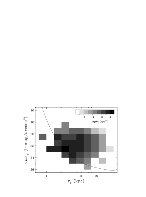
Figure 1: The space density distribution of Sb-Sdm galaxies as function of effective radius and average SB within that radius. Galaxies with exponential disk, having structural properties indicated by the line, can be seen out to 20 Mpc before dropping out of the sample.

4 Parametrization of the distributions

In this section we will define a parametrization of the bivariate distributions, as an aid to compare distributions derived from differently selected samples or to study redshift evolution. We will follow the most simple form of the Fall & Efstathiou (1980) disk galaxy formation theory to derive such a parametrization (for extended versions of the theory see e.g. van der Kruit 1987; Dalcanton et al. 1997; Mo et al. 1998; van den Bosch 1998). Galaxies form in this theory in hierarchically merging Dark Matter (DM) halos, giving rise to a distribution of DM halo masses described by the Press & Schechter (1974) theory, which formed the inspiration for the Schechter (1976) luminosity function (LF). We will use a Schechter LF to describe the luminosity dimension of our distribution function.

In the Fall & Efstathiou (1980) model, the scalesize of a galaxy is determined by its angular momentum, which is acquired by tidal toques from neighbouring DM halos in the expanding universe. The total angular momentum of the system is usually expressed in terms of the dimensionaless spin parameter (Peebles 1969)

$$\lambda=J|E|^{1/2}M_{\rm tot}^{-5/2}G^{-1},$$ (3)

with J the total angular momentum, $E$ the total energy and $M_{\rm tot}$ the total mass of the system, all of which are dominated by the DM halo. N-body simulations (e.g. Warren et al. 1992) show that the distribution of $\lambda$ values acquired from tidal torques in an expanding universe can be well be approximated by a log-normal distribution with a dispersion $\sigma_{\lambda}\sim 0.5$ in $\ln(\lambda$).

A few simplifying approximations allow us to relate each of the factors in Eq. (3) to our observed bivariate distribution parameters. A perfect exponential disk of effective size $r_{\rm e}$, mass $M_{d}$, rotating with a flat rotation curve of velocity $V_{c}$ has $J_{d}\propto M_{d}r_{\rm e}V_{c}$. We assume that the specific angular momentum of the disk is equal to the specific angular momentum of the dark halo. From the virial theorem we get $E\propto V_{c}^{2}M_{\rm tot}$. If we assume that light traces disk mass ($M_{d}\propto L)$ and that disk mass is proportional to total mass ($M_{\rm tot}\propto M_{d}$), we only need the Tully & Fisher (1977) relation ($L\propto V_{c}^{\beta}$, with $\beta\sim 3$ in the $I$-passband) to link the spin parameter $\lambda$ to our observed bivariate distribution parameters.

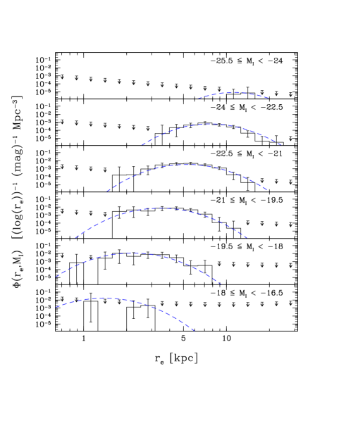
Figure 2: The space density distribution of effective scalesizes in different bins of total $I$-band luminosity as marked in the top-right of each panel. The histograms represent the data with errorbars showing the 95% confidence limits due to distance and Poisson errors. The 95% confidence upper limits were calculated using exponential disks and the survey limits determined from the photometry. The dashed line shows the bivariate distribution function described in the text.

These approximations give $\lambda\propto r_{\rm e}L^{-(2/\beta-1)}\simeq r_{\rm e}L^{-1/3}$. As $\lambda$ is expected to have a log-normal behavior, this means that, at a given luminosity, we expect the distribution of scalesizes to be log-normal, and that the peak in the $r_{\rm e}$ distribution shifts with $\sim L^{-1/3}$. This is exactly the behavior that is shown in Fig. 2, where the function over-plotted on the data shows the log-normal behavior at each luminosity bin, shifting by $L^{-1/3}$ between the luminosity bins and where the height is determined by the Schechter LF.

The function plotted is the result of the well known $\chi$-by-eye fitting method, and the detailed parameters will definitely change when a full fitting technique has been developed that takes the Poisson errors on the data points into account. For reference we list here the full bivariate function in magnitudes, and the parameter values giving a good approximation to the data:

$$\Phi(r_{\rm e},M)\,d\log r_{\rm e}\,dM = \frac{\Phi_{0}}{\sigma_{\lambda}\sqrt{2\pi}}\exp(-\frac{1}{2}[\frac{\log r_{\rm e}/r_{{\rm e}*}-0.4(M-M_{*})(2/\beta-1)}{\sigma_{\lambda}/\ln(10)}]^{2})$$

$$10^{-0.4(M-M_{*})(\alpha+1)}\,\exp(-10^{-0.4(M-M_{*})})\,d\log r_{\rm e}\,dM,$$

with the first line representing the log-normal scalesize distribution and the second line the Schechter LF in magnitudes ($M$). The $\chi$-by-eye parameters are:
$\Phi_{0}=0.002{\rm\,Mpc}^{-3}$ $\alpha=-1.25$ $\beta=3.0$  (slope Tully-Fisher relation) $M_{*}=-22.3\,I$-mag $r_{{\rm e}*}=6.7\,{\rm kpc}$ $\sigma_{\lambda}=0.3$
The width of the spin parameter distribution ($\sigma_{\lambda}$) we need is less than what is typically found in N-body simulations.

5 Discussion & conclusions

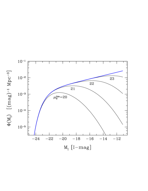
Figure 3: Luminosity functions computed by integrating the bivariate distribution function down to the indicated $I$-band central surface brightness limits. The uppermost line shows the integrated total LF.

Using our parameterization we can now estimate the effects of SB limits on determinations of LFs and on deep galaxy counts, especially in the context of (1+$z$)⁴ redshift dimming. If we were to determine the LF from a galaxy sample with low SB galaxies cut out, we would underestimate the faint end of the LF, as most low SB galaxies are also low luminosity systems. SB cuts are relevant for redshift surveys selected from shallow (photographic plate) material (resulting in implicit cuts) and for most fiber based redshift surveys which often have explicit SB cuts (e.g. the Las Campanas and Sloan Surveys). How SB cuts can effect LF determinations is shown in Fig. 3, where we have integrated our parameterization down to the indicated $I$-band central  SB.

Figure 3 suggests that the SB cuts typically present in local surveys do not dramatically effect LF determinations (using for a typical spiral $B$–$I$$\simeq$1.7), especially taking into account that most spirals have some central light enhancement due to the bulge, making detections easier. The situation changes however when we move to higher redshifts and have to take (1+$z$)⁴ cosmological redshift dimming into account. At $z$=1 our SB limit has already shifted 3 magnitudes up, and 6 magnitudes by the time we reach $z$=3. This means that even for the deepest image available at the moment –the Hubble Deep Field– the SB cut at $z$=3 (the $U$-band dropouts) runs at about 21 $I$-mag arcsec^-2 (using a K-correction of an unevolved Sb galaxy). This limit makes a considerable fraction of galaxies in Fig. 1 undetectable, if we put this local galaxy population unevolved at $z$=3.

Tully & Verheijen (1997, these proceedings) have argued that the central SB of galaxies shows a bimodal distribution, in particular when looking at $K$-band data. We do not see such bimodality, independent whether we use their proposed bimodal dust extinction correction, we use only the 200 most face-on galaxies with the smallest extinction correction, we use bulge/disk decomposed parameters or effective parameters. In the many ways we have looked at the MFB data set, we have never seen any bimodality in the SB distributions. Whether the bimodal effect is the result of the special Ursa Major cluster environent that was studied or an unlucky case of low number statistics remains to be seen.

The simple parametrization presented in this paper gives an accurate representation of the observed bivariate distributions, independently of whether one believes in hierarchical galaxy formation models or in CDM-like universes. A detailed analysis of galaxy formation in CDM-like universes paying attention to bivariate space density distributions will appear in Lacey et al. (1999).

- [1] yun, Y.-I. 1992, PhD. Thesis, The Australia National University
- [2] alcanton J. J., Spergel, D. N. & Summers, F. J. 1997, ApJ, 482, 676
- [3] e Jong, R. S. 1996, A&A, 313, 45
- [4] isney, M. J. 1976, Nature, 263, 573
- [5] isney, M. J. & Phillipps, S. 1983, MNRAS, 205, 1253
- [6] llis, R. S. 1997, ARA&A, 35, 389
- [7] all, S. M. & Efstathiou, G. 1980, MNRAS, 193, 189
- [8] elten, J. E. 1976, ApJ, 207, 700
- [9] reeman, K. C. 1970, ApJ, 160, 811
- [10] udson, M. J. & Lynden-Bell, D. 1991, MNRAS, 252, 219
- [11] mpey, C. & Bothun, G. 1997, ARA&A, 35, 267
- [12] acey, C., Cole, S., Baugh, C. & Frenk, C. S. 1999, in preparation
- [13] athewson, D. S. & Ford, V. L. 1996, ApJS, 107, 97
- [14] athewson, D. S., Ford, V. L. & Buchorn M. 1992, ApJS, 81, 413
- [15] cGaugh, S.S., Bothun, G. D. & Schombert, J. M. 1995, AJ, 110, 573
- [16] o, H. J., Mao, S. & White, S. D. M. 1998, MNRAS, 295, 319
- [17] eebles, P. J. E. 1969, ApJ, 155, 393
- [18] ress, W. H., Schechter, P. 1974, ApJ, 187, 425
- [19] chechter, P. 1976, ApJ, 203, 297
- [20] chlegel, D. J., Finkbeiner, D. P. & Davis, M. 1998, ApJ, 500, 525
- [21] odré, L. & Lahav, O. 1993, MNRAS, 260, 285
- [22] ully, R. B. & Verheijen, M. A. W. 1997, ApJ, 484, 145
- [23] an den Bosch, F. C. 1998, submitted to ApJ, astro-ph/9805113
- [24] an der Kruit, P. C. 1987, A&A, 173, 59
- [25] arren, M.S., Quinn, P. J., Salmon, J. K. & Zurek, W. H. 1992, ApJ, 399, 405
- [26] illick, J. A. et al. 1997, ApJS, 109, 333