[astro-ph/9810476] Models for large-scale structure

1 Background

This conference takes place at a time when the subject of large-scale structure is reaching a certain maturity, following a period of very rapid development. To appreciate how far we have come, it is instructive to look back nearly 20 years to the 1979 Les Houches summer school on Physical Cosmology, whose proceedings were greatly influential in their time. In 1979, there was an appreciation that galaxies displayed roughly power-law correlations (measured on small scales only), and that these would only grow by gravity if there were some significant form of initial fluctuations. However, the central problem of the origin of these initial fluctuations was scarcely mentioned. The only candidate primordial spectra mentioned were expressed in terms of the density fluctuation in a region containing $n$ particles:

$\displaystyle{{\delta n\over n}}$	$\displaystyle{{}=n^{-1/2}\quad{\rm Poisson}}$
	$\displaystyle{{}=n^{-5/6}\quad{\rm Discreteness}}$

(1)

The former comes from random placement of particles; the latter from random displacement of particles within the cells of a uniform mesh. It was known that the first gave too large an amplitude, so that the initial conditions had to be sub-random, but the particle-in-box spectrum has too small an amplitude. There was a guess that something like the Zeldovich spectrum was needed ( $\delta n/n=10^{-4}n^{-2/3}$ ), but there were no ideas on where it might come from.

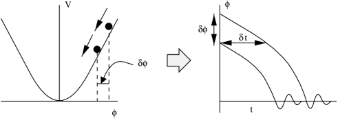
Refer to caption — Figure 1: Inflation claims that fluctuations are seeded by quantum fluctuations in the rolling of a scalar field, $\phi$ , down a potential, $V(\phi)$ .

The situation today is much more healthy; 16 years have passed since it was realized that inflation could seed these initial inhomogeneities, and a variety of models of inflationary structure formation have been analyzed in detail. Furthermore, an alternative mechanism for seeding perturbations exists through the action of topological defects. In its simplest form (see e.g. Liddle & Lyth 1993; Lyth & Riotto 1998), inflation deals with a single quantum scalar field, whose expectation value rolls down a potential (figure 1). The equation of motion is

\ddot{\phi}+3H\dot{\phi}-\nabla^{2}\phi+{dV(\phi)\over d\phi}=0.

(2)

If the potential is flat in the sense

$\displaystyle{\epsilon}$	$\displaystyle{{}\equiv{m_{\scriptscriptstyle\rm P}^{2}\over 16\pi}\,(V^{\prime}/V)^{2}\ll 1}$
$\displaystyle{\eta}$	$\displaystyle{{}\equiv{m_{\scriptscriptstyle\rm P}^{2}\over 8\pi}\,(V^{\prime\prime}/V)\ll 1}$

(3)

then vacuum-dominated ‘slow-roll’ inflationary expansion can happen, leading to the following horizon-scale amplitude for the density fluctuations:

\delta_{\scriptscriptstyle\rm H}={H^{2}\over 2\pi\dot{\phi}},

(4)

where

\displaystyle{{}H^{2}={8\pi\over 3}\,{V\over m_{\scriptscriptstyle\rm P}^{2}}}

\displaystyle{{}3H\dot{\phi}=-V^{\prime}.}

(5)

There are a few free parameters here, but the characteristic prediction of inflation is that there is a background of gravity waves. There are thus both scalar and tensor contributions to the CMB power spectrum:

C_{\ell}^{\scriptscriptstyle\rm S}\propto\ell^{n_{\scriptscriptstyle\rm S}-3},\quad\quad C_{\ell}^{\scriptscriptstyle\rm T}\propto\ell^{n_{\scriptscriptstyle\rm T}-3}

(6)

(beware: different definitions of the tensor index exist). The slopes of these spectra depend on the inflationary parameters:

$\displaystyle{{\rm scalar\ tilt}}$	$\displaystyle{{}\equiv 1-n_{\scriptscriptstyle\rm S}\equiv-{d\ln\delta^{2}_{\scriptscriptstyle\rm H}\over d\,\ln k}}$
	$\displaystyle{{}=6\epsilon-2\eta}$
$\displaystyle{{\rm tensor\ tilt}}$	$\displaystyle{{}\equiv 1-n_{\scriptscriptstyle\rm T}=2\epsilon}$

(7)

and so does the relative tensor contribution, giving the consistency equation (Starobinsky 1985; Lidsey et al. 1997):

{C_{\ell}^{\scriptscriptstyle\rm T}\over C_{\ell}^{\scriptscriptstyle\rm S}}=12\epsilon=6(1-n_{\scriptscriptstyle\rm T})

(8)

These predictions can be violated in models with several scalar fields, so inflation is a slightly soft target. Nevertheless, it would be striking if something like these relation was to be found in practice. To have both a potential mechanism for generating the inhomogeneous universe plus anything approaching a test of the theory is an astonishing achievement – whether or not the theory has anything to do with reality. In testing a theory, it is good to have an alternative in mind, but I will say little about the main class of alternatives, which are topological defects. The state of play here will be reviewed in Pen’s talk, but presently looks unpromising (e.g. Albrecht, Battye & Robinson 1998).

2 The fluctuation spectrum

2.1 The linear spectrum

The basic picture of inflationary models is therefore of a primordial power-law spectrum, written dimensionlessly as the logarithmic contribution to the fractional density variance, $\sigma^{2}$ :

\Delta^{2}(k)={d\sigma^{2}\over d\ln k}\propto k^{3+n},

(9)

where $n$ stands for $n_{\scriptscriptstyle\rm S}$ hereafter. This undergoes linear growth

\delta_{k}(a)=\delta_{k}(a_{0})\;\left[{D(a)\over D(a_{0})}\right]\;T_{k},

(10)

where the linear growth law is

D(a)=a\,g[\Omega(a)]

(11)

in the matter era, and the growth suppression for low $\Omega$ is

$\displaystyle{g(\Omega)}$	$\displaystyle{{}\simeq\Omega^{0.65}\ {\rm(open)}}$
	$\displaystyle{{}\simeq\Omega^{0.23}\ {\rm(flat)}}$

(12)

The transfer function $T_{k}$ depends on the dark-matter content as shown in figure 2. Note the baryonic oscillations in figure 2; these can be significant even in CDM-dominated models when working with high-precision data. Eisenstein & Hu (1998) are to be congratulated for their impressive persistence in finding an accurate fitting formula that describes these wiggles. This is invaluable for carrying out a search of a large parameter space.

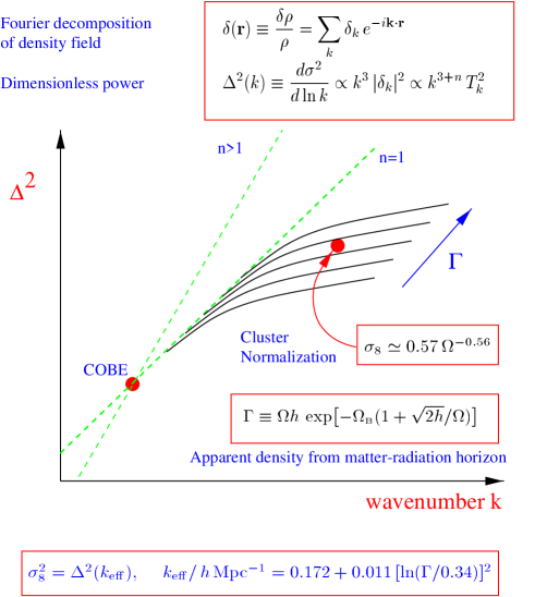
The state of the linear-theory spectrum after these modifications is illustrated in figure 3. The primordial power-law spectrum is reduced at large $k$ , by an amount that depends on both the quantity of dark matter and its nature. Generally the bend in the spectrum occurs near $1/k$ of order the horizon size at matter-radiation equality, $\propto(\Omega h^{2})^{-1}$ . For a pure CDM universe, with scale-invariant initial fluctuations ( $n=1$ ), the observed spectrum depends only on two parameters. One is the shape $\Gamma=\Omega h$ , and the other is a normalization. On the shape front, a government health warning is needed, as follows. It has been quite common to take $\Gamma$ -based fits to observations as indicating a measurement of $\Omega h$ , but there are three reasons why this may give incorrect answers: (1) The dark matter may not be CDM. An admixture of HDM will damp the spectrum more, mimicking a lower CDM density. (2) Even in a CDM-dominated universe, baryons can have a significant effect, making $\Gamma$ lower than $\Omega h$ . An approximate formula for this is given in figure 3 (Peacock & Dodds 1994; Sugiyama 1995). (3) The strongest (and most-ignored) effect is tilt: if $n\neq 1$ , then even in a pure CDM universe a $\Gamma$ -model fit to the spectrum will give a badly incorrect estimate of the density (the change in $\Omega h$ is roughly $0.3(n-1)$ ; Peacock & Dodds 1994).

2.2 Normalization

The other parameter is the normalization. This can be set at a number of points. The COBE normalization comes from large-angle CMB anisotropies, and is sensitive to the power spectrum at $k\simeq 10^{-3}\,h\,{\rm Mpc}^{-1}$ . The alternative is to set the normalization near the quasilinear scale, using the abundance of rich clusters. Many authors have tried this calculation, and there is good agreement on the answer:

\sigma_{8}\simeq(0.5-0.6)\,\Omega_{m}^{-0.6}.

(13)

(White, Efstathiou & Frenk 1993; Eke et al. 1996; Viana & Liddle 1996). In many ways, this is the most sensible normalization to use for LSS studies, since it does not rely on an extrapolation from larger scales. Within the CDM model, it is always possible to satisfy both these normalization constraints, by appropriate choice of $\Gamma$ and $n$ . This is illustrated in figure 4. Note that vacuum energy affects the answer; for reasonable values of $h$ and reasonable baryon content, flat models require $\Omega_{m}\simeq 0.3$ , whereas open models require $\Omega_{m}\simeq 0.5$ .

2.3 The velocity spectrum

Given the density spectrum, other quantities of interest can be calculated in linear theory. For example, the velocity spectrum is

{d\sigma_{v}^{2}\over d\ln k}=\left({\Omega_{m}^{0.6}H\over k}\right)^{2}\Delta^{2}(k).

(14)

A plot of this function is shown in figure 5, determined in various ways. If these determinations are all normalized according to the cluster abundance, there appears to be relatively little uncertainty in the velocity spectrum. This is not surprising, since the cluster normalization is tied to the observed abundance of a set of objects of a fixed observed velocity dispersion. Note the impressive breadth of the velocity spectrum: even modes of $600\,h^{-1}\,{\rm Mpc}$ wavelength contribute about $100\;{\rm km\,s^{-1}}$ rms to the motion of the local group. This shows why it has been hard to obtain redshift surveys of sufficient depth to obtain a convergent prediction of the local gravitational dipole. These velocity fields are responsible for the distortion of the clustering pattern in redshift space, as first clearly articulated by Kaiser (1987). For a survey that subtends a small angle (i.e. in the distant-observer approximation), a good approximation to the anisotropic redshift-space Fourier spectrum is given by the Kaiser function together with a damping term from nonlinear effects:

\delta_{k}^{s}=\delta_{k}^{r}(1+\beta\mu^{2})D(k\sigma\mu),

(15)

where $\beta=\Omega_{m}^{0.6}/b$ , $b$ being the linear bias parameter of the galaxies under study, $\mu={\bf\hat{k}\cdot\hat{r}}$ , and $D(y)\simeq(1+y^{2}/2)^{-1/2}$ , and $\sigma\simeq 350\;{\rm km\,s^{-1}}$ is the pairwise velocity dispersion of galaxies (e.g. Ballinger, Peacock & Heavens 1996). In principle, this distortion should be a robust way to determine $\Omega$ (or at least $\beta$ ); see Strauss & Willick (1995) and Hamilton (1997) for details of the practical application of these ideas.

2.4 The nonlinear spectrum

On smaller scales ( $k\mathrel{\lower 2.58334pt\hbox{$\buildrel{\textstyle>}\over{\scriptstyle\sim}$}}0.1$ ), nonlinear effects become important. These are relatively well understood so far as they affect the power spectrum of the mass (e.g. Hamilton et al. 1991; Jain, Mo & White 1995; Peacock & Dodds 1996). These methods were applied by Peacock & Dodds (1994; PD94) to estimate the linear spectrum from the observed spectrum of a number of tracers (figure 6). To within a scatter of perhaps a factor 1.5 in power, the results were consistent with a $\Gamma\simeq 0.25$ CDM model. Even though the subsequent sections will discuss some possible disagreements with the CDM models at a higher level of precision, the general existence of CDM-like curvature in the spectrum is likely to be an important clue to the nature of the dark matter.

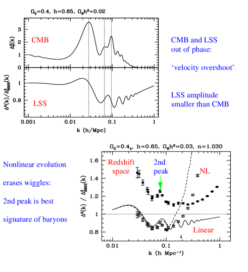
One interesting aspect of the existing spectrum determinations is that they are relatively smooth, whereas figure 2 shows that rather large oscillatory features would be expected if the universe was baryon dominated. The lack of such features is one reason for believing that the universe might be dominated by collisionless nonbaryonic matter (consistent with primordial nucleosynthesis if $\Omega_{m}\mathrel{\lower 2.58334pt\hbox{$\buildrel{\textstyle>}\over{\scriptstyle\sim}$}}0.1$ ).

Nevertheless, baryonic fluctuations in the spectrum can become significant for high-precision measurements. Figure 7 shows that order 10% modulation of the power may be expected in realistic baryonic models (Eisenstein & Hu 1998; Goldberg & Strauss 1998). Most of these features are however removed by nonlinear evolution. The highest- $k$ feature to survive is usually the second peak, which almost always lies near $k=0.05\,{\rm Mpc}^{-1}$ (no $h$ , for a change). This feature is relatively narrow, and can serve as a clear proof of the past existence of baryonic oscillations in forming the mass distribution (Meiksin, White & Peacock 1998). However, figure 7 emphasises that the easiest way of detecting the presence of baryons is likely to be through the CMB spectrum. The oscillations have a much larger ‘visibility’ there, because the small-scale CMB anisotropies come directly from the coupled radiation-baryon fluid, rather than the small-scale dark matter perturbations.

2.5 The APM spectrum

In the past few years, much attention has been attracted by the estimate of the galaxy power spectrum from the APM survey (Baugh & Efstathiou 1993, 1994; Maddox et al. 1997). The APM result was generated from a catalogue of $\sim 10^{6}$ galaxies; because it is based on a deprojection of angular clustering, it is immune to the complicating effects of redshift-space distortions.

The error estimates are derived empirically from the scatter between independent regions of the sky, and so should be realistic. If there are no undetected systematics, these error bars say that the power is very accurately determined, and this has significant implications if true. A number of authors have pointed out that the detailed spectral shape appears to be inconsistent with that of nonlinear evolution from CDM initial conditions. (e.g. Efstathiou, Sutherland & Maddox 1990; Klypin, Primack & Holtzman 1996; Peacock 1997). Perhaps the most detailed work was carried out by the VIRGO consortium, who carried out $N=256^{3}$ simulations of a number of CDM models (Jenkins et al. 1998). Their results are shown in figure 8, which gives the nonlinear power spectrum at various times (cluster normalization is chosen for $z=0$ ) and contrasts this with the APM data. The lower small panels are the scale-dependent bias that would required if the model did in fact describe the real universe, defined as

b(k)\equiv\left({\Delta^{2}_{\rm gals}(k)\over\Delta^{2}_{\rm mass}}\right)^{1/2}.

(16)

In all cases, the required bias is non-monotonic; it rises at $k\mathrel{\lower 2.58334pt\hbox{$\buildrel{\textstyle>}\over{\scriptstyle\sim}$}}5\,h^{-1}\,{\rm Mpc}$ , but also displays a bump around $k\simeq 0.1\,h^{-1}\,{\rm Mpc}$ . If real, this feature seems impossible to understand as a genuine feature of the mass power spectrum; certainly, it is not at a scale where the effects of even a large baryon fraction would be expected to act (Eisenstein et al. 1998; Meiksin, White & Peacock 1998).

An alternative way of presenting this difficulty for CDM models is shown in figure 9. Here, the methods of Peacock & Dodds (1996) have been used in an attempt to recover the empirical linear spectrum from the APM data. It is assumed that the bias is independent of scale, and that the cluster normalization applies. The results (for low and high $\Omega$ ) are contrasted with CDM models with reasonable Hubble parameters and baryon fractions. Interestingly, there is not a huge difference in shape between the CDM models. This arises because both are also consistent with COBE, and therefore have very different values of the tilt, as above. This plot should drive home the lesson that the apparent value of $\Gamma$ cannot be used as an estimate of $\Omega h$ without further, possibly fragile, assumptions. In any case, the linear spectrum that would evolve into the APM result is seen in figure 9 to differ significantly from the CDM models. The bump at $k\simeq 0.1\,h^{-1}\,{\rm Mpc}$ is apparent, as is a flattening at larger $k$ – the effective spectral index appears to approach $n=-3$ , whereas the CDM models are never this flat. A spectrum of this form would be expected with a roughly 30% admixture of massive neutrinos in a total $\Omega\simeq 1$ (Klypin et al. 1993; Pogosyan & Starobinsky 1995). This success in matching the empirical spectrum shape is a very significant attraction of the MDM model. However, there are also very serious difficulties with the idea of an MDM universe, related to the formation of high-redshift objects. MDM suffers from the same difficulties as any $\Omega=1$ model in making high-redshift massive clusters (e.g. Henry 1997). This alone may be a strong enough argument to reject the model. However, the very flatness of the high- $k$ spectrum that is attractive in terms of clustering statistics makes it difficult for MDM to assemble the observed high-redshift galaxies (e.g. Mo & Miralda-Escudé 1994; Mo & Fukugita 1996; Peacock et al. 1998). These problems are eased in a low-density model, which is probably required by the supernova Hubble diagram (Perlmutter et al 1997; Riess et al. 1998), but the MDM spectral shape is then wrong.

3 Towards an understanding of bias

The conclusions from the above discussion are either that the physics of dark matter and structure formation are more complex than in CDM models, or that the relation between galaxies and the overall matter distribution is sufficiently complicated that the effective bias is not a simple slowly-varying monotonic function of position.

3.1 Local bias

The simplest assumption is that all the complicated physical effects leading to galaxy formation depend in a causal (but nonlinear) way on the local mass density, so that we write

\rho_{\rm light}=f(\rho_{\rm mass}).

(17)

Coles (1993) showed that, under rather general assumptions, this equation would lead to an effective bias that was a monotonic function of scale. This issue was investigated in some detail by Mann, Peacock & Heavens (1998), who verified Coles’ conclusion in practice for simple few-parameter forms for $f$ , and found in all cases that the effective bias varied rather weakly with scale. The APM results thus are either inconsistent with a CDM universe, or require non-local bias.

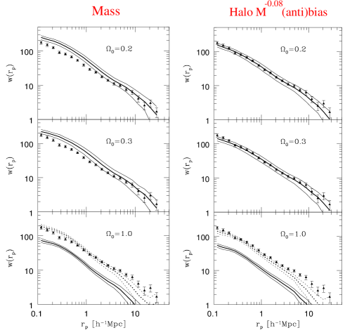
A puzzle with regard to this conclusion is provided by the work of Jing, Mo & Börner (1998). They evaluated the projected real-space correlations for the LCRS survey (see figure 10). This statistic also fails to match the prediction of CDM models, but this can be amended by introducing a simple antibias scheme, in which galaxy formation is suppressed in the most massive haloes. This scheme should in practice be very similar to the Mann, Peacock & Heavens recipe of a simple weighting of particles as a function of the local density; indeed, the main effect is a change of amplitude, rather than shape of the correlations. The puzzle is this: if the APM power spectrum is used to predict the projected correlation function, the result agrees almost exactly with the LCRS. Either projected correlations are a rather insensitive statistic, or perhaps the Baugh & Efstathiou deconvolution procedure used to get $P(k)$ has exaggerated the significance of features in the spectrum. The LCRS results are one reason for treating the apparent conflict between APM and CDM with caution.

3.2 High-order correlations

A further piece of evidence concerning bias comes from the higher-order correlations of the density field, which are most conveniently described via the hierarchical moments:

S_{J}\equiv{\langle\delta^{J}\rangle/[\langle\delta^{2}\rangle]^{J-1}}.

(18)

These are defined so that, for gravitationally-driven growth of fluctuations, the $S_{J}$ are dimensionless numbers that can be calculated in perturbation theory. For example, if the density field is smoothed with a spherical top-hat window, the third moment for a Gaussian field should be

S_{3}={34\over 7}-(3+n)

(19)

(Bernardeau 1994). In the presence of pure linear bias of the density field, $\delta_{\rm gals}=b\delta_{\rm mass}$ , $S_{J}\rightarrow b^{2-J}S_{J}$ , so there might seem to be an interesting test here both of Gaussianity and of whether light traces mass. In practice, Gaztañaga & Frieman (1994) found that higher-order results from (again) the APM catalogue were in remarkably good agreement with the simplest unbiased Gaussian predictions. However, the interpretation of this result needs care: linear density bias is unphysical, in that it can yield $\delta<-1$ . Gravitational evolution causes increasing skewness to develop because this is the only way in which a large second moment $\langle\delta^{2}\rangle\gg 1$ can coexist with the $\delta>-1$ constraint. Any bias scheme that has the effect of increasing $\langle\delta_{\rm gals}^{2}\rangle$ relative to $\langle\delta_{\rm mass}^{2}\rangle$ is almost certain to increase the skewness also. The higher-order results are thus quite a significant limit on non-Gaussianity, but do not strongly constrain bias.

3.3 Halo correlations

In reality, bias is unlikely to be completely causal, and this has led some workers to explore stochastic bias models, in which

\rho_{\rm light}=f(\rho_{\rm mass})+\epsilon,

(20)

where $\epsilon$ is a random field that is uncorrelated with the mass density (Pen 1998; Dekel & Lahav 1998). Although truly stochastic effects are possible in galaxy formation, a relation of the above form is expected when the galaxy and mass densities are filtered on some scale (as they always are, in practice). Just averaging a galaxy density that is a nonlinear function of the mass will lead to some scatter when comparing with the averaged mass field; a scatter will also arise when the relation between mass and light is non-local, however, and this may be the dominant effect. The simplest and most important example of non-locality in the galaxy-formation process is to recognize that galaxies will generally form where there are galaxy-scale haloes of dark matter. In the past, it was generally believed that dissipative processes were critically involved in galaxy formation, since pure collisionless evolution would lead to the destruction of galaxy-scale haloes when they are absorbed into the creation of a larger-scale nonlinear system such as a group or cluster. However, it turns out that this overmerging problem was only an artefact of inadequate resolution. When a simulation is carried out with $\sim 10^{6}$ particles in a rich cluster, the cores of galaxy-scale haloes can still be identified after many crossing times (Ghigna et al. 1997). This is a very important result, since it holds out the hope that many of the issues concerning where galaxies form in the cosmic density field can be settled within the domain of collisionless simulations. Dissipative physics will still be needed to understand in detail the star-formation history within a galaxy-scale halo. Nevertheless, the idea that there may be a one-to-one correspondence between galaxies and galaxy-scale dark-matter haloes is clearly an enormous simplification – and one that increases the chance of making robust predictions of the statistical properties of the galaxy population. Another piece of work which also emphasises the survival of galaxy-scale haloes is Klypin et al. (1997; see also Kravtsov’s talk at this meeting). Rather than looking only at a single cluster, Klypin et al. attempt to find galaxy haloes within a random cosmological volume. Their results are shown in figure 11, where the correlation function for the mass in a $\Lambda$ CDM simulation is contrasted with the correlation function for the haloes. The mass $\xi(r)$ shows the familiar form: the sharp quasilinear rise between $\xi\simeq 10$ and 300, followed by the flattening associated with virialization. By contrast, the halo correlation functions are much closer to single power laws: they are antibiased at $\xi\simeq 100$ , but positively biased for $\xi\mathrel{\lower 2.58334pt\hbox{$\buildrel{\textstyle>}\over{\scriptstyle\sim}$}}1000$ . These are qualitatively the trends that are required in order to reconcile the APM data with CDM models, so this is clearly a result of great potential significance. Future work should improve the precision of the results and allow the simulation boxes to be made larger (they are presently uncomfortably small). However, if the result holds up, we will be no nearer an understanding of what is going on. A simple result like power-law correlations demands to be explained in a more intuitive manner. If the result turns out to be inevitable on some general grounds, then this may be bad news for the idea of large-scale-structure studies as a diagnostic tool – it is possible that the galaxy correlations may turn out to be less sensitive to the underlying linear power spectrum than the mass correlations are.

4 Clustering at high redshifts

A longstanding ambition has been to remove some of the uncertainties concerning the generation of large-scale structure by observing the growth of clustering with time. After a number of years of ambiguous results from angular clustering of faint galaxies, this has at last proved possible by using deep redshift surveys. Perhaps the first convincing measurement of clustering evolution came from the CFRS (Le Fèvre et al. 1996), which indicated evolution in the sense that $\xi$ at a given comoving separation was a factor of about four smaller at $z=1$ than it is today. Evolution in the same sense (but somewhat less strong) has been found by the CNOC2 team (Carlberg et al. 1998). These results appear to prove that clustering does indeed grow by gravity, but this idea looks less convincingly demonstrated when the results from clustering at higher redshifts are considered. It is remarkable that samples at $z\simeq 3.5$ are now as large as those at $0.5\mathrel{\lower 2.58334pt\hbox{$\buildrel{\textstyle<}\over{\scriptstyle\sim}$}}z\mathrel{\lower 2.58334pt\hbox{$\buildrel{\textstyle<}\over{\scriptstyle\sim}$}}1$ were only two years ago; this shows how efficient the Lyman-break selection technique has been. At this highest redshift, we have the remarkable result that the comoving correlation strength appears to be very close to that measured today (Steidel et al. 1998; Adelberger et al. 1998). In other words, any downward evolution in $\xi$ between $z=0$ and $z=1$ must be reversed between $z=1$ and $z=3.5$ , so that $\xi(z)$ has a minimum. Alternatively, if we believe that clustering of the mass grows monotonically according to gravitational instability, then clustering at $z=3.5$ must be very strongly biased. Steidel et al. (1998) obtain a minimum bias of 6, with a preferred value of 8, assuming $\Omega=1$ . It is easy to translate to other models, since we observe cell variances $\sigma^{2}_{\rm cell}$ directly, where the cell has a given angular width and depth in redshift. For low $\Omega$ models, the cell volume will increase by a factor $[S_{k}^{2}(r)\,dr]/[S_{k}^{2}(r_{1})\,dr_{1}]$ ; comparing with present-day fluctuations on this larger scale will tend to increase the bias. However, for low $\Omega$ , two other effects increase the predicted density fluctuation at $z=3$ : the cluster constraint increases the present-day fluctuation by a factor $\Omega^{-0.56}$ , and the growth between redshift 3 and the present will be less than a factor of 4. Applying these corrections gives

{b(\Omega=0.3)\over b(\Omega=1)}=\left\{{0.42\ ({\rm open})\atop 0.60\ \hbox to0.0pt{({\rm flat})\hss}\phantom{({\rm open})}}\right.,

(21)

which suggests an approximate scaling as $b\propto\Omega^{0.72}$ (open) or $\Omega^{0.42}$ (flat). Strong bias is needed at $z=3$ for all reasonable values of $\Omega$ . The standard explanation for this effect is high-peak bias, which is bound to operate if the high-redshift galaxies are rare, newly-forming systems. The linear bias parameter depends on the rareness of the fluctuation and the rms of the underlying field as

b=1+{\nu^{2}-1\over\nu\sigma}=1+{\nu^{2}-1\over\delta_{c}}

(22)

(Kaiser 1984; Cole & Kaiser 1989; Mo & White 1996 – but see also Jing 1998), where $\nu=\delta_{c}/\sigma$ , and $\sigma^{2}$ is the fractional mass variance at the redshift of interest. A bias at the observed level is therefore to be expected, provided the Lyman-break galaxies are moderately massive systems, with circular velocities $V\simeq 150\;{\rm km\,s^{-1}}$ (e.g. Bagla 1998a, b; Peacock et al. 1998). The minimum in $\xi$ makes sense since we observe something proportional to $(b\sigma)^{2}$ ; $b$ is constant for large $\sigma$ , but scales as $\sigma^{-2}$ for small $\sigma$ ; the observed clustering therefore has a minimum at the redshift where $\sigma\simeq 1$ . In order to turn this plausibility argument into a proof, two tests should be carried out. First, the circular velocities of Lyman-break galaxies need to be measured; second, even larger and more detailed redshift surveys need to be carried out at $z\simeq 3$ , in order to verify that the structures causing $\xi(r)$ have the same topological character of voids and filaments as seen in local large-scale structure. If these criteria are satisfied, then we can claim to have some understanding of the growth of structure, and the existing clustering results may be used as a test of models.

5 Conclusions

It should be clear from this talk that large-scale structure has advanced enormously as a field in the past two decades. Many of our long-standing ambitions have been realised; in some cases, much faster than we might have expected. Of course, solutions for old problems generate new difficulties. Although we now have good measurements of the clustering spectrum and its evolution, it is less clear that the placement of galaxies with respect to the mass is simple enough to use these results as direct statistics with which to test theories. A fairly safe bet is that one of the major results from new large surveys such as 2dF and Sloan will be a heightened appreciation of the subtleties of this problem. Nevertheless, we should not be depressed that problems remain. Observationally, we are moving from an era of 20% – 50% accuracy in measures of large-scale structure to a future of pinpoint precision. This maturing of the subject will demand more careful analysis and rejection of some of our existing tools and habits of working. The prize for rising to this challenge will be the ability to claim a real understanding of the origin of structure in the universe. We are not there yet, but there is a real prospect that the next 5–10 years may see this remarkable goal achieved.

References

Adelberger K., Steidel C., Giavalisco M., Dickinson M., Pettini M., Kellogg M., 1998, ApJ, 505, 18
Albrecht A., Battye R.A., Robinson J., 1997, astro-ph/9711121
Bagla J.S., 1998b, MNRAS, 299, 417
Bagla J.S., 1998a, MNRAS, 297, 251
Ballinger W.E., Peacock J.A., Heavens A.F., 1996, MNRAS, 282, 877
Baugh C.M., Efstathiou G., 1993, MNRAS, 265, 145
Baugh C.M., Efstathiou G., 1994, MNRAS, 267, 323
Bernardeau F., 1994, ApJ, 433, 1
Carlberg R.G. et al., 1998, astro-ph/9805131
Cole S., Kaiser N., 1989, MNRAS, 237, 1127
Coles P., 1993, MNRAS, 262, 1065
Dekel A., Lahav O., 1998, astro-ph/9806193
Efstathiou G., Sutherland W., Maddox S.J., 1990, Nature, 348, 705
Eisenstein D.J., Hu W., 1998, ApJ, 496, 605
Eisenstein D.J., Hu W., Silk J., Szalay A.S., 1998, ApJ, 494, L1
Eke V.R., Cole S., Frenk C.S., 1996, MNRAS, 282, 263
Gaztañaga E., Frieman J.A., 1994, ApJ, 437, 13
Ghigna S., Moore B., Governato F., Lake G., Quinn T., Stadel J., 1998, MNRAS, 300, 146
Goldberg D.M., Strauss M.A., 1998, ApJ, 495, 29
Hamilton A.J.S., Kumar P., Lu E., Matthews A., 1991, ApJ, 374, L1
Hamilton A.J.S., 1997, astro-ph/9708102
Henry J.P., 1997, ApJ, 489, L1
Jain B., Mo H.J., White S.D.M., 1995, MNRAS, 276, L25
Jenkins A., Frenk C.S., Pearce F.R., Thomas P.A., Colberg J.M., White S.D.M., Couchman H.M.P., Peacock J.A., Efstathiou G., Nelson A.H., 1998, ApJ, 499, 20
Jing Y.P., 1998, ApJ, 503, L9
Jing Y.P., Mo H.J., Börner G., 1998, ApJ, 494, 1
Kaiser N., 1984, ApJ, 284, L9
Kaiser N., 1987, MNRAS, 227, 1
Klypin A., Holtzman J., Primack J., Regős E., 1993, ApJ, 416, 1
Klypin A., Primack J., Holtzman J., 1996, ApJ, 466, 13
Klypin A., Gottloeber S., Kravtsov A.V., Khokhlov A.M., 1997, astro-ph/9708191
Le Fèvre O., et al., 1996. ApJ, 461, 534
Liddle A.R., Lyth D., 1993, Phys. Reports, 231, 1
Lidsey J.E. et al., 1997, Rev. Mod. Phys., 69, 373
Lyth D.H., Riotto A., 1998, hep-ph/9807278
Maddox S. Efstathiou G., Sutherland W.J., 1996, MNRAS, 283, 1227
Mann R.G., Peacock J.A., Heavens A.F., 1998, MNRAS, 293, 209
Meiksin A.A., White M., Peacock J.A., MNRAS, submitted
Mo H.J., Miralda-Escudé J., 1994, ApJ, 430, L25
Mo H.J., Fukugita M., 1996, ApJ, 467, L9
Mo H.J., White S.D.M., 1996, MNRAS, 282, 1096
Peacock J.A., Dodds S.J., 1994, MNRAS, 267, 1020
Peacock J.A., Dodds S.J., 1996, MNRAS, 280, L19
Peacock J.A., 1997, MNRAS, 284, 885
Peacock J.A., Jimenez R., Dunlop J.S., Waddington I., Spinrad H., Stern D., Dey A., Windhorst R.A., 1998, MNRAS, 296, 1089
Pen, W.-L., 1998, ApJ, 504, 601
Perlmutter S. et al., 1997, ApJ, 483, 565
Pogosyan D.Y., Starobinsky A.A., 1995, ApJ, 447, 465
Riess A.G. et al., 1998, A.J., 116, 1009
Starobinsky A.A., 1985, Sov. Astr. Lett., 11, 133
Steidel C.C., Adelberger K.L., Dickinson M., Giavalisco M., Pettini M., Kellogg M., 1998, ApJ, 492, 428
Strauss M.A., Willick J.A., 1995, Physics Reports, 261, 271
Sugiyama N., 1995, ApJS, 100, 281
Viana P.T., Liddle A.R., 1996, MNRAS, 281, 323
White S.D.M., Efstathiou G., Frenk C.S., 1993, MNRAS, 262, 1023

Models for large-scale structure

Abstract