THE MAGNETIC ASSOCIATION OF CORONAL BRIGHT POINTS

Abstract

Several coronal bright points identified in a quiet region of the Sun from SOHO/EIT Fe XII images are found to have a time evolution from birth to decay which is extremely well correlated with the rise and fall of magnetic flux as determined from photospheric magnetograms made with the SOHO/MDI instrument. Radiative losses of the bright points are found to be much less than conductive losses but the sum of the two is comparable with the available energy of the associated magnetic field. Several small ‘network flares’ occur during the lifetimes of these bright points, emphasizing the strong connection of such events with the magnetic field.

1 Introduction

New high-resolution observations from the Solar and Heliospheric Observatory (SOHO) are enabling comparisons to be made of extreme ultraviolet (EUV) features in the solar atmosphere with the photospheric magnetic field. The association of coronal X-ray bright points (XBPs) with ephemeral bipolar magnetic regions is well known (Golub et al., (1977)), but the connection can now be more satisfactorily examined with data from the Michelson Doppler Imager (MDI) on SOHO (Scherrer et al., (1995)), which forms photospheric magnetograms with spatial resolution of 1.2^′′ at a frequency of approximately one per 3 s, as well as coronal images from the SOHO Extreme Ultraviolet Imaging Telescope (EIT) (Delaboudinière et al., (1995)) and the Soft X-ray Telescope (SXT) (Tsuneta, (1991)) on the Yohkoh spacecraft. Some results already discussed (Schrijver et al., (1997); Schrijver et al., (1998)) show that the photospheric magnetic field outside of active regions is in a continuous state of replenishment, with flux emerging from below and disappearing when collisions of flux concentrations with opposite polarity occur. It is evident from MDI magnetograms how flux concentrations break into fragments which then collide with other flux concentrations of opposite polarity (resulting in partial or total flux cancellation) or the same polarity (resulting in newly merged concentrations).

The results reported here are from a study of coronal bright points, identified from EIT Fe XII and Yohkoh X-ray images, and the photospheric magnetic field from MDI data, over a period of two days when solar activity was at an extremely low level. We examine the connection between photospheric magnetic field flux and the EUV flux and the occurrence of several small ‘network flares’. The estimated energy of the magnetic field is compared with the energy that the coronal bright point plasma loses by conduction and radiation.

2 Observations

The period chosen for this study was 1997 July 31 (00:00 U.T.) to August 2 (00:00 U.T.) when solar activity was at almost the lowest level during the recent solar minimum. Two small active regions (NOAA 8064 and 8066) were on the disk but showed no flaring activity, while the X-ray emission as detected by the GOES monitoring satellites showed only tiny fluctuations with steady component at the A1 ($1\times 10^{-8}$ W m^-2) level. The Soft X-ray Telescope (SXT) on Yohkoh performed $128\times 128$ pixel partial frame rasters, covering the quiet region at the center of the Sun, with half-resolution, i.e. with pixel size 4.9^′′, so with a field of view $10^{\prime}\times 10^{\prime}$. The total observing time of this region was 4.5 hours with a mean cadence of 25 s. For most of the period, the thin aluminum (Al 0.1) and aluminum/magnesium (Al/Mg) filters were used, with bandpasses in the 3–20 Å range.

The EIT instrument regularly obtains full-Sun images at four different wavelengths, but those of interest here are made at 9 to 20 minute intervals in a 170–220 Å-wide band centered on a strong Fe XII line at 195 Å, which has peak emissivity at electron temperature $T_{e}\sim 1.4$ MK. We also used MDI full-disk images averaged over five-minute intervals which are available every 90 minutes approximately.

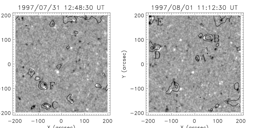
Figure 1: Two magnetograms of a quiet-Sun region at Sun center taken about a day apart, during the period discussed in the paper. North is at the top, east on the left. White areas correspond to positive polarity, black to negative. Contours show Fe XII emission and correspond to levels of 120 and 200 DN/pixel/s. Letters A to F denote the bright points discussed in the text.

We co-aligned the images for study by allowing for differential rotation using the procedure of Howard et al. (1990), with time set at 00:00 U.T. on 1997 August 1. Regions of bright Fe XII emission and significant magnetic field change over periods of only a few hours. We show representative images from MDI (gray-scale) and EIT Fe XII emission (black contours) in Fig. 1. Each image is a square with side 400^′′ (approximately $290\,000$ km).

3 Analysis and Discussion

3.1 Magnetic Flux and Coronal Emission

Inspection of the MDI magnetograms shows many changes in the form of flux-concentration motions which give rise to diverging and converging bipoles and disappearance of magnetic elements. Coronal bright points are observed in SXT and EIT images, with lifetimes of several hours, which are co-spatial and simultaneous with changes in the MDI magnetograms, normally in the form of either diverging or converging bipoles. We studied six such regions, marked A to F in Fig. 1.

Using the measured magnetic field strengths in the MDI magnetograms, we calculated values of magnetic flux $\Phi$ (in Mx), equal to $\int\mid B_{l}\mid dS$ where $B_{l}$ is the magnetic field strength (in Gauss) measured along the line of sight and the integral is over a small rectangular area $\int dS$ which includes the region of significant Fe XII emission. This area varied according to the region (e.g. for region A it was $36^{\prime\prime}\times 30^{\prime\prime}$ and for region B $40^{\prime\prime}\times 25^{\prime\prime}$).

We found that the Fe XII emission within each area is highly time-correlated with $\Phi$, with rise and fall accomplished in a period of about a day. This is illustrated for the case of region A in Fig. 2. Here, the general rise and fall of the Fe XII emission and $\Phi$ are nearly coincident (note that the $\Phi$ curve is much less frequently sampled) as are the two peaks at approximately 00:00 U.T. and 08:00 U.T. on August 1. The Fe XII flux for the six regions is almost proportional to $\Phi$. Best-fit power-law relations between the two, of the form $F_{\rm Fe\,XII}=F_{0}\ (\Phi/10^{18})^{\gamma}$ DN s^-1, showed that $\gamma$ was close to unity. (One DN or digital number corresponds roughly to 18 electrons for the EIT instrument, and to 100 electrons for the Yohkoh SXT.) Values of $F_{0}$ and $\gamma$ are given in Table 1. The X-ray signal from the SXT instrument for this period is always very weak, but it is clear from the light-curves of each region that the emission is also correlated with the rise and fall of $\Phi$ (top panel of Fig. 2). A similar relation was found for global, total magnetic flux (from vector magnetograms) and global X-ray luminosity by Fisher et al. (1998); their value of $\gamma$ (1.19) is similar to those in Table 1.

To estimate the energy contained by the magnetic field, we took the field configuration to be in the form of a semicircular loop with footpoints marked by the two monopoles. The loop is assumed to have uniform cross section with area equal to the mean of the two monopole areas. This gives a volume $V^{\prime}$ and a magnetic energy $V^{\prime}B_{l}^{2}/8\pi$. We found that, at the time when the local value of $\Phi_{l}$ reaches its maximum, the energy over the assumed loop volume was $\sim 10^{29}$ erg for all analyzed regions.

From the measured SXT flux in the Al 0.1 and Al/Mg filters we can calculate temperatures $T_{e}$ and emission measures $EM=\int N_{e}^{2}dV$ (cm^-3) with $N_{e}$ the electron density of each bright point, following Tsuneta et al. (1991). These are well determined for regions B, C and F, but not for the remaining bright points because of the weak SXT signal. Plasma temperatures do not change significantly during the period of SXT observation except for region C, where the temperature decreased from 1.7 MK to 0.8 MK. From SXT images we estimated the volume $V$ of each bright point making the simple assumption that emitting volume was either spherical or ellipsoidal, depending on its appearance. (Note that this volume is in general larger than volume $V^{\prime}$ mentioned above.) We then calculated the plasma thermal energy $3N_{e}kT_{e}V$. These values, listed in Table 1, are about two orders of magnitude less than the energy contained by the magnetic field.

Table 1 also compares bright point energy losses during their lifetime due to radiation and thermal conduction. Because SXT data cover only 10% of the period of analysis and suffer discontinuities due to orbital nights, we calculated radiative losses by integrating the EIT Fe XII light curve scaled to the SXT fluxes. Typically, the radiative energy loss is $\sim 10^{28}$ erg during the bright point lifetime, i.e. only 10% of the magnetic energy. For conductive energy losses we assumed Spitzer conductivity, i.e. that energy is conducted down to the chromosphere along field lines which are taken to have simple geometry. As can be seen, conductive energy losses are at least a factor ten more effective than radiative losses and the total energy losses are within a factor of 2 of the calculated magnetic energy.

3.2 Network Flaring

Many short-lived enhancements can be identified in the EIT Fe XII flux, often consisting of a single point (the time cadence of these observations is 20 minutes). Such an enhancement occurs, e.g., in the general rise of the emission of region A at around 22:13 U.T. on July 31 (see Fig. 2). Similar enhancements were found by Krucker & Benz (1998) in EIT data. We examined the SXT flux for the appropriate interval for X-ray counterparts of these flare-like events. The signal is weak but we found at least six significant enhancements: Fig. 3 shows light curves of three of them. The time development is not always fully observed because of the periodic night-time intervals of Yohkoh, but it is evident that there is a large variety of rise and decay times. The X-ray equivalent of the Fe XII enhancement in region B, for example, is a very impulsive event with total duration of only five minutes, whereas the event whose rise phase only is observed from region C at about 21:30 U.T. on July 31 is clearly much more gradual.

Using the ratio of fluxes in the SXT Al 0.1 and Al/Mg filters, we derived peak temperatures and emission measures. These values, which are corrected by subtraction of pre-event emission, are listed in Table 2. The temperatures are between 1 MK and 2 MK while the emission measures are approximately $10^{45}$ cm^-3, or about $10^{-5}$ times smaller than a very large solar flare. As before, the emitting volumes were estimated from the SXT images, enabling the total thermal energies $E_{\rm th}$ to be determined. These and the values of $N_{e}$ are given in Table 2. Also, total emitted energies are given, estimated from the temperature and the radiative loss data of Mewe et al. (1985).

These tiny events are very likely the ‘network flares’ noted by Krucker et al. (1997) from SXT and centimeter-wavelength radio data. The flares discussed by them have very similar characteristics to those listed in Table 2, and may be classed as micro-flares in view of their thermal energies and emission measures compared with very large solar flares. What we have established here is that they are spatially coincident with magnetic features identifiable from the MDI magnetograms. They occur during various stages in the time evolution of their associated coronal bright points, from development to decay. There is also no apparent preference for the type of magnetic activity, with network flares being emitted by emerging flux regions like F as well as cancelling flux regions like C. It appears, then, that network flares have very similar properties to conventional, active-region flares (association with bipolar magnetic field, large variety of time developments in soft X-rays, impulsive microwave burst preceding the soft X-ray emission); only their size and location (quiet-Sun regions) distinguish them.

The frequency of the flares averaged over the whole solar surface can be estimated from our data, but with only 6 events our result will be subject to at least a 40% uncertainty. The six flares occurred during 4.5 hours of effective SXT observation time over an area of $400^{\prime\prime}\times 400^{\prime\prime}$, which corresponds to about $2300\pm 1000$ per day over the whole Sun. The average thermal energy of our flares is $7\times 10^{26}$ erg (Table 2), so the energy rate requirement is $2\times 10^{25}$ erg s^-1, which is exactly the same as the corresponding rate of Krucker et al. (1997). Because these events were identified by eye inspection, the above values should be treated as lower limits only.

4 Summary and conclusions

We have established that the magnetic flux $\Phi$ as determined from the photospheric magnetic field is highly time-correlated with the Fe XII ultraviolet line emission from the six coronal bright points studied here. There appears to be a good time correlation also with the X-ray flux though the X-ray emission is in all cases very weak. For three of the bright points for which temperature and emission measure are reasonably well determined, the amount of magnetic energy, calculated from the simple model loop indicated in section 3.1, is within a factor of two of the total energy loss of the plasma over its lifetime. In view of the uncertainties of the magnetic energy calculation and the determination of the energy losses, we consider that the difference between magnetic energy and total energy loss is insignificant, i.e. that the magnetic energy supplies practically all the energy lost by the bright point plasma.

This result may be considered in the context of the ideas developed by Falconer et al. (1997, 1998) from observations that coronal features can be categorized into low-lying, “core” loops and overlying, extended features, each crossing neutral lines and possibly sheared. Core-field activity is found to drive up to apparently 10 times more heating in the surrounding extended loop configurations. They also found that magnetic flux cancellation in the core region occurs as a coronal heating agent in addition to the observed field shear, true for both active regions and the quiet Sun. Thus, this core field activity possibly drives most of the heating of the quiet-Sun corona.

Our findings would not seem to support Falconer et al. if indeed the amount of magnetic energy calculated from photospheric magnetograms is equal to that lost by a coronal bright point in its lifetime by radiation and conduction. Although there are factor-of-two uncertainties in the values of Table 1, it appears that there is very little energy available from the magnetic field over that needed to maintain the energy losses of the core configuration assuming this is identifiable as the coronal bright point.

We are, however, hesitant in asserting that there is a contradiction with the findings of Falconer et al. (1997, 1998). The energy losses of the coronal bright points given in Table 1 are almost entirely due to conduction, and they are calculated on the assumption of Spitzer conductivity acting along the field lines with simple geometry. However, the field geometry may be far from simple, as shown by the presence of flare loop-top sources (Feldman et al., 1994), and may involve turbulent fields as in the model of Jakimiec et al. (1998). If complex field geometries applied to coronal bright points, the energy loss would be much less than calculated in section 3.1. A large fraction of the magnetic energy would then be available for heating of the extended loop structures of the general corona, compatible with Falconer et al. (1998).

Finally, we note the presence of several short-lived X-ray enhancements which are like very small flares and seem to be a common feature of coronal bright points. A lower limit to the energy rate over the whole Sun is very roughly $2\times 10^{25}$ erg s^-1.

Table 1: Power-law parameters for relation between observed EIT Fe XII flux (DN s^-1) and local magnetic flux $\Phi_{l}$, $F_{\rm Fe\,XII}=F_{0}\ (\Phi/10^{18})^{\gamma}$ and comparison energies of coronal bright points (time of maximum development).

Region	$F_{0}$	$\gamma$	Thermal energy	Radiative energy	Conductive energy	Magnetic energy
			[ergs]	loss (in 1–300 Å) [ergs]	loss [ergs]	[ergs]
A	42	1.20				$1.0\times 10^{29}$
B	38	1.04	$3.8\times 10^{26}$	$5.6\times 10^{27}$	$>4\times 10^{28}$	$1.4\times 10^{29}$
C	160	0.72	$9.5\times 10^{26}$	$1.1\times 10^{28}$	$1.4\times 10^{29}$	$7.9\times 10^{28}$
D	41	1.07				$>2\times 10^{28}$
E	0.4	1.95				$1.7\times 10^{29}$
F	86	0.90	$2.0\times 10^{27}$	$6.0\times 10^{27}$	$2.6\times 10^{29}$	$2.4\times 10^{29}$

Table 2: Physical parameters of network flares from SXT observations

Region	Time	$T_{e}$	$EM$	$N_{e}$	$E_{\rm th}$	Emitted energy
	(Date/U.T.)	[MK]	[cm-3]	[cm-3]	[erg]	(in 1-300 Å) [erg]
B	1/08:42	1.9	$1.6\times 10^{45}$	$1.6\times 10^{9}$	$7.7\times 10^{26}$	$1.3\times 10^{25}$
C	31/21:45	2.2	$3.0\times 10^{44}$	$1.3\times 10^{9}$	$2.2\times 10^{26}$	$>1\times 10^{25}$
C	1/00:37	2.4	$2.5\times 10^{45}$	$2.0\times 10^{9}$	$1.3\times 10^{27}$	$5.5\times 10^{25}$
D	1/05:27	1.7	$1.2\times 10^{45}$	$1.8\times 10^{9}$	$4.6\times 10^{26}$	$5.0\times 10^{25}$
E	1/08:43	1.7	$2.7\times 10^{45}$	$2.7\times 10^{9}$	$6.9\times 10^{26}$	$6.3\times 10^{25}$
F	31/23:25	4.9	$8.4\times 10^{43}$	$5.9\times 10^{8}$	$2.9\times 10^{26}$	$1.0\times 10^{24}$

Figure 2: The SXT Al 0.1 (top) and EIT Fe XII (middle) light-curves of the coronal bright point A, together with (bottom) time variations in the local magnetic flux $\Phi$ from the MDI instrument.

Figure 3: Light-curves of three network flares observed by the Yohkoh SXT instrument in the Al 0.1 filter. The locations of the flares are identified by the regions shown in Fig. 1.

References

- Delaboudinière et al., (1995) Delaboudinière, J.-P. et al. 1995, Sol. Phys., 162, 291
- Falconer et al., (1997) Falconer, D. A., Moore, R. L., Porter, J. G., Gary, G. A., & Shimizu, T. 1997, ApJ, 482, 519
- Falconer et al., (1998) Falconer, D. A., Moore, R. L., Porter, J. G., & Hathaway, D. H. 1998, ApJ, 501, 386
- Feldman et al., (1994) Feldman, U., Hiei, E., Phillips, K. J. H., Brown, C. M., & Lang, J., 1994, ApJ, 421, 843
- Fisher et al., (1998) Fisher, G. H., Longcope, D. W., Metcalf, T. W., & Pevtsov, A. A. 1998, ApJ, submitted
- Golub et al., (1977) Golub, L., Krieger, A. S., Harvey, J. W., & Vaiana, G. S. 1977, Sol. Phys., 53, 111
- Howard, (1990) Howard, R.F., Harvey, J.W., & Forgach, S. 1990, Sol. Phys. 130, 295
- Jakimiec et al., (1998) Jakimiec, J., Tomczak, M., Falewicz, R., Phillips, K. J. H., & Fludra, A., 1998. A&A, 334, 1112
- Krucker et al., (1997) Krucker, S., Benz, A. O., Bastian, T. S., & Acton, L. W. 1997, ApJ, 488, 499
- Krucker & Benz, (1998) Krucker, S., & Benz, A. O. 1998, ApJ, 501, L213
- Mewe et al., (1985) Mewe, R., Gronenschild, E. H. B. M., & van den Oord, G. H. J. 1985, A&AS, 62, 197
- Scherrer et al., (1995) Scherrer, P. H. et al. 1995, Sol. Phys., 162, 129
- Schrijver et al., (1997) Schrijver, C. J., Title, A. M., van Ballegooijen, A. A., Hagenaar, H. J., & Shine, R. A. 1997,ApJ, 487, 424
- Schrijver et al., (1998) Schrijver, C. J. et al. 1998, Nature, 394, 152
- Tsuneta, (1991) Tsuneta, S. 1991, Sol. Phys., 136, 37