[

Cosmic string loops and large-scale structure

Abstract

We investigate the contribution made by small loops from a cosmic string network as seeds for large-scale structure formation. We show that cosmic string loops are highly correlated with the long-string network on large scales and therefore contribute significantly to the power spectrum of density perturbations if the average loop lifetime is comparable to or above one Hubble time. This effect further improves the large-scale bias problem previously identified in earlier studies of cosmic string models.

]

A Introduction

Quantitative predictions for the large-scale structure induced by cosmic strings have taken some time to crystallise as the understanding of cosmic string physics has improved [1]. In particular, the role of small loops produced by the string network has evolved from a potential one-to-one correspondence between loops and cosmological objects [2] through to a completely subsidiary role relative to the wakes swept out by long strings [3]. This dethronement of loops was a result of numerical studies which showed that the average loop size $\bar{\ell}=\alpha t$ was much smaller than the horizon, $\bar{\ell}<\!<d_{\rm H}$ [4, 5]; they might even be as small as the lengthscale set by gravitational backreaction $\alpha\sim 10^{-4}$, a value appropriate for GUT-scale strings [1]. Add the high ballistic loop velocities observed $\bar{v}\approx c/\sqrt{2}$ and it was not surprising that these tiny loops have been assumed to be more or less uniformly distributed and hence a negligible source relative to the long string network [6]. Nevertheless, small loops always make up a significant fraction of the total string energy density at any one time and, as we demonstrate here, loop-induced inhomogeneities are considerable if their lifetime is not much smaller than the Hubble time. By properly incorporating these loop perturbations, we show that their contribution relative to the long string wakes is almost comparable and also highly correlated with these wakes.

The context for this work is a major programme of structure formation simulations seeded by high resolution cosmic string networks with very large dynamic ranges [7, 8, 9]. This work demonstrated that for open or $\Lambda$ models with $\Gamma\,=\,\Omega h\,=\,0.1$–$0.2$ and a cold dark matter (CDM) background, the linear density fluctuation power spectrum has both an amplitude at $8h^{-1}$Mpc, $\sigma_{8}$, and an overall shape which are consistent within uncertainties with those currently inferred from galaxy surveys. This result has also been confirmed using semi-analytical phenomenological models which incorporated some of the main features of long string networks [10, 11].

In this letter we investigate the contribution of cosmic string loops to the linear power spectrum of cosmic string induced density perturbations. This component has been ignored and excluded in previous work, due to both the computational difficulties and assumptions about the homogeneity of the loop distribution. To this end we first perform very high resolution numerical simulations of a cosmic string network with a dynamic range extending from well before the radiation-matter transition through to deep into the matter era. We then use this network as a source for density perturbations (as described in [7, 9]) taking into account the large-scale power contributed from cosmic string loops. This is done by modelling cosmic string loops smaller than a fixed fraction of the horizon size as relativistic point masses. The effects of the evaporation of these loops into gravitational waves and the damping of loop motion due to expansion are also included. Note, however, that this should be clearly distinguished from recent work [12], which attempts to incorporate network decay products in the power spectrum of an additional fluid (with a variety of possible equations of state). This does not appear to properly account for the phase correlation between long strings and moving loops.

Unless otherwise indicated, we use $h=0.7$, $\Omega_{\rm m}=1$ and $\Omega_{\Lambda}=0$ in the results presented here. A verified accurate rescaling scheme for the resulting power spectrum with different choices of $h$, $\Omega_{\rm m}$ and $\Omega_{\Lambda}$ is straightforward and described in ref.[7, 9, 10, 13].

B Cosmic string and loop evolution

The Nambu equations of motion for cosmic strings in an expanding universe can be averaged to yield:

$${{d\rho_{\infty}}\over dt}+2H(1+{\langle v^{2}\rangle})\rho_{\infty}=-X_{L},$$ (1)

where $\rho_{\infty}$ is the long string energy, $t$ the physical time, $H=\dot{a}/a$ the Hubble parameter, $a(t)$ the scale factor, $\langle v^{2}\rangle$ the mean square velocity of strings, and $X_{L}$ the transfer rate of energy density from long strings into loops. In the scaling regime the long string energy density should scale with the background energy density evolving as

$${{d\rho_{\infty}}\over dt}=-2{{\rho_{\infty}}\over t}.$$ (2)

Substituting this into (1) to eliminate $d\rho_{\infty}/dt$ gives

$${{tX_{L}}\over\rho_{\infty}}=\left\{\begin{array}[]{ll}(1-{\langle v^{2}_{\rm r}\rangle})\sim 0.6&{\rm in\ radiation\ era},\\ {2\over 3}(1-2{\langle v^{2}_{\rm m}\rangle})\sim 0.2&{\rm in\ matter\ era},\end{array}\right.$$ (3)

where ${\langle v^{2}_{\rm r}\rangle}\mathrel{\hbox to0.0pt{\lower 4.0pt\hbox{\hskip 1.0pt$\sim$}\hss}\raise 1.0pt\hbox{$>$}}{\langle v^{2}_{\rm m}\rangle}\sim 0.6$ [4, 5]. Both (2) and (3) provide a check for the scaling behavior of long strings and loops in the cosmic string network simulations.

We know that the loops produced by a cosmic string network will decay into gravitational radiation, with a roughly constant decay rate $\Gamma G\mu^{2}$, where $\mu$ is the string linear energy density. Typically $\Gamma=50-100$ with an average $\langle\Gamma\rangle\sim 65$[14, 15]. Now, if we assume the loop production to be ‘monochromatic’ so that all loops formed at the same time will have the same mass, we can write the initial rest mass of a loop formed at time $t_{*}$ as

$$M_{L}^{*}=\alpha\mu t_{*}\equiv f\Gamma G\mu^{2}t_{*}\ .$$ (4)

Here, the parameter $f=\alpha/\Gamma G\mu$ is expected to be of order unity if the size of the loops formed at the time $t$ is determined by gravitational radiation back-reaction, which smoothes strings on scales smaller than $\Gamma G\mu t$. With the decay rate introduced earlier, we have the rest mass of a loop formed at time $t_{*}$ evolving as

$$M_{L}(t_{*},t)=M_{L}^{*}W(t_{*},t)\ ,$$ (5)

where

$$W(t_{*},t)=\left\{\begin{array}[]{ll}1-{t-t_{*}\over\tau(t_{*})}&{\rm for\ }t_{*}\leq t\leq t_{*}+\tau(t_{*})\\ 0&{\rm otherwise}\end{array}\right.\ .$$ (6)

Here $\tau(t_{*})\approx ft_{*}$ is the lifetime of loops produced at time $t_{*}$ ($f=2$, $3$ implies the decay occurs in one horizon time in the radiation and matter eras respectively). The evolution of the loop energy density is then given by:

$$\rho_{L}(t) = \int_{0}^{t}X_{L}(t^{\prime}){\left[{{a(t^{\prime})}\over{a(t)}}\right]}^{3}W(t^{\prime},t)dt^{\prime}$$ (7)

$$\propto \left\{\begin{array}[]{ll}f/t^{2}&{\rm for\ }f\ll 1,\\ \sqrt{f}/t^{2}&{\rm for\ }f\gg 1{\rm\ (radiation\ era),}\\ (\ln{f})/t^{2}&{\rm for\ }f\gg 1{\rm\ (matter\ era),}\end{array}\right.$$ (11)

where we have used the scaling behaviour (2) and (3). Consequently, the scaling of the power spectrum induced by loops in $f$ should interpolate between $f^{2}$ and $f$ (radiation era) or $(\ln{f})^{2}$ (matter era). We notice in (11) that we have ignored the effect of loop velocity redshifting due to the expansion of the Universe, which causes a change in the effective mass. Because loops are formed with relativistic velocities, we expect this damping mechanism to have the strongest effect for $f\gg 1$, but to be negligible for $f\ll 1$.

If a loop formed at time $t_{*}$ has an initial physical velocity ${\bf v}_{*}$, its trajectory in physical space accounting for the expansion of the Universe is then given by:

$${\bf x}(t)={\bf x}(t_{*})+a(t)\int_{t_{*}}^{t}{{\bf A}\over{\sqrt{a(t^{\prime})^{2}+A^{2}}}}{dt^{\prime}\over a(t^{\prime})}$$ (12)

for $t\geq t_{*}$, where ${\bf A}=\gamma_{*}{\bf v}_{*}a_{*}$, $A=|{\bf A}|$ and $\gamma_{*}=(1-|{\bf v}_{*}|^{2})^{1/2}$. Here we have neglected the acceleration of loops due to the momentum carried away by the gravitational radiation, the so-called ‘rocket effect’. A numerical calculation for several asymmetric loops shows that the rate of momentum radiation from an oscillating loop is

$$|{\dot{\bf P}}|=\Gamma_{P}G\mu^{2}\ ,$$ (13)

where $\Gamma_{P}\sim 10$[16]. Combining with (5), one can show that this rocket effect will become important only when:

$${t\over t_{*}}\mathrel{\hbox to0.0pt{\lower 4.0pt\hbox{\hskip 1.0pt$\sim$}\hss}\raise 1.0pt\hbox{$>$}}1+{f\over 1+\Gamma_{P}/(\Gamma\gamma v)}\ ,$$ (14)

which affects only the final stages of the loop lifetime as long as $\Gamma_{P}/(\Gamma\gamma v)<1$, or equivalently $v\mathrel{\hbox to0.0pt{\lower 4.0pt\hbox{\hskip 1.0pt$\sim$}\hss}\raise 1.0pt\hbox{$>$}}0.15c$. For a typical $v_{*}\sim c/\sqrt{2}$, one requires a loop lifetime $\mathrel{\hbox to0.0pt{\lower 4.0pt\hbox{\hskip 1.0pt$\sim$}\hss}\raise 1.0pt\hbox{$>$}}43t_{*}$ in the radiation era and $\mathrel{\hbox to0.0pt{\lower 4.0pt\hbox{\hskip 1.0pt$\sim$}\hss}\raise 1.0pt\hbox{$>$}}17t_{*}$ in the matter era to redshift down to this critical velocity according to (12). Since the values of $f$ we explore here are of order unity, it is a reasonable approximation to neglect the transfer of momentum due to gravitational radiation.

C Results and discussion

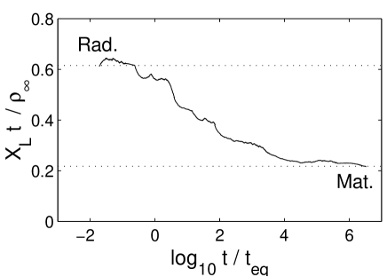
FIG. 1.: Evolution of $X_{L}(t)$. The dotted lines are the asymptotic values in the radiation and the matter eras.

We first perform string simulations with a string sampling spacing $1/1000$ of the simulation box sizes. The dynamic ranges cover from $0.05$ to $300$ $\eta_{\rm eq}$, where $\eta_{\rm eq}$ is the conformal time at radiation-matter energy density equality. We then perform the structure formation simulations with box sizes ranging from $20$–$120h^{-1}$Mpc, and a resolution of $128^{3}$–$512^{3}$. Figure 1 shows the evolution of $X_{L}$. We can see that the expected amount of energy was converted into loops in our simulations so that $X_{L}$ has the correct asymptotic behavior given by (3). However, the typical loop-size (and consequently their lifetime) does not approach scaling so rapidly and is therefore larger than physically expected for most of the duration in the simulations [4, 5]. To overcome this problem we rescale the loop lifetime according to equation (4). Thus the uncertainty in the average mass and therefore the lifetime of loops formed at a given time is quantified by the choice of the parameter $f$. The initial rms velocity of loops observed from the simulations is $\langle v^{2}_{*}\rangle^{1/2}\mathrel{\hbox to0.0pt{\lower 4.0pt\hbox{\hskip 1.0pt$\sim$}\hss}\raise 1.0pt\hbox{$>$}}0.7c$ throughout all the regimes.

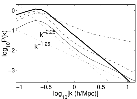
FIG. 2.: Small dynamic range power spectra of density perturbations seeded by long strings (thick solid), by loops with initial velocities $v_{*}$ switched to zero (dot-dashed), and by loops with $v_{*}$ determined by string network evolution (dashed and thin solid). The thin solid line includes the effect of gravitational decay of the loop energy, while the other two loop lines don’t but with loops removed after a period of time $\tau_{*}=t_{*}$.

Figure 2 shows the power spectrum of density perturbations induced by long strings and by cosmic string loops for $f=1$ for a small dynamic range from $2.5$ to $5\eta_{\rm eq}$. We can see that when compared with the spectrum induced by static loops (dot dashed), the amplitude of small-scale perturbations induced by moving loops (dashed) is clearly reduced by their motion. However, their large-scale power is higher because of the dependence of the gravitational interaction on the loop velocities, especially when they are relativistic. We also see that the gravitational decay of loop energy (thin solid) damps the overall amplitude of the power spectrum (dashed) by about a factor of 3. We notice that between the long-string correlation scale $k_{\xi}\approx 20/\eta\cite[cite]{[\@@bibref{Number}{AveShe2,AveShe4,AveShe3}{}{}]}$ and the scale $k_{\rm L}\approx 10k_{\xi}$, the slope of the loop spectrum (thin solid) is exactly the same as that of the long-string spectrum $n\approx-2.25$ [9]. We believe that this close correspondence is due to copious loop production being strongly correlated with long string intercommuting events and the collapse of highly curved long string regions [4], that is, near the strongest long string perturbations. Moreover, these correlations persist in time with the subsequent motion of loops and long strings lying preferentially in the same directions, a phenomenon which has been verified by observing animations of string network evolution. These correlations between loops and long strings, however, have a lower cutoff represented by the mean loop spacing $d_{\rm L}\sim k_{\rm L}^{-1}$. Below $d_{\rm L}$, the effects of individual filaments swept out by moving loops can be identified. In terms of the power spectrum, for $k<k_{\rm L}$ the loops are strongly correlated with the long strings and therefore reinforce the wake-like perturbations, while for $k>k_{\rm L}$ their filamentary perturbations increase the spectral index by about one to $n\approx-1.25$; this change is expected on geometrical grounds.

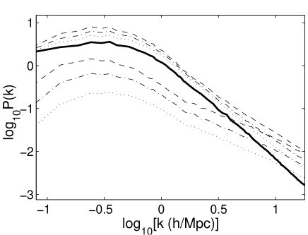
FIG. 3.: The lower set of 3 lines are ${\cal P}_{\rm L}(k)$ for $f=0.5$ (dotted), $1$ (dot-dashed) and $2$ (dashed). ${\cal P}_{\infty}(k)$ is plotted as a solid line. The upper set of lines are ${\cal P}_{\rm tot}(k)$ with corresponding line styles and $f$ values to the lower set of lines.

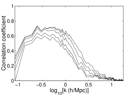
FIG. 4.: The correlation coefficient between the long-string and loop induced perturbations, with $f=0.5,1,2,4,6$ (downwards).

In figure 3 we plot the power spectra of density perturbations seeded by long strings ${\cal P}_{\infty}(k)$, by small loops ${\cal P}_{\rm L}(k)$, and by both loops and long strings ${\cal P}_{\rm tot}(k)$. The dynamic range here extends from $0.6$ to $7.5\eta_{\rm eq}$. As expected ${\cal P}_{\rm L}(k)$ scales more moderately than $f^{2}$ but more strongly than $f$ (see (11)). It is also apparent that the perturbations induced by long strings and by loops are positively correlated with ${\cal P}_{\rm tot}(k)>{\cal P}_{\rm L}(k)+{\cal P}_{\infty}(k)$ throughout the whole scale range. This positive correlation between loops and long strings boosts the large-scale ${\cal P}_{\infty}(k)$ by a factor of $1.5$, $1.8$ and $2.2$ to reach ${\cal P}_{\rm tot}(k)$ for $f=0.5,1$ and $2$ respectively, even if ${\cal P}_{\rm L}(k)$ is a relatively small fraction of ${\cal P}_{\infty}(k)$ on these scales.

Figure 4 shows the correlation coefficient between the long-string and loop induced perturbations. We see that long strings and loops are strongly positively correlated on large scales, but weakly correlated on small scales where the loops dominate the perturbations (also see figure 3). The threshold $k_{\rm t}$ between these two regimes must be significantly larger than $k_{\rm L}$ because, for $k<k_{\rm L}$, ${\cal P}_{\rm L}(k)$ is well below and roughly parallel to ${\cal P}_{\infty}(k)$ (see figures 2 and 3). We also verify that ${\cal P}_{\rm tot}(k)/{\cal P}_{\infty}(k)$ is approximately a constant for $k<k_{\rm L}\mathrel{\hbox to0.0pt{\lower 4.0pt\hbox{\hskip 1.0pt$\sim$}\hss}\raise 1.0pt\hbox{$<$}}k_{\rm t}$, which again provides strong evidence for the fact that loops behave as part of the long-string network on large scales.

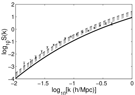
FIG. 5.: Comparison of the observational power spectrum [17] with ${\cal P}_{\infty}(k)$ (solid), and ${\cal P}_{\rm tot}(k)$ for $f=0.5,1,2,4,6$ (dashed, upwards), with a full dynamic range.

Given these properties of the string power spectra, one can easily construct a semi-analytic model for ${\cal P}_{\rm tot}(k)$ as for ${\cal P}_{\infty}(k)$ [7, 9]. We first multiply the structure function ${\cal F}(k,\eta)$ of ${\cal P}_{\infty}(k)$ by ${\cal J}(\eta,f)$ to account for the boost ${\cal P}_{\rm tot}(k)/{\cal P}_{\infty}(k)$ on large scales ($k<k_{\rm t}$), and then by a numerically verified form ${\cal H}(k,\eta,f)=[1+(k/k_{\rm t})^{4}]^{1/4}$ to account for the turnover for $k>k_{\rm t}(\eta,f)$. ${\cal J}(\eta,f)$ is calibrated phenomenologically from simulations deep in the radiation era through to those deep in the matter era. In the pseudo-scaling regime for the loop size, $k_{\rm t}$ is revealed to be at least $10k_{\xi}\approx 200/\eta$ depending on $f$. Thus we can carry out a full-dynamic-range integration to obtain ${\cal P}_{\rm tot}(k)$. In figure 5 we compare this ${\cal P}_{\rm tot}(k)$ and ${\cal P}_{\infty}(k)$ [7, 9] with observations [17]. The background cosmology is $\Omega_{\rm c}=0.15$, $\Omega_{\Lambda}=0.85$ and $h=0.7$, and we have used the COBE normalization $G\mu=1.7\times 10^{-6}$ [18] throughout. Since loops are point-like and they have little impact through the Kaiser-Stebbins effect on COBE-scale CMB anisotropies, we expect this normalization to be very weakly dependent on the value of $f$; indeed, loops were found to be negligible in ref. [19]. Thus we see from figure 5 that for $f\mathrel{\hbox to0.0pt{\lower 4.0pt\hbox{\hskip 1.0pt$\sim$}\hss}\raise 1.0pt\hbox{$>$}}0.5$, loops can contribute significantly to the total power spectrum and ease the large-scale bias problem seen previously [7, 9, 20]. Definite conclusions, therefore, about biasing in cosmic string models will need further advances in determining the magnitude of the parameter $f$, while all future large-scale structure simulations will now require the the inclusion of loops.

These additional complications in modelling cosmic string structure formation are most obvious on small scales, where even higher resolution and large dynamic range simulations will be required. However, we expect the power spectrum on large scales to be only weakly dependent on the details of loop formation. Within the present pseudo-scaling regime for loop size, we know that $k_{\rm t}\mathrel{\hbox to0.0pt{\lower 4.0pt\hbox{\hskip 1.0pt$\sim$}\hss}\raise 1.0pt\hbox{$>$}}k_{\rm L}\mathrel{\hbox to0.0pt{\lower 4.0pt\hbox{\hskip 1.0pt$\sim$}\hss}\raise 1.0pt\hbox{$>$}}10k_{\xi}$ as shown in figure 2 and discussed previously. Taking this extreme minimum $k_{\rm t}=10k_{\xi}$, then, we find that the semi-analytic model over the full dynamic range gives at most a $2\%$ difference in ${\cal P}_{\rm tot}(k)$ for $k<1h{\rm Mpc}^{-1}$ when the filament term ${\cal H}(k,\eta,f)$ is excluded from ${\cal F}(k,\eta)$ (for $\Omega_{\rm c}=0.15$, $\Omega_{\Lambda}=0.85$ and $h=0.7$). This means that although the simulations described in this letter are already on the verge of present computer capabilities, a further detailed study on small scales will improve only the overall normalization of ${\cal P}_{\rm tot}(k)$ but not the shape revealed here, which should be a robust feature. We note that advances in understanding loop formation mechanisms will also be crucial in quantifying the importance of the gravitational radiation background emitted by cosmic string network and its effect on large-scale structure and CMB anisotropies[21].

D Conclusion

In this Letter we have described the results of high-resolution numerical simulations of structure formation seeded by a cosmic string network with a large dynamic range, taking into account for the first time the loops produced by the network. We show that on large scales the loops behave like part of the long-string network and can therefore contribute significantly to the total power spectrum of density perturbations, provided their lifetime is not much smaller than one Hubble time. At present, the typical size and lifetime of loops formed by a string network remains to be studied in more detail; the problem is both computationally and analytically challenging. However, within the scale range of interest further developments in this area have the potential to affect the overall amplitude of the spectrum, while leaving the shape largely unchanged. The results presented here provide further encouragement for more detailed work on both the nature of cosmic string evolution and the large-scale structures they induce in cosmologies with $\Gamma\,=\,\Omega h\,=\,0.1$–$0.2$.

- [1] For a review see A. Vilenkin and E. P. S. Shellard, Cosmic strings and other topological defects (Cambridge University Press, 1994).
- [2] A. Vilenkin, Phys. Rev. Lett. 46, 1169 (1981)
- [3] J. Silk and A. Vilenkin, Phys. Rev. Lett. 53, 1700 (1984); Ya. B. Zel’dovich,Mon. Not. R. Astron. Soc.192, 663 (1980).
- [4] B. Allen and E. P. S. Shellard, Phys. Rev. Lett. 64, 119 (1990). E. P. S. Shellard and B. Allen, “On the Evolution of Cosmic Strings” in The Formation and Evolution of Cosmic Strings (Cambridge University Press: Cambridge) (1990).
- [5] D. P. Bennett and F. R. Bouchet, Phys. Rev. D 41, 2408 (1990).
- [6] A. Stebbins, “A New Picture for Cosmic String seeded structure formation” in The Formation and Evolution of Cosmic Strings (Cambridge University Press: Cambridge) (1990).
- [7] P. P. Avelino, E. P. S. Shellard, J. H. P. Wu, B. Allen, Phys. Rev. Lett. 81, 2008 (1998)
- [8] P. P. Avelino, E. P. S. Shellard, J. H. P. Wu, B. Allen, Astro-ph/9803120 (Ap. J. Lett. in press)
- [9] P. P. Avelino, E. P. S. Shellard, J. H. P. Wu, B. Allen, (in preparation).
- [10] P. P. Avelino, R. R. Caldwell, and C. J. A. P. Martins Phys. Rev. D 56, 4568 (1997).
- [11] R. A. Battye, J. Robinson and A. Albrecht, Phys. Rev. Lett. 80, 4847 (1998).
- [12] C. Contaldi, M. Hindmarsh & J. Magueijo, Astro-ph/9808201
- [13] P. P. Avelino, J. P. M. de Carvalho, Astro-ph/9810364
- [14] R. J. Scherrer, J. M. Quashnock, D. N. Spergel and W. H. Press Phys. Rev. D 39, 371 (1989).
- [15] B. Allen, E. P. S. Shellard Phys. Rev. D 45, 1898 (1992).
- [16] T. Vachaspati, A. Vilenkin Phys. Rev. D 31, 3052 (1985).
- [17] J. A. Peacock and S. J. Dodds, Mon. Not. R. Astron. Soc. 267, 1020 (1994).
- [18] B. Allen, R. R. Caldwell, S. Dodelson, L. Knox, E. P. S. Shellard, and A. Stebbins, Phys. Rev. Lett. 79, 2624 (1997).
- [19] B. Allen, R. R. Caldwell, E. P. S. Shellard, A. Stebbins and S. Veeraraghavan, Phys. Rev. Lett. 77, 3061 (1996)
- [20] A. Albrecht, R. A. Battye, and J. Robinson, Phys. Rev. Lett. 79, 4736 (1997).
- [21] P. P. Avelino, R. R. Caldwell Phys. Rev. D 53, 5339 (1996).