HYDRODYNAMIC SIMULATIONS OF COUNTERROTATING ACCRETION DISKS
Abstract
Time-dependent, axisymmetric hydrodynamic simulations have been used to study accretion disks consisting of counterrotating components with an intervening shear layer(s). Configurations of this type can arise from the accretion of newly supplied counterrotating matter onto an existing corotating disk. The grid-dependent numerical viscosity of our hydro code is used to simulate the influence of a turbulent viscosity of the disk. Firstly, we consider the case where the gas well above the disk midplane () rotates with angular rate and that well below () has the same properties but rotates with rate . We find that there is angular momentum annihilation in a narrow equatorial boundary layer in which matter accretes supersonically with a velocity which approaches the free-fall velocity. This is in accord with the analytic model of Lovelace and Chou (1996). The average accretion speed of the disk can be enormously larger than that for a conventional disk rotating in one direction. Under some conditions the interface between the corotating and counterrotating components shows significant warping. Secondly, we consider the case of a corotating accretion disk for and a counterrotating disk for . In this case we observed, that matter from the annihilation layer lost its stability and propagated inward pushing matter of inner regions of the disk to accrete. Thirdly, we investigated the case where counterrotating matter inflowing from large radial distances encounters an existing corotating disk. Friction between the inflowing matter and the existing disk is found to lead to fast boundary layer accretion along the disk surfaces and to enhanced accretion in the main disk.
These models are pertinent to the formation of counterrotating disks in galaxies and possibly in Active Galactic Nuclei and in X-ray pulsars in binary systems. For galaxies the high accretion speed allows counterrotating gas to be transported into the central regions of a galaxy in a time much less than the Hubble time.
Keldysh Institute of Applied Mathematics, Russian Academy of Sciences, Moscow, Russia
Department of Astronomy, Cornell University, Ithaca, NY 14853-6801
Space Research Institute, Russian Academy of Sciences,
Moscow, Russia; and
Department of Astronomy, Cornell
University, Ithaca, NY 14853-6801
and
Keldysh Institute of Applied Mathematics, Russian Academy of Sciences, Moscow, Russia
Accepted for publication in the Astrophysical Journal
Subject headings: accretion, accretion disks—galaxies: formation—galaxies: evolution—galaxies: nuclei—galaxies: spiral—galaxies
1 Introduction
The widely considered models of accretion disks have gas rotating in one direction with a turbulent viscosity acting to transport angular momentum outward (Shakura 1973; Shakura & Sunyaev 1973). However, recent observations indicate that there may be more complicated disk structures in some cases on a galactic scale, in galactic nuclei, and in disks around compact stellar mass objects. Studies of normal galaxies have revealed counterrotating gas and/or stars in many galaxies of all morphological types - ellipticals, spirals, and irregulars (Rubin 1994a, 1994b; Galletta 1995). In elliptical galaxies, the counterrotating component is usually in the nuclear core and may result from merging of galaxies with opposite angular momentum.

In a number of spirals and S0 galaxies, counterrotating disks of stars and/or gas have been found to co-exist with the primary disk out to large distances ( kpc), with the first example, NGC 4550, discovered by Rubin, Graham, & Kenney (1992). Of interest here is the “Evil Eye” galaxy NGC 4826 in which the direction of rotation of the gas reverses going from the inner ( km/s) to the outer disk ( km/s) with an inward radial accretion speed of more than km/s in the transition zone, while the stars at all radii rotate in the same direction as the gas in the inner disk which has a radius pc (Braun et al. 1994; Rubin 1994a, 1994b). The large scale counterrotating disks probably do not result from mergers of flat galaxies with opposite spins because of the large vertical thickening observed in simulation studies of such mergers (Hernquist & Barnes 1991; Barnes 1992). Thakar & Ryden (1996) discuss different possibilities, (a) that the counterrotating matter comes from the merger of an oppositely rotating gas rich dwarf galaxy with an existing spiral, and (b) that the accretion of gas occurs over the lifetime of the galaxy with the more recently accreted gas counterrotating. Subsequent star formation in the counterrotating gas may then lead to counterrotating stars. Counterrotating gas may have a strong interaction with the gas resulting from mass loss by corotating stars (Braun et al. 1994). Further, the two-stream instability between counterrotating gas and corotating stars can be important for gas accretion (Lovelace, Jore, & Haynes 1996).
Accretion of counterrotating matter onto an existing corotating disk around a massive black hole may occur in an Active Galactic Nucleus (AGN). The counterrotating matter may come from recently captured material from a galaxy merger, from a tidally disrupted molecular cloud, or from a star. Tidal disruption of a star by the central black hole may release essential part of the star in the form of gas (Rees 1990; Shlosman, Begelman, & Frank 1990; Khokhlov & Melia 1996). There is a significant probability that this gas has angular momentum opposite to that of the main disk. This can lead to formation of small disks with opposite angular momentum in the center of a galaxy (Melia 1994). This was studied using 3D numerical simulations by Ruffert (1994), Ruffert & Melia (1994). The retrograde disks may also slow down the rotation of the central black hole (Moderski & Sikora 1996). The greatly enhanced accretion rate for counterrotating matter in the presence of a corotating disk may give outbursts of AGN.
Another situation where counterrotating matter may encounter an existing corotating disk is in low mass X-ray binary sources where the accreting, magnetized rotating neutron stars are observed to jump between states where they spin-up and those where they spin-down. Nelson et al. (1997a, b) and Chakrabarty et al. (1997) have proposed that the change from spin-up to spin-down results from a reversal of the angular momentum of the wind supplied accreting matter. Their suggestion is based on the recent BATSE observations which show a rapid change from spin-up to spin-down evolution of some X-ray pulsars. This is difficult to explain with conventional theory (see, however, Lovelace, Romanova, & Bisnovatyi-Kogan 1998). Reversal of the angular momentum of accreted matter in wind-fed binaries was observed in the two-dimensional simulations by Blondin et al. (1990), Livio et al. (1991), and Bisikalo et al. (1996).
An important open problem is to understand the interaction of counterrotating gaseous disks. Earlier two-dimensional simulations used either collisionless particles to represent a system of stars (Davies & Hunter 1997) or “sticky” particles (Thakar & Ryden 1996, and references therein) to represent a system of clouds. The sticky particle interaction gives only a rough representation of a viscous fluid. When both components of a counterrotating system are gaseous, it is important to understand their interaction using the full equations of hydrodynamics including the viscous transport of angular momentum. Hydrodynamic interaction of a galactic disk with infalling matter of a non-rotating corona was investigated by Falcke & Melia (1997) using a one dimensional approach. They showed that this interaction may lead to significant evolution of the disk.
Lovelace & Chou (1996) (hereafter LC) developed an analytic theory of the viscous hydrodynamic interaction of counterrotating gaseous disks basing on the viscosity model of Shakura (1973) and Shakura & Sunyaev (1973).
Here, we present the results of two-dimensional, time-dependent hydrodynamic simulations of counterrotating accretion disks. We investigate three main models which are sketched in Figure 1.
Model I is shown in the top sketch of Figure 1: In this case the accretion disk consists of counterrotating gaseous components with gas above the disk midplane rotating with angular rate , and that below rotating at rate . The interface between the components at constitutes a supersonic shear layer. A configuration of this type may arise from the accretion of newly supplied counterrotating gas onto an existing corotating disk. For this case the analytical model of Lovelace & Chou (1996) proposed that matter approaching the equatorial plane from above and below has angular momenta of opposite signs with the result that there is angular momentum annihilation at . This matter loses its centrifugal support and accretes at essentially free-fall speed.
Model II is shown in the middle sketch in Figure 1: In this model we consider that where there is a corotating () accretion disk (the “old” disk) for and a counterrotating () disk (the “new” disk) in the region . This case is clearly pertinent to the “Evil Eye” galaxy NGC 4826.
Model III is shown in the lower sketch of Figure 1: This model corresponds to inflow of counterrotating matter which interacts with an existing corotating disk. In this case annihilation of angular momentum occurs on the surface of the existing disk and this can lead to fast accretion.
In §2 we discuss the pertinent fluid dynamical equations for axisymmetric accretion, the initial and boundary conditions, and the numerical method used. In §3 - §5 we discuss results obtained for Models I-III. We present astrophysical examples in §6. In §7 we give conclusions of this work.


2 Mathematical Model
2.1 Basic Equations
The axisymmetric flows are described by the inviscid hydrodynamic equations (Euler equations) in spherical, inertial coordinates (with the equatorial plane):
| (1a) |
| (1b) |
| (1c) |
| (1d) |
| (1e) |
Here, is the density; the flow velocity, with components ; the pressure; the gravitational potential; the full specific energy ; the specific internal energy; and the full specific enthalpy, . An equation of state is necessary, and we assume the ideal gas equation,
where is the usual ratio of heat capacities. The gravitational potential is considered to be the Newtonian potential of the central object.
That is, we assume that the self gravity of the disk is negligible.
2.2 Alternative Form of Energy Equation
In our early disk simulations we found that the energy equation taken in divergent form (1e) can lead to inaccurate results. The reason for this is the large value of the azimuthal velocity and the corresponding kinetic energy in comparison with other velocities/energies. The relatively small quantity is determined from (1e) inaccurately in this case.
To correct this problem we now have excluded the -velocity part of the energy from the energy equation by writing
and subtracting this equation from equation (1e) to obtain another divergent form of energy equation,
| (2) |
where and are the ‘reduced’ (poloidal) full specific energy and the ‘reduced’ (poloidal) full specific enthalpy, and , respectively. In all of our calculations equation (2) was used instead (1e).
2.3 Characteristic Scales
The physical quantities have evident characteristic scales: Distances are measured in terms of the inner radius of the disk . Velocities are measured in terms of the Keplerian velocity at the inner edge of the disk, . Time is measured in units of the period of revolution of the inner edge of the disk . The density is given in relative units.

2.4 Initial Equilibria
We have adopted spherical coordinates for our simulations in order to obtain a good match of the grid to the accretion disk which in general has a thickness in the direction () increasing with . However, for convenience our figures and initial disk equilibria described in this subsection are given in coordinates.
2.4.1 Initial Conditions 1
A disk equilibrium with , , but is described by the equations
where the position and velocity are now dimensionless as mentioned.
With the assumption of a polytropic gas , where is the polytropic index, , the common solution of equations (3) can be written as
where is the specific enthalpy, , with a constant, the sound speed, and an arbitrary function depending only on . The angular velocity is given in this case as
The disk boundary is determined by the condition or . If we assume the Keplerian law for angular velocity, , then
and
where and are the values at the point . The disk boundary in this case is
so the disk thickness diverges at some very large radius outside the region of interest. A sample density distribution is shown in Figure 2. Hereafter, we refer to this case as Initial Condition 1. This was used for the runs described in §3 and §4.


2.4.2 Initial Conditions 2
A second equilibrium disk model was used in our simulations. For this we took the disk boundary () to have the form
where and are parameter determining disk radial size and thickness. The rotation (slightly sub-Keplerian), enthalpy, and density for this case are:
The density distribution for this case is shown in Figure 3. Hereafter, we refer to this case as Initial Conditions 2.
For building equilibria we have used both a rotation law based approach and one based on the shape of the disk surface. For the first case, the equilibria are found for known rotation law according to the chain . For the second case, a known disk surface is used according to the chain . Abakumov et al. (1996) use an analogous approach.
2.5 Boundary Conditions
Simulations were performed in the region , .
The outer boundary conditions are treated following the method used by Sawada based on solving of the Riemann problem (see, e.g., Sawada, Matsuda, & Hachisu 1986; Sawada & Matsuda 1992). These boundary conditions were used for Models I and II. However, for Model III different boundary conditions are applied in that matter is considered to inflow supersonically through part of the outer boundary.
We assume that all matter coming into the sphere is absorbed. On the axis, , we of course have and .
No symmetry is assumed with respect to the equatorial plane.
2.6 Numerical Method and Viscosity Treatment
An explicit Lax-Friedrichs finite-difference scheme with flux correction in Chakravarthy-Osher (Chakravarthy & Osher 1985) form was used. This scheme is order of approximation in time and order of approximation in space and is oscillation-free near discontinuities. The combined Lax-Friedrichs-Osher scheme was suggested in work by Vyaznikov, Tishkin, & Favorsky (1989).
Figure 4 shows the non-homogeneous grid used in the simulations. The radial grid increment increases outwards exponentially, , where . The grid increases in a similar way going away from the equatorial plane. For a disk which has thickness increasing with , this type of grid gives a more uniform distribution of cells within the disk including its central regions. In the simulations we used grids of of or in some cases.
The simulation method used naturally has numerical viscosity. With a fixed grid, we cannot vary the numerical viscosity, but we can investigate its influence. The coefficient of numerical viscosity can be represented as , where is the sound speed, is the size of the grid. This expression for is analogous to that proposed by Shakura (1973) and Shakura & Sunyaev (1973) for the turbulent viscosity of accretion disks, , where is the thickness of the disk, and is a dimensionless parameter. We calculated the steady accretion for a disk rotating in one direction and observed the accretion due to the numerical viscosity. Using the formula for the accretion speed of a viscous accretion disk, , we estimated that for for a grid and for for a grid, and decreases to at the outer radii. A challenge for future work is the inclusion of a true viscosity.
We investigated three different models of counterrotating accretion flows which correspond to different possible astrophysical situations. The first model corresponds to disks counterrotating in the direction (Model I, §3). The second corresponds to disks counterrotating in the direction (Model II, §4). The third corresponds to counterrotating gas infalling onto a pre-existing corotating disk (Model III, §5).


3 Disk Counterrotating in the direction: Model I
Here, we discuss simulation results for Model I where initially the upper half of the disk () is corotating () while the lower half () is counterrotating (). This case was treated analytically by LC, and therefore we have a test both of the LC theory and of our simulation code.
First in §3.1, we check the initial equilibrium disk for the conventional case of unidirectional disk rotation. Secondly in §3.2, we investigate the counterrotating disk for , which is close to isothermal. This value of close to unity mimics conditions of strong radiative cooling. In this subsection we compare the simulations results with the predictions of LC where radiative cooling is included. In these subsection we used a grid. Thirdly in §3.3, we discuss the cases and which corresponds to non-isothermal conditions where numerical viscous heating is significant. In this subsection we used a grid.


3.1 Conventional Accretion Disk
As a calibration of our simulation code, we investigated a conventional accretion disk which rotates in only one direction. The disk evolves as a result of the relatively small numerical viscosity of the code. We took Initial Conditions 1 (see §2.4.1) with and performed long-term numerical simulations of this disk. We observed that the disk shape did not change during many periods of rotation of the inner radius of the disk. Figure 5 shows the iso-density contours distribution at . The evolved disk is close to that at (see Figure 2), excluding the inner part, where the thickness of the disk is very small (comparable with the grid size), and the numerical viscosity has a noticeable influence.
3.2
This case is close to isothermal and is closest to the LC analytical model where both viscous heating and radiative cooling are included.
We took Initial Conditions 1 for the initial conditions for the density and velocity of the disk (see Figure 2), but put the angular velocity in the lower-half of the disk () opposite to the angular velocity of the upper-half (). Figure 6 shows that matter starts to rapidly flow radially inward in a narrow region near the midplane of the disk. The poloidal flow near the midplane is supersonic, and the radial inflow velocity increases as decreases.
Figure 7 shows the radial variation of the radial velocity in the midplane of the disk at different times. The velocity distribution changes only gradually with time. The velocity close to the gravitating center, is much larger than velocity in the outer regions of the disk, . Note, that for , the radial inflow velocity is close to the free-fall velocity . An inflow velocity is predicted by LC. Velocity is strongly supersonic with Mach number . Figure 7 shows that velocity distribution along the disk is almost the same during the long time. Figure 8 shows the dependence of density on radial distance.
The density of the disk decreases with time, specifically in the inner regions of the disk. Both, the velocity and density show small-scale wave-like variations as a function of radius.
Figure 9 shows the observed vertical () variation of the radial and azimuthal velocities in the disk at and the theoretical dependencies calculated by LC. The dimensionless vertical length was introduced by LC as , where is the characteristic half-thickness of the boundary layer in which most of the radial inflow of matter occurs. Consistent with LC, we find that over most of the disk surface, where is the full disk half-thickness. At , we find . One can see that radial inflow velocity has a maximum in the midplane of the disk and decreases to small values at large . Note that we observe weak outflows for where . Similar outflows were predicted by LC (the solid curves). The azimuthal velocity grows with increasing and reaches the Keplerian velocity for . There is also a region, where the azimuthal velocity is slightly larger than Keplerian velocity, . A similar region was predicted by LC (see solid curve in Figure 9).
The conditions considered by LC were different from the initial conditions considered for our simulations. Thus, it appears that the main features of vertically stratified counterrotating flows do not depend strongly on the initial conditions. At longer times in our simulation runs, the region of fast equatorial flow becomes somewhat thicker. Overall the simulation results are close to the predictions of the analytic model of LC. Although the analytic model includes viscous heating and radiative cooling, these almost compensate each other with the result the model is close to the simulations which has almost isothermal conditions and no radiative cooling.
Figure 10 shows the radial dependence of the mass accretion rate at different times, and that for a disk rotating in one direction at time (§3.1). The mass accretion rate for the counterrotating disk can be written as
where the numerical coefficient (3.25) is obtained from Figure 9. In that the surface mass density of the disk is , the average accretion speed is . For comparison the mass accretion rate for a conventional disk rotating in one direction (Shakura 1973; Shakura & Sunyaev 1973) is
In this case the average accretion speed is . For a conventional accretion disk, the quantity is commonly thought to be much smaller than unity. For example, for , , and , .
3.3 and
We also did simulations of vertically stratified counterrotating disks for and which correspond to non-isothermal conditions were the affect of viscous heating is more important. We find in general that after a given time and for a given numerical grid, the temperatures in the disk increase as increases. Thus, the disk thickness is larger for larger . On the other hand for fixed , the temperature in the disk decreases gradually as the resolution increases. Here, we performed simulations with the grid . To increase the resolution even more (to decrease viscosity) we performed simulations of only part of the disk: .
At early times (), the flow in the equatorial plane of the disk was similar to that for . However, for longer times the region of fast poloidal inflow begins to warp. Figure 11 shows contours of density and velocity vectors of the disk at two times. The amplitude of the warp of the interface between corotating and counterrotating flows grows. After a fixed time the warp amplitude is a strongly increasing function of . For the fractional warp amplitude is very small for all times. However, the warp amplitude for is , and for it is both at with the same resolution as used in Figure 11. The warp amplitude is of the order of the disk half-thickness . For the dominant radial wavelength is while for there is a wide spectrum of wavelengths from to . The warping is suppressed by low grid resolution.
The warping may represent a Kelvin-Helmholtz type of instability driven by the shear in the poloidal flow. The tidal gravitational force of the central object, , acts to keep the warp amplitude from growing without bound. Note that Kelvin-Helmholtz instabilities driven by the shear in the azimuthal flow are suppressed in our simulations which are axisymmetric. Alternatively, the disk warping may be due to unsymmetrical (top/bottom) heating of the disk which gives an excess pressure in say the bottom half of the disk which displaces the disk upward. Plots of the pressure, density, and temperature through the disk as shown in Figure 12 support this simple explanation.

4 Disk Counterrotating in the Direction: Model II
Here, we treat Model II which is shown schematically in the middle panel of Figure 1. In this model the inner part of the Keplerian disk () rotates in the positive direction whereas the outer part () rotates in the opposite direction. The transition between positive and negative azimuthal velocity was centered at and extended over the narrow region . This transition region is small, involving only grid points in the radial direction for a mesh size of . The boundary condition at the right side of the disk was taken the same as in Model I. Simulations were performed for and . Results are presented for .
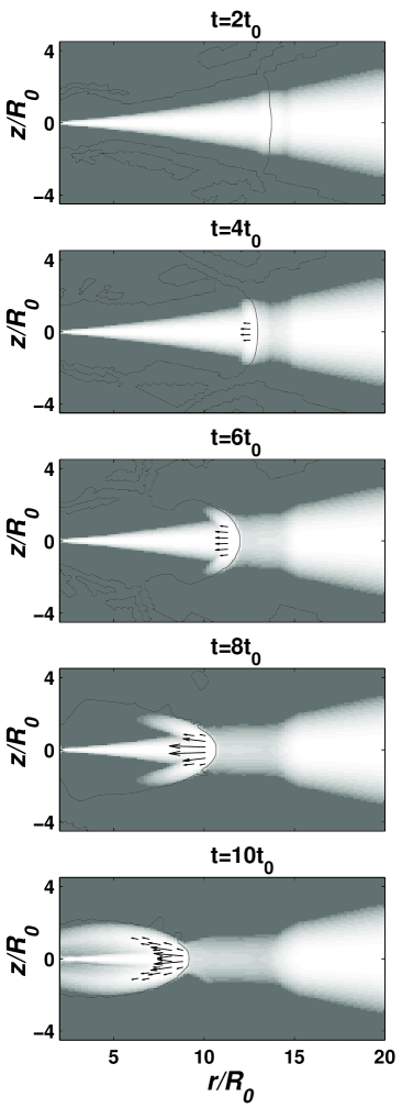
In our simulations, matter in the transition zone with low angular momentum flows rapidly inward compressing matter at smaller radii as shown in Figures 13 and 14. This inflow sets up a density wave which propagates inward in the disk. The matter behind the wave has lower density. The speed of propagation of the wave grows with time and reaches a maximum value equal to about one half of the free-fall velocity (see Figure 14). The azimuthal velocity in the wave is sub-Keplerian with in inner part of the disk. Matter behind the wave (at larger ) has opposite velocity, with a magnitude somewhat smaller than the local Keplerian velocity (see Figure 14). The wave propagates supersonically, with Mach number . The Mach number grows as the wave moves inward (see Figure 14).
The shock wave propagating initially at times is not a standard shock wave, because it has significant angular momentum, and its formation and propagation is based on the deficit of angular momentum of the matter of the wave and an inbalance of gravitational and centrifugal forces. The density and velocity jumps are much larger than in the case of standard shock wave (see Figure 14). This wave resembles a soliton-type wave. A similar type of wave was observed in accretion disks where a local deficit of angular momentum was caused by magnetically driven outflows (Lovelace, Romanova, & Newman 1994; Lovelace, Newman, & Romanova 1997). Note that the solid line in Figure 13 indicates the boundary between corotating and counterrotating components. The density wave reaches during (ten periods of rotation of the inner edge of the disk). For longer times, matter started to “reflect” from the inner regions and move outward.
The effective collapse of the inner disk can be understood by considering the details of the model used. The density of the disk is constant along the equatorial plane so that the mass of the equidistant rings increases outwards, , so that the mass of ring at is times larger than a ring at . At the same time the angular momentum of the rings increases outwards as , so that the angular momentum of inner ring is times smaller than of the ring at . The layer between counterrotating disks has pretty large mass and zero angular momentum. It is not centrifugally supported and falls down to the center. It accumulates the matter of the inner regions of the disk and their angular momentum. But absorbed angular momentum is not sufficient to rich the centrifugal barrier.
The thickness of the boundary layer in which there is annihilation of angular momentum depends on the viscosity. For a larger viscosity, the layer is thicker and the propagating wave is stronger. The fast inward propagation of such a wave in a disk around a black hole would give an outburst in the luminosity as the wave reaches the black hole. This represents a possible mechanism of generating outbursts in Active Galactic Nuclei, for example.
5 Inflow of Counterrotating Gas onto a Corotating Disk: Model III
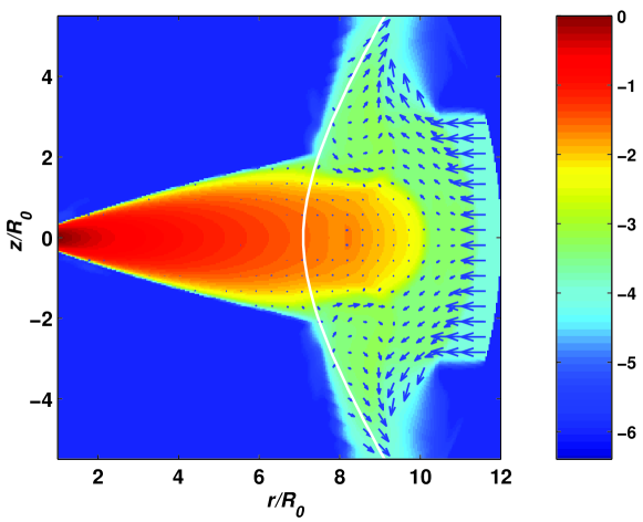
Here, we discuss Model III which is shown schematically in the bottom panel of Figure 1. In this case counterrotating gas of relatively low density inflows with significant poloidal speed and encounters an existing Keplerian disk. For the simulations, we took Initial Conditions 2 (§2.4.2) corresponding to a finite radius, slightly sub-Keplerian, corotating disk (see Figure 3). The effective outer radius of this disk was taken to be at . At the outer, right-hand boundary of the computational region, matter is launched into the simulation region from the part of the boundary with radial velocity and azimuthal velocity . When both: the “target” disk and incoming matter rotate in the same direction, then incoming matter moves inward only until it reaches the centrifugal barrier (see white line on Figure 15), then it stops, and moves in the directions away from the disk surface.

Figure 15 shows the observed behavior of density and velocity in this case. Note, that in this case we observe only very small accretion connected with finite viscosity of the disk. This case was considered for reference.
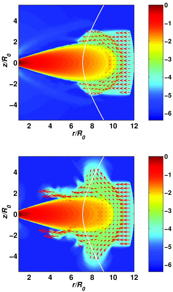
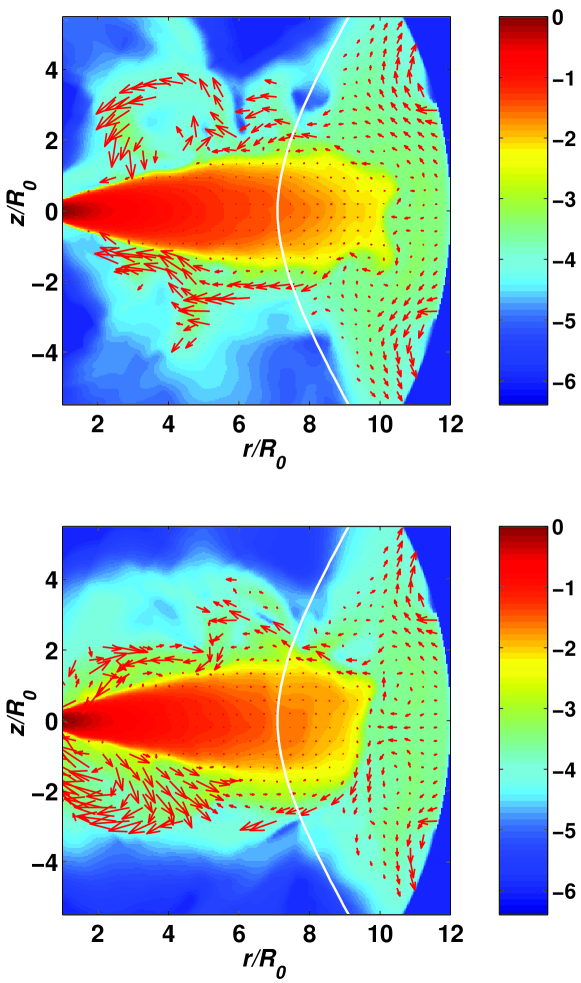
When the inflowing matter rotates in the opposite direction to that of the “target” disk, then it also reaches a centrifugal barrier. However, a non-negligible fraction of the inflowing matter interacts with the disk causing angular momentum annihilation. For this case the fraction is . Figures 16 and 17 show the evolution. One can see from Figure 16 (top and bottom panels), that at times , the gas starts to flow along the surfaces of the target disk. Later, at , it flows strongly along the surfaces (see top panel of Figure 17). The radial velocity of matter flowing along the surfaces is . Later, the layer became thicker owing to viscous dissipation and the flow became more chaotic (Figure 17, bottom panel). The temperatures increased few times in the surface layer. Here, we should remind, that viscous heating is included, but cooling is not. If radiative cooling balances viscous heating, then this surface layer may survive much longer than in the simulation. The surface flow is similar in some respects to that observed in Model I (§3). As in Model I, we also observed the increase of the radial inflow velocity with decreasing .
In this model, we also observed an interaction similar to that investigated in Model II. Namely, the interaction occurred not only along the surfaces of the disk but also through the cross section of the disk. As a result, accretion was enhanced inside the main disk as in Model II. Compared with Model II, the density of counterrotating matter is much smaller than that of the “target” disk. For this reason the interaction did not lead to dramatic wave formation. The radial velocity of viscous flow inside the disk increased by a factor of , and matter flux increased by a similar factor. However, the velocity of accretion of the main disk remained much smaller than the free-fall velocity.
Note, that during this violent evolution of the outer layers of the disk, the main part of the “target” disk was very stable, the density did not change appreciably, and the radial velocities remained small.
Figure 18 shows the time evolution of the matter flux through the cylindrical surface . It increases by a factor compared with the initial flux. For it increases mainly as a result of surface layer accretion. Later, there is also enhanced accretion from the main part of the “target” disk. A fraction about of the incoming matter is accreted.
6 Two Applications
Here, we briefly consider two applications of our results to accretion disks. One is related to galaxies and the second to X-ray pulsars.
6.1 Galaxies
In some disk galaxies, counterrotating gas and/or stars are observed (e.g., Rubin 1994a, 1994b; and Galletta 1995). Even though the present work treats Keplerian disks, we can nevertheless make estimates based on our hydrodynamic results. The rotation curves of galactic disks are flat (const) over a significant range of distances owing in part to a spheroidal distribution () of dark matter. Although this rotation curve is quite different from Keplerian, the analytic viscous accretion flows are nearly the same for flat and Keplerian rotation curves (LC). The reason is that the boundary layer formed between the oppositely rotating components, where angular momentum is annihilated and fast accretion occurs, does not depend strongly on the radial dependence of .
We consider the situation where a counterrotating cloud of hydrogen of mass is captured into an equatorial orbit of radius kpc. Model III is pertinent to this situation. Interaction between the counterrotating cloud and existing corotating gas (assumed mass ) in the galaxy leads to fast boundary layer accretion along the top and bottom surfaces of the galactic disk with average accretion speed , where we have adapted the results of §3 to Model III which has two boundary layers, and where we have used the circular velocity of the galaxy const rather than the Keplerian velocity . The time-scale for this fast accretion to the center of the galaxy is therefore
where we have assumed . For the reference values of equation (9a) and assuming that the cloud mass is accreted in a time , the mass accretion rate is
where the factor of two accounts for the fact that half of the accreted gas is from the existing disk. Note that the accretion time-scale is much less than the Hubble time.
6.2 X-Ray Pulsars
Nelson et al. (1997a,b) and Chakrabarty et al. (1997) have proposed that the change from spin-up to spin-down of X-ray pulsars in binary systems results from a reversal of the angular momentum of the wind supplied accreting matter. The matter inflowing to the pulsar is assumed to be supplied at a constant rate at a radius in the equatorial plane of the binary system. Initially, the pulsar is assumed to have a conventional, corotating disk. Then, due to some disturbance, the sense of rotation of the supplied matter reverses so that it is counterrotating. Model III is again pertinent to this situation. The ‘new’ counterrotating matter encounters the ‘old’ corotating disk. Interaction between the ‘new’ and ‘old’ matter leads to fast boundary layer accretion with average accretion speed . The time-scale for this fast accretion to reach the pulsar is
where we have again assumed . The sign of the angular momentum carried by the boundary layer flows at the much smaller Alfvén radius , which determines the spin-up or spin-down of the pulsar, is uncertain from the present work. If this has the sense of the counterrotating material supplied at , then a rapid switch between spin-up and spin-down of the pulsar would occur with time scale of order .
On a much longer time-scale, inflowing counterrotating matter will ‘use up’ the old corotating disk. This time scale is simply the accretion time for a disk rotating in one direction,
A further time interval is required for establishment of an equilibrium disk rotating in the opposite direction to the original disk.
7 Conclusions
Time-dependent, axisymmetric hydrodynamic simulations have been used to study Keplerian accretion disks consisting of counterrotating components. The simulation code used for the study has a numerical viscosity which is calibrated by study of the accretion of a disk rotating in one direction. Different grid resolutions were used to study the influence of the numerical viscosity. Our simulation model does not include radiative cooling. Therefore, different values of the specific heat ratio from to were used in order to assess the influence of heating due to the numerical viscosity. A small value of corresponds to almost isothermal conditions.
Different cases were considered. In Model I, the gas well above the disk midplane rotates in one direction and that well below has the same properties but rotates in the opposite direction. In this case there is angular momentum annihilation in a narrow equatorial boundary layer in which matter accretes supersonically with a velocity which approaches the free-fall velocity. The average accretion speed of the disk can be enormously larger than that for a conventional viscosity disk rotating in one direction. For a much lower viscosity (when we took a small part of the region and calculated it with a grid resolution of ), the interface between the corotating and counterrotating components shows significant warping, which is probably a type of Kelvin-Helmholtz instability. We observed that a large viscosity suppresses this instability.
In Model II, we considered the case where the inner part of the disk corotates while the outer part counterrotates. In this case a new equilibrium inner disk forms with a low density gap between inner and outer disks. In Model III we investigated the case where low-density counterrotating matter inflowing from large radial distances encounters an existing corotating disk. Friction between the inflowing matter and the existing disk is found to lead to fast boundary layer accretion along the disk surfaces, while interaction of the disk with counterrotating matter at large radii, leads to enhanced accretion in the main body of the disk. We observed that the boundary layer accretion is a temporary phenomenon, because the interaction of the dense disk and low-density counterrotating gas leads to heating of this gas. However, the interaction at large radii is more steady and leads to continuous enhanced accretion in the main disk.
These models are pertinent to the formation of counterrotating disks in galaxies, in Active Galactic Nuclei, and in X-ray pulsars in binary systems. For galaxies the high accretion speed allows counterrotating gas to be transported into the central regions of a galaxy in a time much less than the Hubble time.
It is clear that inclusion of the important role of Kelvin-Helmholtz (KH) instabilities in counterrotating disks requires D simulations and this will be the subject of a future paper. For example, note that in Model I if the flow is treated as a vortex sheet without radial inflow, then a local stability analysis with the wavevector) indicates unstable KH warping for wavenumbers and a maximum growth rate of (LC; Choudhury & Lovelace 1986). To account for this non-axisymmetric warping instability of the disk, we clearly need simulations. In Model II, a local stability analysis of the interface between the inner and outer disks indicates unstable KH warping for and a maximum growth rate of . Also in this case 3D simulations are needed.
A number of further developments are planned. Simulations explicitly including an viscosity are desirable for detailed comparison with theory. Explicit inclusion of radiative cooling is equally important. Also, 3D simulations are needed to investigate the Kelvin-Helmholtz instability.
One of the authors (MMR) thanks Prof. R. Giovannelli and D. Dale for helpful discussions. We thank an anonymous referee for many constructive comments on an earlier version of this work. This work was supported in part by NSF grant AST-9320068. OAK and VMC were supported in part by the Russian Federal Program “Astronomy” (subdivision “Numerical Astrophisics”) and by INTAS grant 93-93-EXT. Also, this work was made possible in part by Grant No. RP1-173 of the U.S. Civilian R&D Foundation for the Independent States of the Former Soviet Union. The work of RVEL was also supported in part by NASA grant NAG5 6311.
REFERENCES
Abakumov, M.V., Mukhin, S.I., Popov, Yu.P., & Chechetkin, V.M. 1996, Astron. Reports, 40, 366
Barnes, J.E. 1992, ApJ, 393, 484
Bisikalo, D.V., Boyarchuk, A.A., Kuznetsov, O.A., & Chechetkin, V.M. 1996, Astron. Reports, 40, 662
Blondin, J.M., Kallman, T.R., Fryxell, B.A., & Taam, R.E. 1990, ApJ, 356, 591
Braun, R., Walterbos, R.A.M., Kennicutt, R.C.,Jr., & Tacconi, L.J. 1994, ApJ, 420, 558
Chakrabarty, D., et al. 1997, ApJ, 481, L101
Chakravarthy, S., & Osher, S. 1985, AIAA Paper No. 85-0363
Choudhury, S.R., & Lovelace, R.V.E. 1986, ApJ, 302, 188
Davies, C.L., & Hunter, J.H.,Jr. 1997, ApJ, 484, 79
Falcke, H., & Melia, F. 1997, ApJ, 479, 740
Galletta, G. 1995, in Barred Galaxies, ASP Conf. Ser., V. 91, ed. R.Buta, D.Crocker, & B.Elmegreen (San Francisco: ASP), 429
Hernquist, L.E., & Barnes, J.E. 1991, Nature, 354, 210
Khokhlov, A., & Melia, F. 1996, ApJ, 457, L61
Livio, M., Soker, N., Matsuda, T., & Anzer, U. 1991, MNRAS, 253, 633
Lovelace, R.V.E., & Chou, T. 1996, ApJ, 468, L25 (LC)
Lovelace, R.V.E., Jore, K.P., & Haynes, M. P. 1997, ApJ, 475, 83
Lovelace, R.V.E., Romanova, M.M., & Newman, W.I. 1994, ApJ, 437, 136
Lovelace, R.V.E., Newman, W.I., & Romanova, M.M. 1997, ApJ, 484, 628
Lovelace, R.V.E., Romanova, M.M., & Bisnovatyi-Kogan, G.S. 1998, ApJ Lett., submitted
Melia, F. 1994, ApJ, 426, 577
Moderski, R., & Sikora, M. 1996, A&AS, 120C, 591
Nelson, R.W., et al., 1997a, in ASP Conf. Proc., Accretion Phenomena and Related Outflows, ed. G.Bicknell, L.Ferrario, & D.Wickramasinghe (San Francisco: ASP), p. 256
Nelson, R.W., et al., 1997b, ApJ, 488, L117
Rees, M.J. 1990, Science, 247, 817
Shlosman, I., Begelman, M.C., & Frank, J. 1990, Nature, 345, 679
Rubin, V.C. 1994a, AJ, 107, 173
———. 1994b, AJ, 108, 456
Rubin, V.C., Graham, J.A., & Kenney, J.D.P. 1992, ApJ, 394, L9
Ruffert, M. 1994, ApJ, 427, 342
Ruffert, M., & Melia, F. 1994, A&A, 288, L29
Sawada, K., Matsuda, T., & Hachisu, I. 1986, MNRAS, 219, 75
Sawada, K., & Matsuda, T. 1992, MNRAS, 255, 17P
Shakura, N.I. 1973, SvA, 16, 756
Shakura, N.I., & Sunyaev, R.A. 1973, A&A, 24, 337
Thakar, A.R., & Ryden, B.S. 1996, ApJ, 461, 55
Vyaznikov, K.V., Tishkin, V.V., & Favorsky, A.P. 1989, Mathematical Modelling, 1, 79 (in Russian)