3D numerical cosmological radiative transfer in an inhomogeneous medium

Abstract

A numerical scheme is proposed for the solution of the three-dimensional radiative transfer equation with variable optical depth. We show that time-dependent ray tracing is an attractive choice for simulations of astrophysical ionization fronts, particularly when one is interested in covering a wide range of optical depths within a 3D clumpy medium. Our approach combines the explicit advection of radiation variables with the implicit solution of local rate equations given the radiation field at each point. Our scheme is well suited to the solution of problems for which line transfer is not important, and could, in principle, be extended to those situations also. This scheme allows us to calculate the propagation of supersonic ionization fronts into an inhomogeneous medium. The approach can be easily implemented on a single workstation and also should be fully parallelizable.

1 Introduction

Understanding the effect of the radiation field on the thermal state of interstellar and intergalactic gas is important for many areas of astrophysics, and in particular for star and galaxy formation. Of special interest for cosmological structure formation are the epoch of reionization of the Universe (Gnedin & Ostriker 1997, Miralda-Escudé et al. 1998), the effects of self-shielding on the formation of disk and dwarf galaxies (Navarro & Steinmetz 1997, Kepner et al. 1997) and the absorption properties of Ly$\,\alpha$ clouds (Katz et al. 1996, Meiksin 1994). While our knowledge of the physics of large-scale structure and galaxy formation has benefited significantly from numerical N-body and gas-dynamical models (see, e.g., Zhang et al. 1998, and references therein), there is very little that has been done to include radiative transfer (RT) into these simulations. Challenges seem to abound, not least of all, the fact that the intensity of radiation in general is a function of seven independent variables (three spatial coordinates, two angles, frequency and time). While for many applications it has been possible to reduce the dimensionality (e.g. to build realistic stellar atmosphere models), the clumpy state of the interstellar or intergalactic medium does not provide any spatial symmetries. Moreover, coupled equations of radiation hydrodynamics (RHD) have very complicated structure, and are often of mixed advection-diffusion type which makes it very difficult to solve them numerically. Besides that, the radiation field in optically thin regions usually evolves at the speed of light, yielding an enormous gap of many orders of magnitude between the characteristic time-scales for a system.

One way to avoid the latter problem is to solve all equations on the fluid-flow time-scale. While there are arguments which seem to preserve causality in such an approach [Mihalas & Mihalas 1984], even then the numerical solution is an incredibly difficult challenge [Stone et al. 1992]. On the other hand, several astrophysical problems allow one to follow the system of interest on a radiation propagation time-scale, without imposing a prohibitively large number of time steps. In the context of cosmological RT, we would like to resolve the characteristic distance between the sources of reionization. Cold dark matter (CDM) cosmologies predict the collapse of the first baryonic objects as early as $z=30-50$, with the typical Jeans mass of order $10^{5}{\rm\,M_{\odot}}$ (see Haiman & Loeb 1997, and references therein). The corresponding comoving scale of fragmenting clouds is $\sim 7{\rm\,kpc}$. If stellar sources reside in primordial globular clusters of this mass, then for $\Omega_{\rm b}=0.05$ the average separation between these objects is $\Delta x\sim 20{\rm\,kpc}$ (comoving). For explicit schemes the Courant condition imposes a time-step

$${{\small\Delta}t}\leq t_{\rm R}={\Delta x\over c(1+z)}\sim{10^{5}\over 1+z}h^{-1}{\rm\,yrs}.$$ (1)

Thus evolution from $z\,{=}\,20$ to $z\,{=}\,3$ takes $\sim 7.5\times 10^{8}h^{-1}{\rm\,yrs}$ (assuming density parameter $\Omega_{0}=1$, and defining the Hubble constant to be $H_{0}=100\,h{\rm km}\,{\rm s}^{-1}{\rm Mpc}^{-1}$). Substituting $z\,{=}\,3$ and $z\,{=}\,20$ into eq. (1) yields the total number of time-steps in the range $20{,}000-150{,}000$ over the entire course of evolution. In other words, to resolve reionization by $10^{5}{\rm\,M_{\odot}}$ stellar clusters, we need to compute $\sim$ few tens of thousands of time-steps on average, and for $10^{8}{\rm\,M_{\odot}}$ clusters the number of steps required will be ten times smaller. A $100^{3}$ grid with the required resolution will result in computational boxes of several ${\rm\,Mpc}$ on a side. A full cosmological radiative transfer simulation with boxes at least this big and for all the required timesteps has not been feasible in the past.

This is far from the only challenge we face. Since any two points can affect each other via the radiation field, even for a monochromatic problem, we must describe the propagation of the radiation field anisotropies in the full five-dimensional space. Standard steady-state RT solvers, which have been widely used in stellar atmosphere models, are not efficient in this case. Non-local thermodynamic equilibrium (NLTE) steady-state radiative transport relies on obtaining the numerical solution via an iterative process for the whole computational region at once, and is usually effective only for very simplified geometries. Any refinement of the discretization grid and/or increase in the number of atomic rate equations to compute NLTE effects will necessarily result in an exponential increase in the number of iterations required to achieve the same accuracy. On the other hand, the 3D solution of the steady-state transfer equation in the absence of any spatial symmetries can often be obtained with Monte Carlo methods [Park & Hong 1998]. However, these methods demonstrate very slow convergence at higher resolutions and are hardly applicable if one is interested in following a time-dependent system.

The change in the degree of ionization in a low-density environment occurs on a radiation propagation time-scale $t_{\rm R}$. To track ionization fronts (I-fronts) in this regime, it is best to apply a high-resolution shock-capturing scheme similar to those originally developed in fluid dynamics. One possible approach is the direct numerical solution of the monochromatic photon Boltzmann equation in the 5-dimensional phase space (Razoumov, in preparation). To allow for a trade-off between calculational speed (plus memory usage) and accuracy, a more conventional approach is to truncate the system of angle-averaged radiation moment equations at a fixed moment and to use some closure scheme to reconstruct the angle dependence of the intensity at each point in 3D space. The method of variable Eddington factors first introduced by Auer & Mihalas (1970) has been shown to produce very accurate closure for time-dependent problems in both 2D [Stone et al. 1992] and 3D [Umemura et al. 1998]. However, to the best of our knowledge, all schemes employed so far for calculating the time-dependent variable Eddington factor were based on a steady-state reconstruction of the radiation field through all of the computational region at once, given the thermal state of material and level populations at each point. Since advection (or spatial transport) of moments is still followed on the time-scale of typical changes in the ionizational balance of the system, this approximation certainly provides physically valid results, assuming that the reconstruction is being performed often enough. However, the steady-steady closure relies on the iterative solution of a large system of non-linear equations, which becomes an exceedingly difficult problem, from the computational point of view, as one moves to higher spatial and angular resolution and to the inclusion of more complicated microphysics.

The goal of the present paper is to demonstrate that in the cosmological context it is possible and practical to solve the whole RT problem on a radiation propagation time-scale $t_{\rm R}$ – as opposed to the fluid-flow time-scale – and we present a simple technique which gives an accurate solution for the angle-dependent intensity in three spatial dimensions. The scheme can track discontinuities accurately in 3D and is stable up to the Courant number of unity. Since all advection of radiation variables is being done at $t_{\rm R}$, the scheme is well tailored to the numerical study of the propagation of I-fronts into a non-homogeneous medium with any optical depth, and gives very accurate results for scattering. Rather than solve the proper chemistry equations applicable to cosmological structures, we adopt a simple toy model described below. Similarly, in the current paper we do not make any attempt to model the thermal properties of the gas, concentrating just on efficient multidimensional advection techniques.

This paper is organized as follows. In Section 2 we briefly review the state of numerical RT in the study of reionization. We then concentrate on methods for 5D numerical advection. In Section 3 we describe our numerical algorithm and we present the results of numerical tests in Section 4. Finally, in Section 5 we discuss the next steps towards a realistic 3D RT simulation.

2 Formulation of the problem

It is believed that light from the first baryonic objects at $z\ga 6$ led to a phase-like transition in the ionizational state of the Universe. This process of reionization significantly affected the subsequent evolution of structure formation (Couchman & Rees 1986). In detail reionization did not happen at a single epoch, with details of ‘pre-heating’, percolation, helium ionization and other physical processes having been studied in great detail over the last decade (some recent contributions include Madau et al. 1997, Haiman & Loeb 1997, Gnedin & Ostriker 1997, Shapiro et al. 1998, Tajiri & Umemura 1998).

It now seems clear that the full solution of the problem requires a detailed treatment of the effects of RT. To complicate matters, by the time of the first star formation, the small-scale density inhomogeneities had entered the non-linear regime [Gnedin & Ostriker 1997], and the medium was filled with clumpy structures. The success of cosmological N-body and hydrodynamical models in quantifying the growth of these objects (e.g., Zhang et al. 1998) suggests that the next step will be to include the effects of global energy exchange by radiation. Indeed, there is a need for time-dependent 3D RT models as numerical tools for understanding the effect of inhomogeneities in the dynamical evolution of the interstellar/intergalactic medium. For instance, the ability of gas to cool down and form structures depends crucially on the ionizational state of a whole array of different chemical elements, which in turn directly depends on the local energy density of the radiation field.

The hydrogen component of the Universe is most likely ionized by photons just above the Lyman limit, because (1) the cross-section of photoionization drops as $\nu^{-3}$ at higher frequencies, and (2) the medium will be dominated by softer photons, even in the case of quasar reionization (when ionizing photons come mostly from diffuse H ii regions). Therefore, we argue that either monochromatic or frequency-averaged transfer will be a fairly good approximation in our models.

Recently, the problem of simulating 3D inhomogeneous reionization with realistic radiative transfer has attracted considerable interest in the scientific community. Umemura et al. (1998) calculated reionization from $z\,{=}\,9$ to $z\,{=}\,4$, solving the 3D steady-state RT equation along with the time-dependent ionization rate equations for hydrogen and helium. The radiation field was integrated along spatial dimensions using the method of short characteristics [Stone et al. 1992]. The steady-state solution implies the assumption that the radiation field adjusts instantaneously to any changes in the ionization profile. One draw-back of this approach, however, is in low-density voids where there are probably enough Lyman photons to ionize every hydrogen atom, so that the velocity of I-fronts is simply equal to the speed of light. Then the rate equations still have to be solved on the radiation propagation timescale. Besides, implicit techniques in the presence of inhomogeneities will become exponentially complicated, if we want to solve time-dependent rate equations for multiple chemical species.

Norman et al. (1998) and Abel et al. (1998) present a scheme for solving the cosmological radiative transfer problem by decomposing the total radiation field into two parts: highly anisotropic direct ionizing radiation from point sources such as quasars and stellar clusters, and the diffuse component from recombinations in the photoionized gas. In their method the direct ionizing radiation is being attenuated along a small number of rays, each of which is forced to pass through one of the few point sources within the simulation volume. The diffuse part of the radiation field is found with a separate technique which can benefit from the nearly isotropic form of this component, for instance, through the use of the diffusion approximation. Both solutions are obtained neglecting the time dependent term in the radiative transfer equation, with the default time-step dictated by the speed of the atomic processes.

If reionization by quasars alone is ruled out (Madau 1998, however see Haiman & Loeb 1998), then I-fronts will be caused by Lyman photons from low-luminosity stellar sources at high redshifts. In this case the pressure gradient across the ionization zone is more likely to become important before the front is slowed down by the finite recombination time. In the present paper we ignore hydrodynamical effects, concentrating on an efficient method to track supersonic I-fronts. Our approach is to solve the time-dependent RT coupled with an implicit local solver for the rate equations. This method gives the correct speed of front propagation and it also quickly converges to a steady-state solution for equilibrium systems. However, we should note that until a detailed comparison is made between explicit advection (at the speed of light) and the implicit reconstruction (through an elliptic solver), it is difficult to judge which approach works best in simulating inhomogeneous reionization in detail.

Although radiation propagates with the speed of light and the intensity of radiation depends on five spatial variables, plus frequency and time, the RT equation is inherently simpler than the equations of compressible hydrodynamics, since its advection part is strictly linear. Non-linearities are usually introduced when we are trying to reduce the dimensionality of the problem. Much of the difficulty thus comes from inability to get decent numerical resolution in the 5D (or 6D with frequency) space with present-day computers.

In the current work we have attempted to develop an efficient method to describe the anisotropies in the monochromatic radiation field propagating through an inhomogeneous medium, which we now describe.

3 The numerical technique

The classical RT equation (without cosmological terms) reads

$${1\over c}{\partial I_{\nu}\over\partial t}+\mn@boldsymbol{n}\cdot\mn@boldsymbol{\nabla}I_{\nu}=\epsilon_{\nu}-\kappa_{\nu}I_{\nu},$$ (2)

where $I_{\nu}$ is the intensity of radiation in direction $\mn@boldsymbol{n}$ and $\epsilon_{\nu}$ and $\kappa_{\nu}$ are the local emissivity and opacity. This equation is valid for those problems in which the light-crossing time across the computational volume $L/c$ is much smaller than the Hubble time, and we can neglect the redshift effects within the simulation volume. With proper boundary conditions one can easily account for the Doppler shift in the background radiation.

The basic idea of our technique is to solve eq. (2) directly for the angle-dependent intensity $I({\bf r},{\bf n},\nu,t)$ at each point. The total radiation field at each point is divided into the direct (from ionizing sources) and diffuse (due to recombinations in the gas) components:

$$E_{\nu,i,j,k}=E^{\rm src}_{\nu,i,j,k}+E^{\rm diff}_{\nu,i,j,k},$$ (3)

where $i,j,k$ are the three indices in a rectangular grid. The energy density $E^{\rm src}_{\nu,i,j,k}$ due to direct photons coming from point sources of ionization can be easily calculated on the 3D grid via summation over all sources (assuming that there are not too many of them within the volume):

$$E^{\rm src}_{\nu,i,j,k}=\sum_{\rm s}{h\nu\dot{N}_{\rm ph}\over 4\pi cr_{i,j,k,{\rm s}}^{2}}e^{-\tau_{\nu,i,j,k,{\rm s}}}\times\left\{\begin{array}[]{ll}1&\textrm{if $r_{i,j,k,{\rm s}}\leq ct_{\rm s}$}\\ 0&\textrm{if $r_{i,j,k,{\rm s}}>ct_{\rm s}$},\end{array}\right.$$

$${\rm where}~{}~{}~{}\tau_{\nu,i,j,k,{\rm s}}=\int_{0}^{r_{i,j,k,{\rm s}}}d\tau_{\nu}$$

is the optical depth, $r_{i,j,k,{\rm s}}$ is the physical distance between the current point and the source and $t_{\rm s}$ is the age of the source. Note that the rate of emission of photons $\dot{N}_{\rm ph}$ can be modified to allow for variability of sources on short timescales. For the diffuse component we use an upwind monotonic scheme to propagate 1D wavefronts $I({\bf r},{\bf n},\nu,t)$ along a large number of rays in 3D at the speed of light. Following Stone & Mihalas (1992), we apply an operator split explicit-implicit scheme, in which advection of radiation variables is treated explicitly and the atomic and molecular rate equations are solved implicitly and separately at each point. Unlike Abel et al. (1998), we use rays to track the diffuse component of the radiation field and the direct ionizing background radiation (streaming into the computational volume). Since we need to draw rays essentially through every grid point in the 3D volume, at first glance this approach appears to have very large memory requirements. However, efficient placing of the rays can significantly reduce the computational effort.

3.1 A uniform and isotropic grid of rays

At each time-step we are interested in getting a solution for the mean radiation energy density and material properties on a 3D $N^{3}$ rectangular grid. Instead of shooting rays though each grid node in 3D, we choose to cover the whole computational volume with a separate grid of rays which is uniform both in space and in angular directions. Assuming that the computational volume corresponds to the range $0\leq x,y,z\leq 1$, we first construct a 2D rectangular base grid containing $N^{2}$ nodes with coordinates with the origin at the centre of the cube

$$x_{ij}=\sqrt{3}\left({i-1/2\over N}-{1\over 2}\right),$$

$$y_{ij}=\sqrt{3}\left({j-1/2\over N}-{1\over 2}\right),$$

$$z_{ij}={1\over 2},~{}~{}~{}~{}~{}{\rm with}~{}~{}i,j=1,\ldots,N,$$ (4)

where the $\sqrt{3}$ factor ensures that the entire volume is covered with rays, and we shoot rays normal to the base grid through all of its grid points. Note that the separation between 2D nodes is allowed to be larger than $1/N$. To cover the whole volume with rays, we then rotate the base grid by an angle $\theta_{l}-\pi/2$ around the $y$-axis and by $\phi_{lm}$ around the $z$-axis, where the rotation angles are discretized to mimic an isotropic distribution of rays (with fewer azimuthal angles close to the poles)

$$\theta_{l}=\pi\left({l-1\over N_{\theta}-1}-{1\over 2}\right),~{}~{}1\leq l\leq N_{\theta},$$

$$\phi_{lm}={2\pi m\over N_{\phi}},~{}~{}1\leq m\leq N_{\phi},~{}~{}N_{\phi}=2N_{\theta}\cos\theta_{l}.$$ (5)

Only those rays which pass through the volume (and not all of them do!) are stored in memory. Let the total number of all possible orientations of the base grid be

$$N_{\rm angles}\sim{4\over\pi}N_{\theta}(N_{\theta}-1).$$ (6)

The resulting number of rays is significantly smaller than $N^{3}\times N_{\rm angles}$. In fact, with $N=64$ and $N_{\rm angles}=110$ ($N_{\theta}=10$), we only require $218{,}242$ rays.

Now, that we have the grid of rays and the 3D rectangular mesh, we have to specify the rules of interpolation between them. Before we start our simulations, for each 3D grid point $(i,j,k)$ we also store an array of the closest four rays going through its neighbourhood in the direction $(\theta_{l},\phi_{lm})$. Since the rays do not pass exactly through 3D grid points, we use the values of the intensity on the four closest rays in that direction to compute the angular-dependent intensity. Assume that for the point $(i,j,k)$ the distances to the four closest rays going in the direction $(\theta_{l},\phi_{lm})$ are $d_{1}$, $d_{2}$, $d_{3}$ and $d_{4}$, respectively. We project the point $(i,j,k)$ onto these rays and read the values of the intensities, which we write as $I_{1}$, $I_{2}$, $I_{3}$ and $I_{4}$. We then calculate the intensity at $(i,j,k)$ in the direction $(\theta_{l},\phi_{lm})$ according to

$$I_{i,j,k,l,m}={\sum_{q=1}^{4}{d_{1}d_{2}d_{3}d_{4}\over d_{q}}w_{q}I_{q}}\bigg{/}{\sum_{q=1}^{4}{d_{1}d_{2}d_{3}d_{4}\over d_{q}}w_{q}},$$ (7)

where the weights $w_{q}$ for $q>q_{0}$ are set to zero if $q_{0}<4$ rays were found in the immediate neighbourhood of $(i,j,k)$. This might be the case close to the edges of the computational volume; we shall comment more on this while discussing the boundary conditions. The form of eq. (7) was chosen specifically because: (1) if a ray labeled $q$ happens to pass exactly through the point $(i,j,k)$, then $I_{i,j,k,l,m}=I_{q}$; (2) if all four rays encompass the point, $\min(I_{q})\leq I_{i,j,k,l,m}\leq\max(I_{q})$; and (3) if $(i,j,k)$ happens to be far from all four rays, then the resulting intensity will just be an average of the four $I_{q}$’s.

At each point on our 3D rectangular mesh we assume a piece-wise linear dependence of the intensity $I$ on two angles, $\theta$ and $\phi$,

$$I_{(}\theta,\phi)=(1-\xi_{\theta})(1-\xi_{\phi})I_{i-1,j-1}+{}$$ (8)

$$(1-\xi_{\theta})\xi_{\phi}I_{i-1,j}+\xi_{\theta}\xi_{\phi}I_{i,j}+\xi_{\theta}(1-\xi_{\phi})I_{i,j-1},$$

within a spherical rectangular element (or a spherical triangle adjacent to either of the poles) bounded by the angles $\theta_{l}$, $\theta_{l-1}$ in $\theta$ and $\phi_{n}$ and $\phi_{n-1}$ in $\phi$, with the rectangular grid defined as

$$\theta_{l}=\pi\left({l-1\over N_{\theta}-1}-{1\over 2}\right),~{}~{}1\leq l\leq N_{\theta},$$

$$\phi_{n}={2\pi n\over N_{\theta}},~{}~{}1\leq n\leq N_{\theta},$$ (9)

and

$$\xi_{\theta}={\theta-\theta_{l-1}\over\theta_{l}-\theta_{l-1}},~{}~{}~{}~{}~{}~{}\xi_{\phi}={\phi-\phi_{n-1}\over\phi_{n}-\phi_{n-1}}.$$

We then integrate the intensity over $4\pi$ with appropriate weights to get the scalar radiation energy density at each point $(l,n)$ of the rectangular spherical grid

$$E^{\rm diff}_{i,j,k}\equiv{1\over c}\int_{4\pi}I_{i,j,k}(\theta,\phi)d\Omega={1\over c}\sum_{l}\sum_{n}I^{r}_{l-1/2\atop n-1/2},$$ (10)

where the quadrature terms for the integration

$$I^{r}_{l-1/2\atop n-1/2}\equiv\int_{\theta_{l-1}\leq\theta\leq\theta_{l}\atop\phi_{n-1}\leq\phi\leq\phi_{n}}I_{i,j,k}(\theta,\phi)d\Omega$$

are modified to allow for the non-orthogonal angular grid (eq. 5).

Since the advection part on the left-hand side of eq. (2) is strictly linear, the simplest way to propagate intensities is just to shift wavefronts by one grid zone at each time-step, accounting for sources and sinks of radiation. Assuming that all discretization points along each ray are strictly equidistant, the intensity at a point $j$ is updated simply as

$$I_{j}^{n+1}=I_{j-1}^{n}e^{-\kappa_{j}c\Delta t}+\epsilon_{j}c\Delta t.$$ (11)

Alternatively, one could take special care of the length of each ray segment contained within a particular 3D grid cell, and use a scheme similar to the third-order-accurate piecewise parabolic advection method (PPA) of Stone & Mihalas (1992). In either case we can track sharp discontinuities in 1D with very little numerical diffusion, and, therefore, our approach is well suited to the calculation of I-fronts.

3.2 Local chemistry equations

Since in our calculation all advection of radiation variables is performed explicitly, we can solve NLTE rate equations separately at each point. This makes it relatively easy to implement an implicit solver for all atomic and molecular processes.

To demonstrate the capabilities of explicit advection, instead of solving the proper chemistry equations for multiple species with primordial chemical composition, we have here adopted a simple toy model with just photoionization and radiative recombination in a pure hydrogen medium. The implicit solution of possibly stiff rate equations described below can be implemented in a similar manner for more realistic chemistry models.

The time evolution of the degree of ionization ${x_{\rm e}}$ is given simply by

$${d{x_{\rm e}}\over dt}=(1-{x_{\rm e}})g_{\rm HI}E-{x_{\rm e}}^{2}n_{\rm H}\alpha,$$ (12)

with opacity

$$\kappa=(1-{x_{\rm e}})n_{\rm H}h_{\rm P}\nu_{1}g_{\rm HI}/c.$$ (13)

Here $g_{\rm HI}$ is the photoionization coefficient, $E$ the energy density of ionizing radiation and $\alpha$ the recombination coefficient. The correct expression for the total emissivity $\epsilon$ of the gas can be obtained by considering conservation of the thermal energy density $E_{\rm th}$ for matter:

$$\Delta E_{\rm th}\equiv E\left(1-e^{-c\kappa\Delta t}\right)-4\pi\epsilon\Delta t=h_{\rm P}\nu_{1}n_{\rm H}\Delta{x_{\rm e}},$$ (14)

where all $\Delta$ symbols represent the change of variables during one time step. The full recombination coefficient

$$\alpha=\alpha_{1}+\alpha_{\rm B}$$ (15)

is the sum of recombination coefficients to the ground state ($\alpha_{1}$) and to all levels above the ground state ($\alpha_{\rm B}$, the ‘case B’ recombination coefficient), $\nu_{1}$ is the frequency just above the Lyman limit, and we assume that recombinations in Lyman lines occur on a short timescale compared to $({x_{\rm e}}n_{\rm H}\alpha_{\rm B})^{-1}$. Similarly, the full emissivity (or gas energy loss through recombinations) is

$$\epsilon=\epsilon_{1}+\epsilon_{\rm B},$$ (16)

where $\epsilon_{1}/\epsilon=\alpha_{1}/\alpha$. This simple notation ensures radiation energy conservation in eq. (2) for pure scattering of Lyman continuum photons (i.e., when $\alpha_{\rm B}=0$). Eq. (12) does not account properly for the number of photons entering the volume, so that a large photoionization coefficient $g_{\rm HI}$ might lead to overproduction of ions. To compensate for this, the number of photoionizations inside a 3D grid cell per unit time is not allowed to be larger than the number of photons actually absorbed inside this cell, i.e.

$${d{x_{\rm e}}\over dt}\leq{E\over h_{\rm P}\nu_{1}}{1-e^{-c\kappa\Delta t}\over n_{\rm H}\Delta t}.$$ (17)

Eq. (12,17) are solved separately at each point, given the local radiation energy density $E$. Discretization of eq. (12) in time yields

$${{x_{\rm e}}^{n+1}-{x_{\rm e}}^{n}\over\Delta t}=(1-\theta)f_{1}({x_{\rm e}}^{n})+\theta f_{1}({x_{\rm e}}^{n+1}),$$ (18)

where $f_{1}({x_{\rm e}})$ is just the right-hand side of eq. (12) and $1/2<\theta\leq 1$ for stability. This equation can almost always be solved via Newton’s method for small enough $\Delta t$. Linearizing eq. (18), we get the $(i+1)$-th approximation to the value of ${x_{\rm e}}$ at time $t^{n+1}$:

$${x_{\rm e}}^{n+1,i+1}={x_{\rm e}}^{n+1,i}+\left[{\partial f_{1}({x_{\rm e}}^{n+1,i})\over\partial{x_{\rm e}}^{n+1,i}}-{1\over\theta\Delta t}\right]^{-1}\times$$ (19)

$$\left[{1-\theta\over\theta}f_{1}({x_{\rm e}}^{n})+f_{1}({x_{\rm e}}^{n+1,i})-{{x_{\rm e}}^{n+1,i}-{x_{\rm e}}^{n}\over\theta\Delta t}\right],$$

which can then be iterated.

3.3 The algorithm

We start calculations by specifying the initial conditions (temperature, degree of ionization, and in the simplest cases no radiation field inside the volume) and boundary conditions (the intensity of radiation entering the volume – all outward flux at the edges can freely escape the computational box). The inward flux at the boundaries is isotropic within $2\pi$ and is simply

$$I^{+}={c\over 4\pi}E_{\rm b},$$

where $E_{\rm b}$ is the average background radiation energy density. Since each ray within the volume starts and ends at the sides of the volume, we automatically have boundary conditions for each of the 1D advection problems. The density field is kept static for all tests in this study, but since the radiation field is being evolved explicitly at the speed of light, one could easily evolve the underlying density distribution on a much bigger fluid flow timescale if desired.

The course of the algorithm at each time step can be divided into the following steps:

• project $\epsilon_{\nu}$, $\kappa_{\nu}$ from 3D grid to rays,

• evolve wavefronts along individual rays by $\Delta t$,

• project intensities from rays to 3D to reconstruct $I_{\nu}$ as a function of five variables $I_{\nu}(\mn@boldsymbol{r},\theta,\phi)$,

• calculate the radiation energy density $E(\mn@boldsymbol{r})$,

• solve all chemical equations via an implicit iterative technique, separately at each point, and

• compute new $\epsilon_{\nu}$, $\kappa_{\nu}$.

At the beginning of each time-step we advect 1D intensities according to eq. (11) along each ray. The numerical resolution along each ray is simply set to the resolution $1/N$ of the 3D rectangular mesh, so that along the ray $i$ the point $j$ has a coordinate

$$\lambda_{j}={j-1/2\over N},~{}~{}~{}j=1,...,N_{i},~{}~{}~{}N_{i}=l_{i}N,$$

where $l_{i}$ is the length of the ray segment inside the cube. Note that one can have much coarser 1D grids along rays, speeding up the advection but sacrificing both spatial and angular resolution. The advected intensities $I_{j}^{n+1}$ are then projected onto a 3D grid to reconstruct the mean energy density at each point using eq. (7 – 10). This operation is one of the most demanding from the computational point of view, since at each of our $N^{3}$ points we have to deal with the angular dependence of the radiation field. When this update is done, we solve the matter-radiation interaction equations implicitly to compute the local level populations (eq. (19)). This gives us the 3D distributions of emissivity and opacity (eq. (13 – 16)) which are then mapped back to the rays and used in the advection scheme at the next time-step.

This simple scheme which we will refer to as time-dependent ray tracing can be used as a stand-alone solver, or as a closure scheme for the system of moment equations through the use of variable Eddington factors (as in Stone et al. 1992). In the absence of any sinks and sources of radiation, the intensity is conserved exactly along each ray. Since the number of rays does not vary with time, our method guarantees exact conservation of the radiation energy in 3D.

Note that if I-fronts do not propagate fast, for instance, in the cosmological context where the evolution on the light-crossing timescale will normally require many thousand time steps, it is possible to update the radiation energy density $E(\mn@boldsymbol{r})$ once every few tens or few hundred time steps, while still evolving the intensities and solving all rate equations properly at the speed of light. We found that in practice this shortcut leads to an increase in speed by a factor of 10 or even higher without any loss of accuracy. However, it is important to compute the energy density properly along the edges of I-fronts to guarantee the correct rate of growth of ionized regions.

To further accelerate this computation, we use adaptive time stepping to put higher time resolution on the 3D cells in the vicinity of I-fronts. Since wavefronts cannot propagate further than one grid zone during one time step, only those cells which just experienced large change in $E(\mn@boldsymbol{r})$ and their immediate adjacent neighbours need a proper update of $E(\mn@boldsymbol{r})$. Depending on the width of I-fronts, typically only a few percent of all 3D cells require the new, exact value of $E(\mn@boldsymbol{r})$.

One advantage of the use of angle-averaged moments of radiation is that the advection mechanism is essentially reduced to 3D, and it is relatively straightforward to implement the multi-dimensional conservation scheme for the linear advection part of the moment equations. Then one could use a much denser spatial grid for the solution of the moment equations, and a relatively course grid for the angular reconstruction of the intensity of radiation via ray tracing. In practice, however, we have found that the mismatch between the spatial resolutions of the moment solver and of the ray tracing usually leads to numerical instabilities. In what follows, we consider ray tracing only as a stand-alone solver.

Another – perhaps, a better – way of coupling angular and spatial variations of the intensity may be an extension of the Spherical Harmonics Discrete Ordinate Method [Evans 1998]. For steady-state transfer problems, instead of storing the radiation field, this method keeps track of the source function as a spherical harmonic series at each point. Although the direct implementation of this technique for time-dependent problems is probably not realistic, due to the lookback time (i.e. the finite speed of light propagation), the spherical harmonic representation of the radiation field might require less storage and might result in smoother angular dependence as compared with a pure ray tracing approach.

4 Tests

For all of our test runs, except the study of the shadow behind a neutral clump in Sec. 4.4, we set up a numerical grid with dimensions $64^{3}\times 10^{2}$. The angular resolution $N_{\rm angles}^{2}\sim 10^{2}$ was chosen to match the equivalent resolution of $64^{5}$ data points for 5D advection. There are $N_{\rm angles}^{2}$ rays passing in the immediate neighbourhood ($1/64^{3}$th of the total computational volume) of each 3D grid cell, each ray containing $N_{\rm p}\approx 2/3\times 64$ grid nodes. Thus, in 5D we obtain the equivalent resolution of $N_{\rm p}\times 64^{3}\times N_{\rm angles}^{2}\sim 1.1\times 10^{9}\sim 64^{5}$ data points.

Also, for all simulations we take a $2.5{\rm\,Mpc}$ (comoving) cosmological volume, scaled down to $z=10$. All densities (from low-density optically thin ambient gas to dense clumps) fall in the range $\Omega_{\rm b}=0.001-0.05$, assuming a Hubble constant of $50{\rm\,km}{\rm\,s}^{-1}{\rm\,Mpc}^{-1}$. This low density contrast is chosen to cover the typical range encountered in cosmological hydrodynamics, and is ideally suited to demonstrate transient features during patchy ionization. The absorption coefficients are taken to mimic complete self-shielding (assumed to be $\tau\raise 1.29167pt\hbox{$>$}\kern-7.5pt{\lower 2.79857pt\hbox{$\sim$}}10$) at neutral hydrogen column densities higher than $10^{18}{\rm\,cm}^{-2}$, except where we probe different regimes, specifically in Sec. 4.3 where $\tau=10$ corresponds to $10^{17}{\rm\,cm}^{-2}$, and Sec. 4.4 where $\tau=10$ corresponds to $10^{21}{\rm\,cm}^{-2}$.

4.1 An isolated spherical expanding I-front

A simple problem that would test the ability of the method to track I-fronts properly is that of a single, isolated Strömgren sphere expanding around a source of ionizing radiation (see, e.g., Abel et al. 1998). One difficulty of the current approach is that rays are drawn in a way to cover the whole computational volume uniformly and isotropically. For a single point source of radiation this would mean that only a small number of rays pass through its neighbourhood. Although intensities along individual rays are strictly conserved, there is no guarantee that the energy density has the right value far from a source of a specified luminosity.

At time $t=0$ we turn on a point source, which starts to blow an expanding H ii  bubble around it. Since our algorithm conserves 1D intensities exactly, independently of spatial or angular resolution, the I-front must propagate at the right speed, which can be obtained analytically by equating the number of direct ionizing photons to the flux of neutral atoms crossing the front. In the absence of radiative recombinations ($\alpha=0$), the H ii  bubble grows indefinitely with the radius

$$R_{\rm I}(t)=\left\{\begin{array}[]{ll}ct&\textrm{if $t\leq t_{c}$}\\ \left[3\dot{N}_{\rm ph}(t-{2t_{c}\over 3})/4\pi n_{\rm H}\right]^{1/3}&\textrm{if $t>t_{c}$},\end{array}\right.$$

where $t_{c}=\left({\dot{N}_{\rm ph}/4\pi c^{3}n_{\rm H}}\right)^{1/2}$. Parameters used for this calculation are the diffuse neutral gas density $\Omega_{\rm b}=0.01$ (at $z=10$) and the central source luminosity $\dot{N}_{\rm ph}=3\times 10^{53}{\rm s}^{-1}$ (all emitted in photons above the hydrogen Lyman limit). The comparison between the numerical speed of the I-front and the exact solution from eq. (4.1) is plotted in Fig. 1. The difference between the two always stays within one grid zone.

Figure 1: The analytical radius of the spherical H ii  bubble (solid line) compared to the numerical results (filled data points). The error bars indicate the resolution of the grid ($\pm\Delta x$), while the dotted lines give the radius at which the speed of the I-front drops below the speed of light. The horizontal dashed line at the top shows the radius at which the I-front reaches the boundary of the computational volume.

4.2 An isolated Strömgren sphere in the presence of a density gradient

For this test we put a point source of radiation into a density gradient along one of the principal axes of the cube. In the absence of diffuse radiation from H ii regions ($\alpha_{1}=0$) the only ionizing photons come directly from the source in the centre, in which case the shape of the ionized bubble would be a simple superposition of Strömgren spheres with radii $R_{\rm S}(\phi)$ varying with the azimuthal angle $\phi$ and given by the classical solution [Spitzer 1968]

$$S_{0}=4\pi\alpha_{\rm B}\int_{0}^{R_{\rm S}(\phi)}r^{2}n_{\rm H}^{2}(r,\phi)dr,$$ (20)

where $S_{0}$ is the photon production rate of the central source. For an exponential density gradient along the y-axis

$$\log n_{\rm H}=\log n_{\rm H,1}+{r\cos\phi+y_{0}\over\Delta y}\log\left(n_{\rm H,2}\over n_{\rm H,1}\right)$$ (21)

($n_{\rm H,1}$, $n_{\rm H,2}$ being the hydrogen densities on the opposite faces of the cube), the equilibrium Strömgren radius $R_{\rm S}(\phi)$ is given by a simple equation

$$S_{0}={4\pi\alpha_{\rm B}\over b^{3}}\left[e^{a+bR_{\rm S}(\phi)}(b^{2}R_{\rm S}^{2}(\phi)-2bR_{\rm S}(\phi)+2)-2e^{a}\right],$$ (22)

where

$$a\equiv 2\left[\ln n_{\rm H,1}+{y_{0}\over\Delta y}\ln\left(n_{\rm H,2}\over n_{\rm H,1}\right)\right]~{}~{}{\rm and}~{}~{}~{}$$

$$b\equiv{2\cos\phi\over\Delta y}\ln\left(n_{\rm H,2}\over n_{\rm H,1}\right).$$

We take the physical densities on the opposite faces of the volume to be $\Omega_{\rm b,1}=0.001$ and $\Omega_{\rm b,2}=0.05$, and the luminosity is $\dot{N}_{\rm ph}=10^{51}{\rm s}^{-1}$. Since we do not solve any realistic atomic rate equations in this paper, we take the value of the total hydrogen recombination rate from Hummer (1994) for some fiducial temperature ($T=10^{4}{\rm K}$). In Fig. 2 we plot a time sequence of models, for ionization by a central source, with no scattering of Lyman photons (i.e. $\alpha_{1}=0$). The numerical solution at $t=4.1~{}{\rm Gyrs}$ appears to be very close to the exact one for an equilibrium Strömgren sphere. The sharp transition layer between the ionized and the neutral regions in the high optical depth regime indicates that, indeed, the scheme introduces very little numerical diffusion even when extended to 3D.

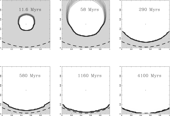
Figure 2: The cross-section of the numerical 3D ionization front going through the source of ionization for a model with no scattering, shown for six output times. The density of the gas follows an exponential gradient (eq. 21) increasing by a factor of $50$ from the upper to the lower side of the cube. The dashed line gives the analytic solution (eq. 22) for an equilibrium Strömgren sphere without scattering. The width of the transition layer between the neutral and fully ionized regions is consistent everywhere with the mean free path of ionizing photons. The ionizing source of luminosity $\dot{N}_{\rm ph}=10^{51}{\rm s}^{-1}$ (all emitted in photons just above the hydrogen Lyman limit) is marked by the asterisk. The nine contour levels correspond to ionization fractions of ${x_{\rm e}}=0.1,0.2,...,0.9$.

Figure 3: In order to cover the whole computational volume with rays uniformly and isotropically, we set the number of rays inside a latitudinal angle interval $[\theta,\theta+d\theta]$ proportional to $\cos\theta$. An odd number of rays will necessarily introduce slight left-right asymmetry for interpolation between the 3D rectangular grid and the radial grid for any non-central cross-section through the volume. In this figure we show a 2D schematic representation of the two grids employed in our method. To simplify the plot, the source of radiation is assumed to be sitting in the centre, and only radial rays are drawn here. Due to the finite angular resolution, interpolation between the 3D mesh and the rays is not symmetric with respect to the centre. This shows up in the asymmetry between the upper and the lower sides of the ionization contours in Fig. 8.

4.3 Ionization in the presence of a UV background

The uniform coverage of the whole volume with rays implies that extended sources of radiation will be represented statistically much better than point sources. A simple test mimicking the evolution of dense clouds in the presence of ionizing radiation is to enclose the computational region in an isotropic bath of photons. The simplest way to accomplish this is just to set up a uniform, isotropically glowing boundary at the edges of the cube at $t=0$. An effective demonstration of time-dependent ray tracing would be its ability to deal with any distribution of state variables within the simulation volume. For this test, we set up a density condensation shaped as the acronym for ‘radiation hydrodynamics’ (RHD), with a density $50$ times that of the ambient homogeneous medium. The ambient medium has a constant density of $\Omega_{\rm b}=10^{-3}$, and the energy density of the background radiation is $E=5\times 10^{-23}\nu_{1}{\rm\,erg}{\rm\,cm}^{-2}{\rm\,Hz}^{-1}{\rm\,sr}^{-1}$. Fig. 4 shows the result of this run. Most of the low-density environment is ionized on the radiation propagation timescale. It takes somewhat longer for ionizing photons to penetrate into the dense regions. Whether these regions can be ionized on a timescale of interest, depends on the ratio of the recombination timescale to the flux of background radiation. One can easily see ionization ‘eating in’ to the neutral zone, e.g. in the disappearance of the serifs on the letters at late times. Note that the width of the ionization fronts does not usually exceed one grid zone (Fig. 5).

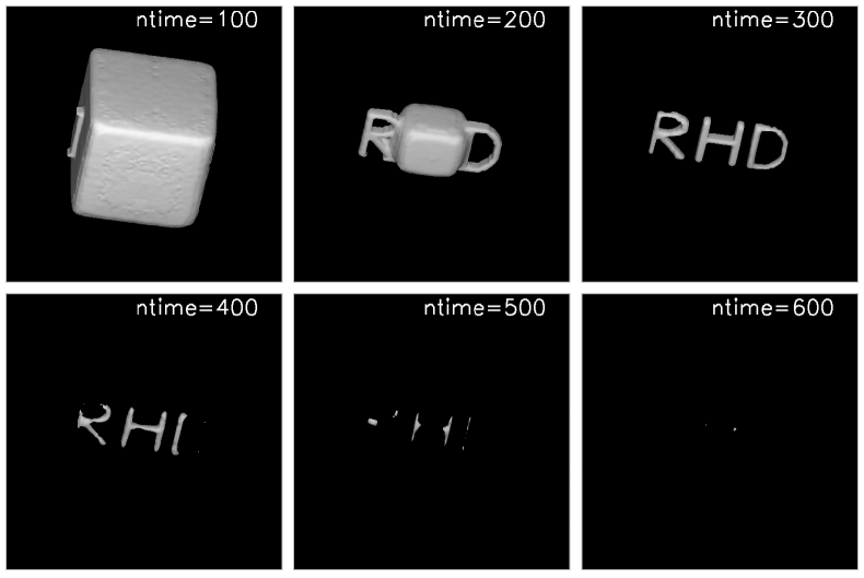
Figure 4: The isosurface of ionization level ${x_{\rm e}}=0.5$ is plotted at six time intervals for the model with an ionizing background coming from outside of the cube. The density contrast between the ambient medium and the high-density acronym ‘RHD’ (radiation hydrodynamics) is $50$. This simulation demonstrates 5D advection on the radiation propagation time-scale. The numerical resolution is $64^{5}$. The effects of shielding are clearly visible during partial ionization.

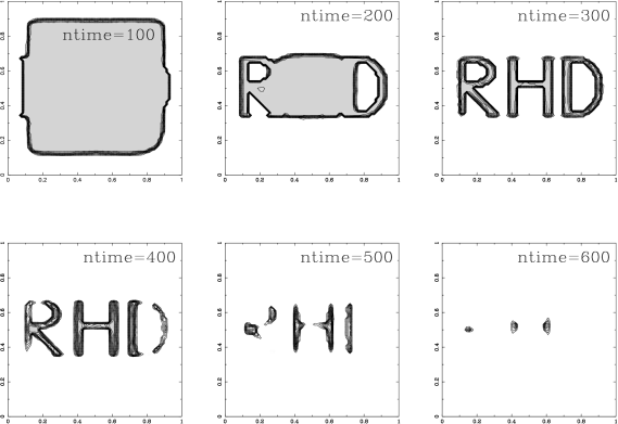
Figure 5: Contour plot of ionization in a cross-section through the data presented in Fig. 4. There are 11 contour lines spaced linearly from ${x_{\rm e}}=0$ to ${x_{\rm e}}=1$. Note the sharpness of the ionization boundaries, the shielding, and the fact that the most deeply embedded regions take the longest to ionize.

4.4 Diffuse radiation from H ii regions: shadows behind neutral clouds

Part of the ionizing radiation at high redshifts comes in the form of hydrogen Lyman continuum photons from recombinations in diffuse ionized regions. The following test, simulating the formation of shadow regions behind dense clouds at the resolution $32^{3}\times 10^{2}$, was adapted from Canto, Steffen & Shapiro (1998). A neutral clump of radius $R_{\rm c}=1.25{\rm\,Mpc}$ (comoving) is being illuminated by a parallel flux $F_{*}=6.34\times 10^{-16}h_{\rm P}^{-1}{\rm\,erg}{\rm\,cm}^{-2}{\rm\,s}^{-1}{\rm\,Hz}^{-1}$ of stellar ionizing photons (just above $13.6{\rm\,eV}$) from one side; here $h_{\rm P}$ is Planck’s constant. A shadow behind the clump is being photoionized by secondary recombination photons from the surrounding H ii region (Fig. 6) of physical density $n_{\rm H}=3.7\times 10^{-2}{\rm\,cm}^{-3}$. Neglecting hydrodynamical effects, the width $R_{\rm I}$ of the shadow region can be estimated using a simple two-stream approximation [Canto et al. 1998]:

$$\xi^{2}={2\over 1+r_{i}^{2}(2\ln r_{i}-1)},~{}~{}~{}{\rm where}~{}~{}~{}r_{i}\equiv{R_{\rm I}\over R_{\rm c}},$$ (23)

and the dimensionless parameter $\xi$ is defined as

$$\xi\equiv{4R_{\rm c}n_{\rm H}^{2}\over F_{*}}{\alpha_{\rm B}^{2}\over\alpha_{1}}.$$ (24)

For $\xi^{2}\leq 2$, recombination Lyman continuum photons from the illuminated region will eventually photoionize the shadow completely. For $\xi^{2}>2$, radiative losses through low-energy cascade recombination photons will stop the I-front, forming a neutral cylinder behind the dense clump. Strictly speaking, equations (23)–(24) are valid only for a shadow completely photoionized by secondary photons, and should be viewed as an approximation to I-fronts driven by scattering.

For this run we modify boundary conditions to include recombination photons originating outside the box. Each of the rays – starting on any face except the upper side of the volume (which goes through the neutral shadow) – carries the additional intensity of $\left\langle\epsilon_{1}\right\rangle/\left\langle\kappa\right\rangle$, where the angular brackets denote the average throughout the currently photoionized gas inside the box.

In Fig. 7 we plot the radius $R_{\rm I}$ of the shadow neutral region as a function of $\xi$ in our 3D numerical models. To play with the size of the neutral core, we fix the total recombination coefficient but we vary the portion of recombinations into the ground state (which would produce more Lyman continuum photons capable of ionizing the medium). The width of the I-front driven by secondary photons depends on the assumed opacity (the optical depth of $\tau=10$ corresponding to the column density of $10^{21}{\rm\,cm}^{-2}$). This low opacity was chosen to reach equilibrium quicker – equilibrium itself does not depend on the opacity – but it cannot be too low otherwise there will be an unnecessary spread of the transition zone in the I-front over many grid cells.

We find a remarkably good agreement between the results of our models and the analytic solution, taking into account that ionization of the shadow is due to scattering in the medium.

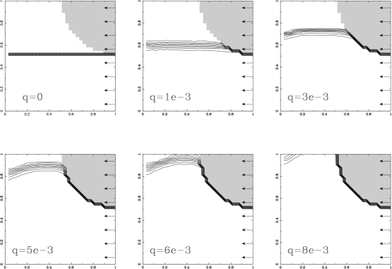
Figure 6: Cross-sections of the dense clump (shaded) and the neutral shadow region behind it, for different fractions $q=\alpha_{1}/\alpha$ of recombination into ground states. The clump is being illuminated with a parallel flux $F_{*}$ of direct stellar ionizing photons entering through one side of the box (marked with arrows), and the shadow region behind it is being photoionized by recombination Lyman continuum photons from the surrounding H ii gas. Each model has been evolved to an equilibrium state, correspoding to many passages of the wavefront across the computational region. The nine contour levels correspond to ionization fractions of ${x_{\rm e}}=0.1,0.2,...,0.9$. This test is adapted from Canto et al. (1998).

Figure 7: The width $R_{\rm I}$ of the shadow behind a neutral clump of radius $R_{\rm c}$ as a function of the dimensionless parameter $\xi$ of eq. (24). The solid line represents the two-stream analytic solution (Canto et al. 1998), assuming an infinitely sharp boundary. The points show the results of our 3D numerical model, plotted explicitly at ${x_{\rm e}}=0.5$, with the errorbars giving the width of the I-front formed by secondary photons. Since the width of the neutral core in our numerical model depends on multiple scatterings in 3D, we would not expect a detailed match; however, the agreement between the approximate analytic and the numerical solutions is remarkably good.

4.5 Diffuse radiation from H ii regions: ionization of a central void

To demonstrate the ability of our scheme to handle scattering in more complicated situations, we also set up a model with ionization of a central low-density void by secondary, recombination photons. The void region is surrounded by two nested cubes with opposite faces open. The walls of the cubes are set to be much denser than the rest of the medium, to screen completely the central void from direct ionizing photons, and the ionizing UV flux is introduced at all faces of the computational volume. The total hydrogen recombination coefficient $\alpha_{1}+\alpha_{\rm B}$ is again taken for the temperature $T=10^{4}{\rm K}$. Similar to Sec. 4.4, we vary the amount of scattering in the medium by changing the fraction $q$ of atoms recombining into the ground state. In reality at $T=10^{4}{\rm K}$ the value $q\approx 0.38$ [Hummer 1994] gives a solution in between our extreme values of $q$.

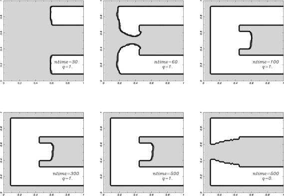
Figure 8: Diagram demonstrating ionization of the void region, which consists of two nested cubes with opposite sides open. The central void and the side ‘tunnels’ have the same density as the surrounding medium, and the density of the walls is set to be much higher to completely block all external ionizing photons. In this figure we plot one of the central cross-sections showing contours of ionization at five different output times for the model with complete scattering ($q=1$), and a quasi-equilibrium configuration for the model with no scattering ($q=0$) after $n=500$ timesteps. The shaded arears represent neutral regions.

Similar to the test problem of Section 4.3, if $\alpha_{\rm B}=0$, then the medium will be ionized completely, since there is a constant flux of primordial ionizing photons. The speed of ionization depends on the values of $\alpha_{1}$, $\alpha_{\rm B}$, $g_{\rm HI}$ and $n_{\rm H}$. Note, however, that if $\alpha_{1}$ is too high, the I-front will be very slow, since a large portion of the original ionizing photons are scattered back. On the other hand, if $\alpha_{1}$ is too low, the I-front will propagate much faster in those regions where ionization is driven by primordial photons, but in shadowed regions there will be too few recombination photons. Thus, it seems that the speed of ionization of the central void will be the highest at some intermediate $\alpha_{1}$.

In Fig. 8 we demonstrate ionization of the void region for models with complete scattering and with no scattering at all. The parameters used for this model are $E=5\times 10^{-20}\nu_{1}{\rm\,erg}{\rm\,cm}^{-2}{\rm\,Hz}^{-1}{\rm\,sr}^{-1}$ and the diffuse neutral gas density $\Omega_{\rm b}=0.01$.

As expected, for the no-scattering model ($q=0$) the central region remains neutral, since there is no direct path for the ionizing photons. However, for the model which includes scattering ($q=1$), at least part of the central region becomes ionized. This demonstrates that our scheme is perfectly capable of dealing with re-scattering of the ionizing photons. Beyond this simple test case, there are many astrophysical situations where progress can be made via numerical radiative transfer. For example, analytic solutions are often used, which are steady-state, and which assume a sharp boundary between the neutral and ionized zones. Using our numerical techniques it should be possible to follow general systems with complex density inhomogeneities as well as regions of partial ionization.

5 Conclusions

In this paper we have demonstrated that, with existing desktop hardware, it is possible to model cosmological inhomogeneous reionization on a light-crossing time $t_{\rm R}$ in three spatial dimensions. Since the photoionization time-scale in the low optical depth regime ($\tau\leq 1$) is of order of the light-crossing time $t_{\rm R}$, explicit advection might be a faster method in covering at least these regions. Compared to the elliptic-type solvers on the fluid-flow time-scale or the time-scale of atomic processes, explicit radiative advection produces very accurate results without the need to solve a large system of coupled non-linear elliptic equations. The computing requirements with explicit advection grow linearly with the inclusion of new atomic and molecular rate equations, which is certainly not the case for quasi-static solvers (although it is feasible that the development of multigrid techniques for elliptic equations might actually approach similar scaling).

Using eq. (1) we can see that the entire history of reionization can be modeled with $\sim 10^{4}$–$10^{5}$ time-steps (depending on the required resolution), which makes explicit advection an attractive choice for these calculations. However, the efficiency of the explicit radiative solver has still to be explored. Future work should include a detailed comparison between explicit advection and implicit reconstruction (through an elliptic solver), to demonstrate which method works best for calculating inhomogeneous reionization.

As we have demonstrated here, for certain problems, including the propagation of supersonic I-fronts, the Courant condition does not seem to impose prohibitively small time-steps. In this case the biggest challenge is to accurately describe anisotropies in the radiation field, i.e. to solve for inhomogeneous advection in the 5D phase space, in the presence of non-uniform sources and sinks of radiation. Strictly speaking, the storage of one variable at, say, $64^{5}$ data points requires about $9\,$GB of memory, which stretches the capabilities of top-end desktop workstations. One attractive possibility for future exploration is to directly solve the monochromatic photon Boltzmann equation in 5D. To demonstrate the feasibility of the numerical solution, however, among different methods, we here chose to concentrate on simple ray tracing at the speed of light. The numerical approach we have used is completely conservative and produces very little numerical dissipation.

We want to conclude that despite the high dimensionality of the problem, with a reasonable expenditure of computational resources, of the type available today, it is possible to numerically model many different aspects of the full 3D radiative transfer problem. Furthermore we feel that the methods described here represent a significant and realizable step towards the goal of full cosmological RHD.

References

- [Abel et al. 1997] Abel T., Anninos P., Zhang Y., Norman M.L., 1997, New Astronomy, 2, 181
- [Abel et al. 1998] Abel T., Norman M.L., Madau P., 1998, astro-ph/9812151
- [Anninos et al. 1997] Anninos P., Zhang Y., Abel T., Norman M.L., 1997, New Astronomy, 2, 209
- [Auer & Mihalas 1970] Auer L.H., Mihalas D., 1970, MNRAS, 149, 65
- [Canto et al. 1998] Canto J., Steffen W., Shapiro P.R., 1998, ApJ, 502, 695
- [Couchman & Rees 1986] Couchman H.M.P., Rees M.J., 1986, MNRAS, 221, 53
- [Evans 1998] Evans F., 1998, J. Atmospheric Sciences, 55, 429
- [Gnedin & Ostriker 1997] Gnedin N.Y., Ostriker J.P., 1997, ApJ, 486, 581
- [Haiman & Loeb 1997] Haiman Z., Loeb A., 1997, ApJ, 483, 21
- [Haiman & Loeb 1998] Haiman Z., Loeb A., preprint astro-ph/9710208
- [Hummer 1994] Hummer D.G., 1994, MNRAS, 268, 109
- [Katz et al. 1996] Katz N., Weinberg D.H., Hernquist L., Miralda-Escudé J., 1996, ApJ, 457, L57
- [Kepner et al. 1997] Kepner J.V., Babul A., Spergel D.N., 1997, ApJ, 487, 61
- [Madau et al. 1997] Madau P., Meiksin A., Rees M.J., 1997, ApJ, 475, 429
- [Madau 1998] Madau P., 1998, preprint astro-ph/9807200
- [Meiksin 1994] Meiksin A., 1994, ApJ, 431, 109
- [Mihalas & Mihalas 1984] Mihalas D., Mihalas B., 1984, Foundations of Radiation Hydrodynamics. Oxford University Press, New York
- [Miralda-Escudé 1998] Miralda-Escudé J., Haehnelt M., Rees M.J., 1998, astro-ph/9812306
- [Navarro & Steinmetz 1997] Navarro J.F., Steinmetz M., 1997, ApJ, 478, 13
- [Norman et al. 1998] Norman M.L., Paschos P., Abel T., 1998, astro-ph/9807282
- [Park & Hong 1998] Park Y.-S., Hong S.S., 1998, ApJ, 494, 605
- [Shapiro 1986] Shapiro P.R., 1986, PASP, 98, 1014
- [Shapiro et al. 1998] Shapiro P.R., Raga A.C., Mellema G., 1998, preprint astro-ph/9804117
- [Spitzer 1968] Spitzer L., Jr., 1968, Diffuse matter in space. Interscience publishers, New York
- [Stone & Mihalas 1992] Stone J.M., Mihalas D., 1992, JComputPhys, 100, 402
- [Stone et al. 1992] Stone J.M., Mihalas D., Norman M. L., 1992, ApJS 80, 819
- [Tajiri & Umemura 1998] Tajiri Y., Umemura M., 1998, preprint astro-ph/9806046
- [Umemura et al. 1998] Umemura M., Nakamoto T., Susa H., 1998, in Miyama S. M., Shibata K., eds, Numerical Astrophysics 1998. Kluwer, in press
- [Zhang et al. 1998] Zhang, Y., Meiksin, A., Anninos, P., Norman, M.L., 1998, ApJ, 495, 63