RXTE Observation of Cygnus X–1: III. Implications for Compton Corona and ADAF Models

Abstract

We have recently shown that a ‘sphere+disk’ geometry Compton corona model provides a good description of Rossi X-ray Timing Explorer (RXTE) observations of the hard/low state of Cygnus X–1. Separately, we have analyzed the temporal data provided by RXTE. In this paper we consider the implications of this timing analysis for our best-fit ‘sphere+disk’ Comptonization models. We focus our attention on the observed Fourier frequency-dependent time delays between hard and soft photons. We consider whether the observed time delays are: created in the disk but are merely reprocessed by the corona; created by differences between the hard and soft photon diffusion times in coronae with extremely large radii; or are due to ‘propagation’ of disturbances through the corona. We find that the time delays are most likely created directly within the corona; however, it is currently uncertain which specific model is the most likely explanation. Models that posit a large coronal radius [or equivalently, a large Advection Dominated Accretion Flow (ADAF) region] do not fully address all the details of the observed spectrum. The Compton corona models that do address the full spectrum do not contain dynamical information. We show, however, that simple phenomenological propagation models for the observed time delays for these latter models imply extremely slow characteristic propagation speeds within the coronal region.

1. Introduction

In a previous paper (Dove et al. (1998), hereafter paper I) and in a companion paper to this work (Nowak et al. (1998a), hereafter paper II) we have presented analysis of a 20 ksec Rossi X-ray Timing Explorer (RXTE) observation of the black hole candidate Cygnus X–1. Using self-consistent numerical models of a hot spherical corona surrounded by a cold, geometrically thin disk, we were able to describe successfully the spectrum of Cyg X–1 over a broad range in energy, $3$–$200$ keV (paper I; see also Dove et al. (1997)). We derived an optical depth for the spherical corona of $\tau=1.6\pm 0.1$ and an average temperature of $kT=87\pm 5$ keV (reduced $\chi^{2}$ for the fit was 1.56; paper I).

Timing analysis (paper II) showed that our observation of the hard state of Cyg X–1 was similar to previous hard state observations of this object (Miyamoto & Kitamoto (1989); Belloni & Hasinger (1990a, b); Miyamoto et al. (1992)); however, we were able to extend our analysis to a decade lower in Fourier frequency and half a decade higher in Fourier frequency as compared to most previous observations. Cyg X–1 showed root mean square (rms) variability $\approx 30\%$ characterized by a power spectral density (PSD) that was nearly flat between $0.02$–$0.2$ Hz. The PSD was approximately $\propto f^{-1}$ between $\approx 0.2$–$2$ Hz, while the power law index of the $2$–$90$ Hz PSD was seen to increase from $\approx-1.7$ to $\approx-1.4$ between the lowest and highest energy bands. The coherence function, rarely presented for most previous observations (although see Vaughan (1991); Vaughan & Nowak (1997); Cui et al. (1997)), was remarkably close to unity over a wide range of frequencies. We also considered the Fourier frequency-dependent time delay between soft and hard photons.

As discussed in paper II, hard photons in Cyg X–1 are seen to lag behind soft photons with a time delay that is dependent upon Fourier frequency (see also Miyamoto & Kitamoto (1989); Miyamoto et al. (1992); Cui et al. (1997); Crary et al. (1998)). Comparing the ($0$–$3.9$ keV) band to the ($14.1$–$45$ keV) band, the time delays are approximately $\propto f^{-0.7}$ and range from $\approx 2\times 10^{-3}$–$0.05$ s. A more detailed study of these time delays will be the focus of this work. Specifically, we wish to understand what leads to this factor of $20$ range in timescales, and we consider models where the time lags are: created within the outer accretion disk (§2); created via photon diffusion in an extremely large corona (§3); or are due to wave propagation (§4).

As the basis for our discussions, we will for the most part take as our straw man model the ‘sphere+disk’ Comptonization model that we considered in paper I. We illustrate the geometry of this model in Figure 1. This model has a uniform coronal heating rate, nearly uniform density structure, but a non-uniform temperature structure. The seed photons for Comptonization are due to (reprocessed and direct) soft radiation from the outer, thin disk. This model does not include dynamical information. The Advection Dominated Accretion Flow (ADAF) models have a similar geometry, as shown in Figure 1, but they model the accretion dynamics as well (Abramowicz et al. (1995); Narayan & Yi (1994); Narayan (1996); Esin, McClintock & Narayan (1997)). For ADAFs, a substantial portion of the accretion energy is advected into the black hole, potentially at a large fraction of free-fall speeds, in the form of thermal energy. (The density profile of matter in free-fall is $\propto R^{-3/2}$.) The advective inner regions also produce cyclo/synchrotron photons, which are assumed to be the seed photons for Comptonization. Another model that we shall discuss is the Comptonization model of Kazanas, Hua & Titarchuk (1997), hereafter referred to as KHT (see also Boetcher & Liang (1998)). This model postulates a large spherical corona with a radial density profile typically $\propto R^{-3/2}\rightarrow R^{-1}$, but uniform temperature structure. The seed photons for Comptonization are isotropic and can originate either within the central regions of the corona (KHT), or externally (Boetcher & Liang (1998)). Note that these models do not consider detailed flow dynamics.

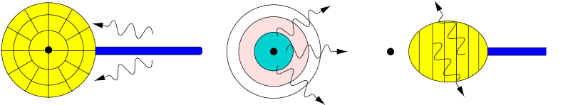
Figure 1.— Geometries for recent models of Cyg X–1 . Left: Sphere+disk geometry, as considered by Dove et al. (1998) (paper I). The seed photons for Comptonization come from the outer disk. The central corona has a uniform heating rate and seed electron density but a non-uniform temperature structure. (cf. Dove, Wilms, & Begelman 1997). Middle: Geometry considered by Kazanas, Hua, & Titarchuk (1997). The seed photons for Comptonization are isotropic and arise from an unspecified source within the central region of the system. The corona has a spherical structure with a typically $R^{-3/2}\rightarrow R^{-1}$ density profile, but uniform temperature structure. Right: Advection Dominated Accretion Flow (ADAF) geometry (cf. Narayan 1996). The seed photons for Comptonization are cyclo/synchrotron photons that originate within the advective inner region. A cylindrical symmetry approximation for the structure is often taken.

In order to understand how these models might lead to the observed time delays, let us consider some of their characteristic timescales. We shall take the fiducial radius of the corona (or inner, advective region) to be $R=50~{}GM/c^{2}$, with $M=10~{}M_{\odot}$. (We shall adopt $M=10~{}M_{\odot}$ throughout the rest of this paper.) We then have the following characteristic timescales. The radial light-crossing timescale, $t_{\rm LC}$, is $2.5\times 10^{-3}$ s, which is comparable to the shortest time lags. For an 87 keV Compton corona the radial sound crossing time, $t_{\rm SC}=5\times 10^{-3}$ s. The free-fall timescale, $t_{\rm FF}$, relevant for the ADAF models, is $8.5\times 10^{-3}$ s and is proportional to $R^{3/2}$. All three of these timescales are mainly relevant for the shortest time delays. In order for them to be applicable to the longest time delays, one needs to consider a radius of $10^{3}~{}GM/c^{2}$ for the light-crossing timescale and a radius of $\approx 160~{}GM/c^{2}$ for the free-fall timescale. (Some ADAF models do posit a large radius for the advective region; Narayan (1996); Esin, McClintock & Narayan (1997).) A single one of these mechanisms can explain the observed dynamic range in time delays only if it samples a comparably large range in radii.

The viscous diffusion timescale is $\approx R^{2}/\nu$, where $\nu$ is the kinematic viscosity. Taking an $\alpha$-disk model, $\nu\approx\alpha Hc_{s}$, where $H$ is the disk thickness, and $c_{s}$ is the speed of sound (cf. Frank, King & Raine (1992)). Using the speed of sound from our best fit corona model and taking $H\approx R$ and $\alpha\approx 0.1$, the viscous diffusion time, $t_{\rm D}$, is approximately $0.03$ s, which is comparable to the longest time lags. The Keplerian period at $R=50~{}GM/c^{2}$ is $t_{\rm K}\approx 0.1$ s, and is also comparable to our longest time delays. All of the above characteristic timescales, along with the observed time lags, are presented in Figure 2.

We see that there are a range of characteristic timescales comparable to both the shortest and longest observed time lags. The latter are perhaps the more difficult to understand theoretically. Two extremes for explaining the longest time lags are: a small radius and a slow mechanism (e.g., viscous diffusion); or a fairly large radius and a fast mechanism (e.g., light or sound speed propagation). The fact that there is extremely high coherence between the soft and hard bands (cf. paper II), even at frequencies near $0.1$ Hz where we see the longest time delays, makes it unlikely that a combination of these two possibilities is at work. (Even individually coherent processes will appear incoherent when summed, unless each process yields the same transfer function from soft to hard; Vaughan & Nowak (1997)).

Figure 2.— RXTE observations of time delays between the ($0$–$3.9$ keV) and ($14.1$–$45$ keV) lightcurves of Cyg X–1. Diamonds indicate where the hard lags the soft, and stars indicate where the soft lags the hard (paper II). Lines represent characteristic timescales for a coronal radius of $50~{}GM/c^{2}$ with $M=10~{}M_{\odot}$. Solid line is the radial light crossing timescale ($t_{\rm LC}$); long dashed line is the radial sound crossing time ($t_{\rm SC}$); short dashed line is the free-fall timescale ($t_{\rm FF}$); dash dot line the viscous diffusion timescale for a hot, geometrically thick cloud ($t_{\rm D}$); and the dash triple dot line is the Keplerian orbital period for a thin disk ($t_{\rm K}$).

In this paper, we consider both of the above possibilities. In section 2 we calculate the effect that coronal ‘reprocessing’ has on time delays that are intrinsic to the soft X-ray seed photons. We explore this possibility, first discussed by Miller (1995) and Nowak & Vaughan (1996), using our best-fit coronal model of paper I. In section 3, we consider the suggestion of KHT that the time delays are created by Compton scattering in a corona that extends several decades in radius. We present simple, phenomenological propagation models in section 4. We use these models to show that the time delays can have a complicated frequency dependence even under very simple assumptions. We furthermore discuss the characteristic propagation speeds that such models imply. We present our conclusions in section 5.

2. Time Delays Intrinsic to the Seed Photons

As discussed in paper II (and references therein), one naturally expects that the hard photons lag the soft photons if the high energy spectrum is mainly due to Comptonization. The time delay is due to the fact that the hard photons undergo several more scattering events than the soft photons. Such time delays should approximately depend upon the logarithm of the energy (paper II, and references therein), and should be of order the light crossing time of the corona. As was first pointed out by Miyamoto & Kitamoto (1989), and shown in Figure 2 above, this is considerably shorter than the longest observed delays.

This fact led Miller (1995) to suggest that the time lags might be intrinsic to the seed photons for Comptonization, and that the input time delay’s frequency dependence (although not amplitude) might be preserved by Comptonization. As discussed by Miller (1995) and elaborated upon by Nowak & Vaughan (1996), the Fourier frequency-dependence of the time delay is preserved, typically at low frequency, if the difference between the input and output photon energies is not too great. The amplitude of the time delay, however, tends to be decreased in the scattering process, perhaps substantially so (Nowak & Vaughan (1996)). A constant time delay is introduced typically at high Fourier frequency. The amplitude of this time lag ‘shelf’ is given by the difference of the mean diffusion times through the Compton cloud for the two energy bands being compared, and thus should depend logarithmically upon energy (Pozdnyakov, Sobol & Sunyaev (1983); Miller (1995); Nowak & Vaughan (1996)). In addition to the introduction of a constant time delay at high Fourier frequency, one also expects that the intrinsic PSD of the seed photons will be attenuated, especially at high frequency (Brainerd & Lamb (1987); Kylafis & Klimis (1987); Wijers, van Paradijs & Lewin (1987); Stollman et al. (1987); Bussard et al. (1988); Kylafis & Phinney (1989); Miller & Lamb (1992); Miller (1995); Nowak & Vaughan (1996)).

Given a source of seed photons and a Comptonization model, one can calculate these effects (Miller (1995); Nowak & Vaughan (1996)). Take a discretely sampled seed photon lightcurve, $s_{i}^{[k]}$, where $i$ denotes the time bin and $[k]$ denotes the energy band. The output lightcurve, $h_{j}^{[l]}$, is measured at times $j$ and in energy band $[l]$. The two can be related by an equation of the form

$$h_{j}^{[l]}~{}=~{}\sum_{k}r_{ji}^{[lk]}s_{i}^{[k]}~{}~{},$$ (1)

where $r_{ji}^{[lk]}$ describes the linear transfer properties of the Comptonizing medium in both time ($i\rightarrow j$) and energy ($[k]\rightarrow[l]$) (cf. Nowak & Vaughan (1996), and the Appendix below). The Compton corona can be described by such a linear transfer function if the coronal structure is stationary, which would also imply a unity coherence function measured between the output bands (Nowak & Vaughan (1996)).

In Fourier space, eq. (1) can be written as

$$H_{m}^{[l]}~{}=~{}\sum_{k}R_{m}^{[lk]}S_{m}^{[k]}~{}~{},$$ (2)

where capital letters denote discrete Fourier transforms, $m$ denotes the discrete frequency bin, and $R_{m}^{[lk]}$ is the transform of a column of $r_{ji}^{[lk]}$ (i.e., $i$ held fixed and $j$ free to vary; Nowak & Vaughan (1996)). We can then relate the measured PSD and cross power spectrum (CPD) to the input PSD and CPD by

$${H_{m}^{[l]}}^{\ast}H_{m}^{[n]} = \sum_{k}{R_{m}^{[lk]}}^{\ast}R_{m}^{[nk]}\left(S_{m}^{[k]}\right)^{2}$$ (3)

$$+\sum_{j\neq k}{R_{m}^{[lk]}}^{\ast}R_{m}^{[nj]}\left({S_{m}^{[k]}}^{\ast}S_{m}^{[j]}\right)~{}~{}.$$

Given a Comptonization model we can readily calculate $r_{ji}^{[lk]}$, which can then easily be Fourier transformed to yield $R_{m}^{[lk]}$. As described in the Appendix, we have calculated the transfer functions for our best fit Comptonization model of paper I. We use these transfer functions to assess the effect of our Compton corona model on an input white noise source with an intrinsic time delay between soft and hard photons that is $\propto f^{-1}$. In our model of paper I, $25\%$ of the seed photons come from energies $<40.4$ eV, $50\%$ come from energies $<115$ eV, and $75\%$ come from energies $<214.4$ eV. We choose these three energies as seed photon energies, and furthermore we impose a constant Fourier phase lag of $\pi/2$ between the $214.4$ eV and $115$ eV variability, as well as between the $115$ eV and $40.4$ eV variability. The resulting phase lag of $\pi$ between the $214.4$ eV and $40.4$ eV variability is the maximum allowed phase lag between any two energy bands (see Nowak & Vaughan (1996), and paper II). We also choose the amplitude of the variability to be identical for all three seed photon energy bands.

In Figure 3 we present the result of passing such white noise variability through our Comptonization model of paper I. As an example, we present theoretical time delays and PSD for the ($2$–$4$ keV) band compared to the ($12$–$50$ keV) band. (Neutral hydrogen column density is not included in these theoretical calculations of time delays.) We hold all parameters of the Comptonization model fixed, including the temperature of the seed photons from the disk, to the values of paper I; however, we vary the physical radius of the corona. Specifically, we consider radii of $30~{}GM/c^{2}$, $50~{}GM/c^{2}$, $150~{}GM/c^{2}$, and $500~{}GM/c^{2}$. A number of results are immediately apparent from these figures.

First, the largest physically allowed phase lag between the $214.4$ eV and $40.4$ eV variability was still too small to reproduce the majority of the observed time delays. Thus the hypothesis of Miller (1995) and Nowak & Vaughan (1996) that the time delays could be intrinsic to the disk appears to be wrong. As discussed by Nowak & Vaughan (1996), such a large input phase lag is required because of the great disparity between the input energy ($\approx 150$ eV) and the output energies ($\approx 3$ keV, $20$ keV). The required input phase lag can be decreased if the temperature of the seed photons is increased; however, this is not allowed by the energy spectral modeling (paper I). Further argument against the hypothesis is garnered from the fact that the calculated time delays do not depend logarithmically upon energy, contrary to the observations (paper II, and references therein). The theoretical model does show a logarithmic energy dependence at high Fourier frequency, where a shelf in the theoretical time delay is clearly seen; however, the energy dependence weakens for lower frequencies. As shown in paper II (Figure 12), the data show a logarithmic energy dependence even at $0.3$ Hz. We are thus forced to the conclusion that the majority of the observed time delays, in one fashion or another, must be created within the corona if our basic model for the energy spectrum is correct. However, this is not the same as saying that the variability (PSD) must be directly created in the corona (cf. §3).

We do expect one effect of Comptonization to remain, even if the time lags are created within the corona itself, namely the time lag shelf at high frequency. After one scatter, a photon has essentially lost all information as to the spatial location of its origin. Thus whether the seed photons come from an outer disk or whether they are internal to the corona (such as for ADAF models that invoke cyclo/synchrotron seed photons; Narayan (1996); Esin, McClintock & Narayan (1997)), the difference in diffusion times to reach two different output energies will still lead to a time lag shelf. The shortest observed time lag should be no smaller than this theoretically expected shelf. Such shelves clearly are seen at high Fourier frequency in the theoretical models presented in Figure 3. They range from $2\times 10^{-3}$ s for $R=30~{}GM/c^{2}$ to $0.04$ s for $R=500~{}GM/c^{2}$. The observational data, on the other hand, do show a flattening in the time delays in the $10$–$30$ Hz range. If we take this as the upper limit to an allowed theoretical time delay, then the maximum allowed coronal radius for our model of paper I is $\approx 30~{}GM/c^{2}$. There is also an observed flattening of the time delay in the region of $0.7$–$3$ Hz. If we take this as the upper limit to an allowed theoretical time delay, then the maximum allowed coronal radius is $\approx 150~{}GM/c^{2}$.

Which of these observational limits should we choose, and why do we ignore the even shorter time delays above $30$ Hz? As discussed in paper II, the time delays above $30$ Hz are especially subject to noise as both the PSD and the coherence function are decreasing in this regime. We again note that there is a ‘hardening’ of the $2$–$90$ Hz PSD with increasing energy (paper II), coincident with this coherence loss. We postulated that this was indicative of additional, multiple variability components that were being created directly within the corona. One speculation would be that these timescales are probing flares that are ‘feeding’ the corona on dynamical timescales. Without being able to identify the physical nature of these hypothesized extra variability components, we do not know what their intrinsic time delays are. We do know, however, that multiple uncorrelated variability components will lead to a loss of coherence, and that the net observed time delay in such regions will be a combination of many intrinsic lags and possibly even leads (Vaughan & Nowak (1997); paper II, §3.1). Thus an incoherent frequency range can have observed time delays less than the minimum theoretically expected time lag shelf.

We should then choose the maximum allowed theoretical time lag shelf to be the minimum time delay observed in a region of near unity coherence. For our observations of Cyg X–1, this would be at $\approx 10$ Hz, and thus this limits us to a maximum coronal radius of $\approx 30~{}GM/c^{2}$. This is consistent with the limits on the PSD as well (cf. Figure 3). Such a small corona has little effect on the PSD in the $0.02$–$2$ Hz regime, where PSD for all five observed energy bands (paper II) have roughly the same shape. We note, however, that based upon the PSD alone, especially if the PSD above $\mathrel{\hbox to0.0pt{\raise 2.20013pt\hbox{$>$}\hss}{\lower 2.20013pt\hbox{$\sim$}}}10$ Hz is contaminated by other sources of variability, a much larger coronal radius ($\approx 150~{}GM/c^{2}$) is tolerated.

It is tempting to associate the various ‘flattened’ regions ($\approx 0.1$–$0.5$ Hz, $\approx 0.7$–$3$ Hz, and $\approx 10$–$30$ Hz) seen in the time delays of Figure 3 with time lags shelves due to Comptonization. This would imply a Compton corona with characteristic radii of $\approx 30~{}GM/c^{2}$, $\approx 150~{}GM/c^{2}$, and $\approx 500~{}GM/c^{2}$. The (nearly) uniform density coronal model of paper I cannot produce such a range of time lags. However, recently KHT have proposed a coronal model with an $R^{-1}$ density profile that can produce a broad dynamic range of time delays. We consider such models in the next section.

Figure 3.— Left: Diamonds and stars are the same time lags as shown in Figure 2. Solid lines are the theoretical time delays between the ($12$–$50$ keV) and ($2$–$4$ keV) lightcurves, assuming that the seed photons for Comptonization have an intrinsic phase lag of $\pi$ between the 40.4 eV and 214.4 eV lightcurves. (The intrinsic time lag in the seed photons is therefore $\propto f^{-1}$; see text.) Right: Diamonds are the observed Cyg X–1 PSD in the ($14.1$–$45$ keV) band, compared to theoretical ($12$–$50$ keV) PSD for a white noise input (arbitrary normalization). For both figures, the solid line represents a coronal radius of $R=30~{}GM/c^{2}$, the long dashed line represents $R=50~{}GM/c^{2}$, the short dashed line represents $R=150~{}GM/c^{2}$, and the dash dot line represents $R=500~{}GM/c^{2}$.

3. Time Delays Created by the Corona

In the model of KHT, as well as the models of Boetcher & Liang (1998), both the observed power spectral densities and time lags are the result of passing an isotropically emitted white noise (i.e. flat) spectrum through an extended Comptonizing medium with a power-law density profile. The case of $\rho\propto R^{-1}$ represents equal optical depth per decade of radius, and therefore roughly equal probability of seed photons from an isotropic source scattering within any given radial decade. This leads to a power-law shape for the observed PSD, as opposed to the fairly sharp cutoff seen in Figure 3. Time delays are created by the difference in diffusion times through the corona for hard and soft photons. Photons that scatter over large radii will have their intrinsic high frequency variability wiped out (as in Figure 3); therefore, any observed high-frequency variability must be due to photons that scattered only within the inner radial regions. High frequency variability thus exhibits short time delays between hard and soft photons. Low frequency variability potentially can be observed from photons that have scattered over large radius. Low frequency variability thus exhibits longer time delays between hard and soft photons. The time delay at all Fourier frequencies is expected to increase as the logarithm of the ratio of the hard to soft energy, as is observed (cf. paper II, and references therein). For quantitative agreement with the observations, KHT require coronal radii of ${\cal O}(10^{4}~{}GM/c^{2})$.

The main objection to this scenario is that the source of soft seed photons is not fully specified. ASCA observations of the hard/low states of Cyg X–1 (Ebisawa et al. (1996)) and of GX339–4 (Wilms et al. 1998, in preparation) show evidence of a ‘soft excess’ that is reasonably well-modeled by a multicolor blackbody spectrum with a peak temperature of $\sim 150$ eV. This temperature is suggestive of— but not definitive evidence for— the inner edge of an accretion disk (the putative source of the seed photons, although see Narayan (1996); Esin, McClintock & Narayan (1997)) being at radii $\mathrel{\hbox to0.0pt{\raise 2.20013pt\hbox{$>$}\hss}{\lower 2.20013pt\hbox{$\sim$}}}50~{}GM/c^{2}$, as opposed to being at the center of the corona. Both of these sources, as well as several other low/hard state GBHC have shown evidence of weak and narrow Fe lines at 6.4 keV (Ebisawa et al. (1996); Wilms et al. 1998, in preparation). The properties of these lines can be explained naturally in the sphere+disk geometry.

Figure 4.— Best fit ‘sphere+disk’ Comptonization model to RXTE data of Cyg X-1. (Circles are PCA data, triangles and squares are HEXTE data; cf. paper I.) Unlike the Comptonization models presented in paper I, here the heating rate per particle is $\propto R^{-1}$ and the coronal density structure is $\propto R^{-1}$. The best fit parameters were a total optical depth of 2.9 and an average coronal temperature of 58 keV. The reduced $\chi^{2}$ for the fit was 1.75. As discussed in paper I, a possible reason for the residuals in the 3–7 keV region (which are slightly larger than the systematic uncertainties in the PCA) is our assumption of a sharp transition from thin, cold disk to thick, hot corona.

Does a corona with a power law density profile, but with seed photons arising from a geometrically thin outer disk, still produce the characteristic PSD and time delays as described by KHT? To answer this question, we have created a grid of Comptonization spectra with the following properties. The heating per particle in the corona was taken to go as $R^{-1}$ (i.e., proportional to gravitational energy release), the density was taken to go as $R^{-1}$ (i.e., the density structure chosen by KHT), and the seed photons were taken to come from a multicolor blackbody spectrum, with peak temperature 150 eV, originating from a geometrically thin outer disk. We used the same Comptonization code as described in Dove, Wilms & Begelman (1997) and used in paper I. Unlike the models of KHT, which were isothermal out ${\cal O}(10^{4}~{}GM/c^{2})$, our simulations include the derivation of the self consistent temperature structure of the corona by balancing the local Compton cooling rate with the local heating rate (which was $\propto R^{-1}$). For typical parameter values, the temperature was about 72 keV above the pole of the corona, and only 40 keV at the equator near the edge of the sphere. (This cooler temperature is due to the increased density of soft photons near the accretion disk.) We applied these models to our RXTE spectra of Cyg X–1 (cf. paper I), and obtained a reasonable fit to the data (Fig. 4). We find a best fit coronal optical depth of 2.9, with an average coronal temperature of 58 keV.

As described in the Appendix, we again used a linear Monte Carlo code (with the radial coronal structure taken from our best fit nonlinear model, but excluding the pole to equator temperature gradient) to calculate the time-dependent transfer functions for seed photon energies to transit to observed hard X-ray energies. In an analogous manner to the calculation described in §2, we used these transfer functions to determine the effect that the corona has on any variability inherent to the Comptonization seed photons. In Figure 5a, we show the resulting time lags between soft and hard X-ray variability. In Figure 5b, we show the resulting PSD assuming a white noise power spectrum for the variability of the seed photons. Here we take all the photons, an input blackbody with temperature $kT=150$ eV, to have a uniform initial Fourier phase. In both of these figures, we present results for coronal radii ranging from 30–$500~{}GM/c^{2}$.

Note that unlike the models of KHT and Boetcher & Liang (1998), we do not find time lags that are proportional to Fourier period and we do not find a PSD with a power law dependence over a wide range of frequencies. Our results are qualitatively and quantitatively similar to the uniform (in density and heating) coronal models presented in Figure 3. Specifically, the resulting time lag is nearly constant as a function of Fourier frequency, and is comparable to the light crossing time across the diameter of the entire corona. The resulting PSD (assuming a white noise input) has a sharp cut-off as opposed to a power law shape.

The major difference between the model presented here and those of KHT and Boetcher & Liang (1998) is one of geometry. The latter models assume an isotropic source of seed photons. The models of KHT assume that the seed photons originate from interior to the corona, while the models of Boetcher & Liang (1998) consider both internal and external illumination of the corona. Both models, assume isotropic illumination. The core of the corona, where the photons can undergo the scatters on the shortest timescales and thus not suffer substantial losses of high frequency variability power, is initially visible to the seed photons in these models.

In our model, where the seed photons originate in a geometrically thin disk exterior to the corona, the central core of the corona subtends a very small solid angle as viewed by the disk. The photons emanating from the disk do not isotropically illuminate the corona. This geometry, coupled with the fact that our best-fit model is mildly optically thick, means that a substantial fraction of the photons must first scatter on the large radii of the outer corona before being able to scatter within the inner radii of the corona. Thus the time lags are dominated by the longest time delays at all Fourier frequencies.

Further differences with our model are that we consider coronal heating $\propto R^{-1}$, we allow reprocessing of hard X-ray photons in the geometrically thin, outer accretion disk, and we allow for anisotropic temperatures in the corona (although in the linear Monte Carlo code we only include the radial temperature gradients). We conjecture that the primary reason the results of KHT (who use a uniform coronal temperature of $50$ keV and optical depth of $\tau=2$) are so drastically different is precisely because of their choice of an isotropic source of seed photons. [Boetcher & Liang (1998) show that results qualitatively similar to those of KHT are obtained even if the isotropic source of seed photons is exterior to the corona.] Again, the physical nature of this source is not fully described in the work of KHT. However, such a seed photon source geometry is qualitatively similar to that predicted by ADAF models (Narayan (1996); Esin, McClintock & Narayan (1997)). In our model the seed photons only ‘isotropize’ (as viewed by the corona) after scattering on large radii, and therefore always exhibit the longest time delays.

Figure 5.— Left: Diamonds and stars represent the same time lags as shown in Figure 2. Lines are the theoretical time delays between the ($14.1$–$45$ keV) and ($1$–$3.9$ keV) lightcurves assuming that the seed photons originate in the geometrically thin outer disk and have a temperature of $kT=150$ eV. Right: Diamonds are the observed Cyg X–1 PSD in the ($14.1$–$45$ keV) band. Lines are the theoretical PSD for the ($14.1$–$45$ keV) band assuming that the $kT=150$ eV seed photons have a white noise power spectrum (arbitrary normalization). For both figures, the solid line represents a coronal radius of $R=30~{}GM/c^{2}$, the long dashed line represents $R=50~{}GM/c^{2}$, the short dashed line represents $R=150~{}GM/c^{2}$, and the dash dot line represents $R=500~{}GM/c^{2}$.

4. Propagation Models

It has been suggested that the observed variability in Cyg X–1 can be produced in the context of ADAF models by disturbances propagating from the cold, outer disk into the hot, advection-dominated inner region (Manmoto et al. (1996)). Manmoto et al. (1996) considered the inward propagation, and advection, of a large-amplitude, cylindrically symmetric disturbance. The basic concept of an inward propagating wave presented in Manmoto et al. (1996) is an intriguing one. If the cold outer disk, which is not directly observed by RXTE, is the source of disturbances and the inner region then responds to these disturbance in a linear fashion, then we expect there to be unity coherence between hard and soft photons (Vaughan & Nowak (1997)). As also discussed by Vaughan & Nowak (1997), two-dimensional waves can reproduce some of the qualitative features of the observed time delays.

The work of Manmoto et al. (1996) was not directly applicable to Cyg X–1, however, as it only considered modulation of the thermal bremsstrahlung emission, which is essentially negligible in ADAF models; it did not quantitatively address the lags between hard and soft X-ray photons; and their model only produced modulation on order of the advective timescale, and not on the broad range of timescales required to explain the Cyg X–1 PSD. The basic concept, however, is worth considering further. Lacking a dynamical theory associated with our Comptonization models, we explore below the notion of propagating disturbances via the use of simple phenomenological models.

We consider two-dimensional waves not only because they are naturally suggested by a disk geometry (i.e., the hypothesized source of disturbances), but also because even in the absence of any dispersive mechanisms, two-dimensional waves do not satisfy Huygen’s principle (cf. Morse & Feshbach (1953)). This means that even in a nondispersive medium with uniform propagation speed, we do not expect there to be a constant time lag between hard and soft photons (cf. paper II, §5.1; Vaughan & Nowak (1997)). A ‘cylindrical-symmetry’ approximation has also been used for the inner advective regions of ADAF models (cf. Narayan (1996); Esin, McClintock & Narayan (1997), and references therein). Note for the discussion that follows, much of the qualitative behavior that we describe is specifically related to the two-dimensional nature of the waves. We therefore would not expect the behavior described below, for example, if the waves originated in a geometrically thick outer disk.

For simplicity, we shall consider waves propagating cylindircally symmetrically in a medium with a uniform propagation speed. Furthermore, we shall consider waves that propagate inward toward a “sink” located at the origin. Take a disturbance, $\Psi(\vec{x},t)$, that obeys the wave equation

$$\left(~{}{{\partial^{2}}\over{\partial\vec{x}~{}^{2}}}~{}-~{}c_{p}^{-2}{{\partial^{2}}\over{\partial t^{2}}}~{}\right)~{}\Psi(\vec{x},t)~{}~{}=~{}~{}-4\pi\rho_{S}(\vec{x},t)~{}~{}.$$ (4)

The sink at the origin is represented by $\rho_{S}(\vec{x},t)$, which we take to be $\equiv\delta(\vec{x})\rho_{S}(t)$. That is, we will consider waves that propagate inward from the (unobserved) outer disk, and then are absorbed at the origin without reflection.

We can relate the disturbance, $\Psi$, to the sink, $\rho_{S}$, via an advanced Green’s function (Morse & Feshbach (1953); Vaughan & Nowak (1997)). Furthermore, let us take the observed soft and hard lightcurves, $s(t)$, $h(t)$, to be the disturbance, $\Psi(\vec{x},t)$, multiplied by response functions, $g_{s}(\vec{x})$, $g_{h}(\vec{x})$, integrated over the disk. Given these assumptions, the observed soft X-ray light curve becomes:

$$s(t) = (2\pi)^{-1}\int d\vec{x}~{}g_{s}(\vec{x})\Psi(\vec{x},t)$$ (5)

$$= (2\pi)^{-1}\int dt^{\prime}~{}\rho_{S}(t^{\prime})~{}~{}\times$$

$$\int drdf~{}r~{}g_{s}(r)~{}G_{f}(2\pi f,r)~{}\exp(-i2\pi f\tau)~{}~{},$$

and similarly for $h(t)$. In eq. (5) we have taken the sink to be a delta-function at the origin, we have taken the soft lightcurve response to be cylindrically symmetric, and we have written the Green’s function, $G_{f}$, in Fourier space (cf. Morse & Feshbach (1953)). We do this because we wish to calculate the time delays as a function of Fourier frequency.

Using the convolution theorem (cf. Morse & Feshbach (1953)), we write $S(f)$, the Fourier transform of $s(t)$, as

$$S(f)~{}=~{}{{P_{S}(f)}\over{2\pi}}~{}\int~{}dr~{}r~{}g_{s}(r)~{}G_{f}(2\pi f,r)~{}~{},$$ (6)

where $P_{S}(f)$ is the Fourier transform of $\rho_{S}(t)$. We obtain a similar expression for $H(f)$, the Fourier transform of the hard X-ray light curve.

The Fourier transform of $t_{r}(\tau)$, the transfer function between soft and hard X-rays (cf. paper II), is then just the ratio between $H(f)$ and $S(f)$. That is,

$$T_{r}(f)~{}=~{}{{\displaystyle\int~{}dr~{}r~{}g_{h}(r)~{}G_{f}(2\pi f,r)}\over{\displaystyle\int~{}dr~{}r~{}g_{s}(r)~{}G_{f}(2\pi f,r)}}~{}~{}.$$ (7)

Note that the above does not depend upon $P_{S}(f)$. That is, we can know the relative amplitude and phase of $S(f)$ and $H(f)$ without actually knowing their absolute values individually. Furthermore, if $g_{s}$, $g_{h}$, and $G_{f}$ do not vary with time, then $T_{r}(f)$ is constant and coherence is preserved (Vaughan & Nowak (1997); paper II). For propagation models such as this, the observed Fourier phase delay is simply the Fourier phase of eq. (7), while the time delay is this phase divided by $2\pi f$.

Here we point out several caveats associated with the validity of equations of the general form of eq. (7). Linearity of the waves is essential. Inherent in our assumption of linearity is that the accretion system locally produces radiation in response to the wave, and that the waves themselves do not produce X-rays in the outer regions of the disk. If the waves steepen into shocks, as for the disturbances discussed by Manmoto et al. (1996), then a transfer function formalism will not be valid. Furthermore, the coherence function for such a case would not be close to unity, contrary to the observations (paper II; Vaughan & Nowak (1997)). Even with the assumption of linearity, we are further relying upon the assumption of cylindrical symmetry. There cannot be too large a variation of phase along the azimuthal direction of the wavefront, else the inward propagating wave fronts will add incoherently. [Vaughan & Nowak (1997) show that individually coherent, linear processes can produce a net observed incoherent process when added incoherently in such a manner. Nowak et al. (1998b) discuss how such a sum of coherent processes can be used to reproduce the small-amplitude deviations from unity coherence seen in the lightcurve of the BHC GX 339–4.]

We shall now consider a specific example of a simple phenomenological model for wave propagation, with parameterized responses of the soft and hard X-rays, that qualitatively reproduces the time delays observed in Cyg X–1. This model also gives us insight into the quantitative limits that one might be able to set on the disturbance propagation speeds from combined dynamical/spectral models. Taking a constant propagation speed, and solving eq. (4) in terms of separate Fourier components (cf. Morse & Feshbach (1953)), the Fourier transform of the two-dimensional Green’s function becomes

$$G_{f}(2\pi f,r)~{}=~{}i\pi~{}H_{0}^{(2)}(kr)~{}~{},$$ (8)

where $k^{2}\equiv(2\pi f/c_{p})^{2}$, and $H_{0}^{(2)}$ is the second Hankel function of order zero. The second Hankel function has the appropriate type of singularity at the origin, and is the relevant function for waves traveling toward the origin (Morse & Feshbach (1953)).

For illustration, let us take $g_{s}(r)$ and $g_{h}(r)$ to be given by

$$g_{s}(r) \propto \theta\left({{r-6r_{0}}\over{r_{0}}}\right)*\exp\left(-\alpha_{s}{{r}\over{r_{0}}}\right)~{}~{},~{}~{}$$

$$g_{h}(r) \propto \theta\left({{r-6r_{0}}\over{r_{0}}}\right)*\exp\left(-\alpha_{h}{{r}\over{r_{0}}}\right)~{}~{},$$ (9)

where $\theta(x)$ is a step-function, and $\alpha_{s}$, $\alpha_{h}$, and $r_{0}~{}(\equiv GM/c^{2},~{}M=10~{}M_{\odot})$ are constants. We shall consider two sets of parameter values: ($\alpha_{s}=0.06$, $\alpha_{h}=0.024$), and ($\alpha_{s}=0.06$, $\alpha_{h}=0.048$). With these parameters, 95% of the soft photons come from $r\mathrel{\hbox to0.0pt{\raise 2.20013pt\hbox{$<$}\hss}{\lower 2.20013pt\hbox{$\sim$}}}50~{}r_{0}$ and 95% of the hard photons come from $r\mathrel{\hbox to0.0pt{\raise 2.20013pt\hbox{$<$}\hss}{\lower 2.20013pt\hbox{$\sim$}}}20~{}r_{0}$ and $r\mathrel{\hbox to0.0pt{\raise 2.20013pt\hbox{$<$}\hss}{\lower 2.20013pt\hbox{$\sim$}}}40~{}r_{0}$, respectively. The resultant phase lags then depend upon $c_{p}$, the propagation speed of the disturbances.

Results for this model and several different propagation speeds are presented in Figure 6. As can be seen from the figure, this phenomenological model qualitatively reproduces the functional form of the observed time lags. This is not surprising in that the two-dimensional wave propagation Green’s function has properties similar to the ‘constant phase lag’ transfer function described in paper II, §4.1 [eq. (11)]. Specifically, the constant phase lag transfer function was seen to be a delta-function plus a $\tau^{-1}$ tail (i.e. most photons are simultaneous, with a fraction of the hard photons lagging behind). The two-dimensional wave Green’s function in the time domain is given by a step function, propagating at speed $c_{p}$, followed by a $\tau^{-1/2}$ tail (cf. Morse & Feshbach (1953)). As we have taken the wave to propagate cylindircally symmetricaly from the outside in, and we have taken the soft response to extend to larger radii than the hard response, the hard naturally lags the soft. If progressively higher energy responses have progressively smaller radial extents, the time lags will increase with energy. As the energy generation in a disk goes as $R^{-1}$, this is not an unreasonable expectation.

The most interesting things to note about Figure 6 are the propagation speeds required to quantitatively reproduce the longest observed time delays. We see that propagation speeds of ${\cal O}(1$–$10\%~{}c)$ are required, depending upon the degree of overlap between the soft and hard X-ray response. As discussed in §1, this is much slower than expected for Compton scattering, sound speed propagation, or gravitational free-fall. The required velocity is increased if the degree of overlap between hard and soft response is decreased and/or if the overall radial extents of the responses are increased. For the former possibility, we note that we present a model where the radial extents of the hard and soft region differ by a factor of two and a half, and still the required propagation speed is quite low. For the latter possibility, it is unlikely that we can greatly increase the overall radial extents of the responses and still have sufficient high frequency variability in the source of the disturbances. As discussed in paper II, the PSD has the same functional form out to $\approx 2$ Hz in all energy bands. Therefore, the source of variability (i.e., the initial inward propagating waves) must have power out to at least this frequency. If we consider the dynamical timescale this corresponds to a radius of $135~{}GM/c^{2}$. Thus it is unlikely that we can increase the radius, and thereby increase the required propagation speed, by more than a factor of two or three. We note that we have tried different functional forms for the response functions (such as step functions) than those presented in eq. (9). The results are qualitatively and quantitatively very similar.

5. Summary

In previous papers we have presented analyses of RXTE data of Cyg X–1, where we have discussed spectral models (paper I) and timing analysis (paper II). For the spectral models we concentrated on ‘sphere+disk’ Comptonization models, as illustrated in Figure 1. Such models were found to provide a reasonably good description of the data over a broad energy range (3–200 keV). In paper II we presented power spectral densities (PSD), the coherence function between hard and soft variability (cf. Vaughan & Nowak (1997)), and the Fourier frequency-dependent time delay between hard and soft variability. In this work we considered this time delay in light of our ‘sphere+disk’ Comptonization models for the spectrum.

Figure 6.— Left: Diamonds and stars represent the same time lags as shown in Figure 2. Lines are the theoretical time delays from simple phenomenological propagation models. Left: 95% of the soft response comes from $r\mathrel{\hbox to0.0pt{\raise 1.98012pt\hbox{$<$}\hss}{\lower 1.98012pt\hbox{$\sim$}}}50~{}GM/c^{2}$, and 95% of the hard response comes from $r\mathrel{\hbox to0.0pt{\raise 1.98012pt\hbox{$<$}\hss}{\lower 1.98012pt\hbox{$\sim$}}}40~{}GM/c^{2}$ ($\alpha_{s}=0.06$, $\alpha_{h}=0.048$). Solid line is the theoretical time lag for $c_{p}=0.01~{}c$, and the dashed line is for $c_{p}=0.1~{}c$. Right: 95% of the soft response comes from $r\mathrel{\hbox to0.0pt{\raise 1.98012pt\hbox{$<$}\hss}{\lower 1.98012pt\hbox{$\sim$}}}50~{}GM/c^{2}$, and 95% of the hard response comes from $r\mathrel{\hbox to0.0pt{\raise 1.98012pt\hbox{$<$}\hss}{\lower 1.98012pt\hbox{$\sim$}}}20~{}GM/c^{2}$ ($\alpha_{s}=0.06$, $\alpha_{h}=0.024$). Solid line is the theoretical time lag for $c_{p}=0.06~{}c$, and the dashed line is for $c_{p}=0.6~{}c$.

The simplest expectation, as first noted by Miyamoto & Kitamoto (1989), is that time delays between hard and soft photons should be due to differences in diffusion times through the Compton corona and should be nearly independent of Fourier frequency. This is counter to the observations (paper II, and references therein), which led Miller (1995) and Nowak & Vaughan (1996) to suggest that perhaps the time delays are intrinsic to the disk and are merely ‘reprocessed’ by the corona. We explored this possibility with our Comptonization models, and found this not to be the case. The required input phase lags are unphysically large ($\mathrel{\hbox to0.0pt{\raise 2.20013pt\hbox{$>$}\hss}{\lower 2.20013pt\hbox{$\sim$}}}\pi$), and furthermore the resulting time delays do not have the required logarithmic energy dependence (cf. paper II, and references therein). This is the chief conclusion of our paper: if the basic sphere+disk Comptonization geometry is correct, then the time delays must be created directly within the corona.

We then explored whether a corona with a power-law structure could reproduce the observed time delays, as was first suggested by KHT. As opposed to this work which utilized an isotropic, central source of soft seed photons, we again considered the sphere+disk geometry. The seed photons in this case comse from the geometrically thin, outer disk and therefore are not isotropic. The seed photons must first scatter on the largest radii of the corona before they can be viewed quasi-isotropically by the inner regions of the corona. We found that this ‘sphere+disk’ geometry, even with a power-law density profile, therefore does not reproduce either the observed PSD or the observed time lags. We conjecture that an isotropic source of seed photons, as viewed by the corona, is required in order to create time lags in the manner suggested by Kazanas, Hua & Titarchuk (1997).

KHT do not have a fully self-consistent model for the source of the soft seed photons; however, their geometry is qualitatively similar to that of the ADAF models (cf. Narayan (1996); Esin, McClintock & Narayan (1997)) which use synchrotron photons from within the advective flow as the seed photons for Comptonization (Figure 1). As for the models of KHT, the ADAF models can require a very large coronal radius. Such a large radius, however, poses problems with interpreting the observed spectra of GBHC. Specifically, one typically sees a ‘soft excess’ with characteristic temperatures of $kT\approx 150$ keV (possible evidence of the accretion disk), as well as weak, narrow 6.4 keV iron lines with equivalent widths of ${\cal O}(30\,{\rm keV})$ (Ebisawa et al. (1996); Życki, Done & Smith (1998); Wilms et al. 1998b, in preparation). ADAF models predict lower characteristic temperatures for any soft excess as well as smaller equivalent widths for the iron line, if the radius of the advective region is as large as the ${\cal O}(10^{4}~{}GM/c^{2})$ required to reproduce the longest time lags.

If we take the minimum time delay (observed in a region where the hard and soft variability are coherent with each other) as indicative of the maximum allowed coronal radius, then the corona must have a small radius $\mathrel{\hbox to0.0pt{\raise 2.20013pt\hbox{$<$}\hss}{\lower 2.20013pt\hbox{$\sim$}}}30~{}GM/c^{2}$. This led us to explore the possibility that the time delays are related to propagation of cylindrically symmetric linear disturbances through a small corona. [Such ‘propagation models’ have been considered by Manmoto et al. (1996), for example, but see our comments in §4 above.] We concluded that if the corona is small and the time delays are due to linear disturbances propagating cylindrically symmetrically through the corona, then the propagation speeds are extremely slow. Such slow propagation speeds are likely inconsistent with ADAF models with advective region radii $\mathrel{\hbox to0.0pt{\raise 2.20013pt\hbox{$<$}\hss}{\lower 2.20013pt\hbox{$\sim$}}}150~{}GM/c^{2}$.

The advent of RXTE allows us to obtain a very broad band spectrum ($\approx 3$–$200$ keV) and simultaneously allows us to obtain temporal data on timescales comparable to the dynamical timescales of the very innermost regions of GBHC systems. The spectral capabilities of RXTE have demanded an increasing level of sophistication from Comptonization models. Combining the spectral data with the temporal data now requires us to consider the dynamical structure of Comptonization models as well. Currently there are two broad classes of models for the observations: ADAF models and similar coronal models with large radii (e.g. Kazanas, Hua & Titarchuk (1997)), or sphere+disk models with fairly small radii and (here hypothesized) relatively slow ‘propagation speeds’ in the coronal region. The former models require further study to show that they agree with all aspects of the spectral data (and the ADAF models require further work to demonstrate that they agree with the temporal data as well), whereas the latter models, which are purely spectroscopic in nature at the moment, need to be coupled with a viable dynamical theory. Further RXTE observations— coupled with future observations from instruments such as AXAF and/or XMM to study the details of the soft excesses and the weak, narrow iron line features— will likely be required to determine which of the above possibilities, if any, is the most promising model for Cyg X–1 and other similar GBHC.

A. TIME LAGS IN THE SPHERE+DISK GEOMETRY

The major spectral results presented in papers I and II were based on models obtained using our non-linear Monte Carlo code (cf. Dove et al. (1997) and references therein). It is very CPU time-consuming and difficult to use such a code to perform a study of the temporal behavior of the sphere+disk geometry. We therefore used a separate linear Monte Carlo code for the computation of the shots presented in this paper. The linear code is based on algorithms presented by Marchuk et al. (1980), Pozdnyakov, Sobol & Sunyaev (1983), Hua (1986), and Hua (1997), Compton scattering is simulated using the relativistic scattering formulae. The differential Klein-Nishina cross section is used in the computation of the scattering angle. The electrons are assumed to have a relativistic Maxwellian distribution, the effect of which is taken into account in the simulation of the Compton scattering and in the simulation of the mean free path of the photon. The code also includes the interaction of the radiation with cold matter, by making use of the fits to the photoabsorption cross sections for the first 30 elements given by Verner & Yakovlev (1995), Verner et al. (1993) and Band et al. (1990). Fluorescent line emission of the Fe K$\alpha$(6.4 keV), Fe K$\beta$(7 keV), Si K$\alpha$(1.7 keV), and S K$\alpha$(2.3 keV) lines was included in the simulations using the theoretical fluorescence yields published by Kaastra & Mewe (1993).

In order to reduce the statistical noise in the emerging spectrum and in order to have a good coverage of the higher order Compton scatterings, the method of weights was used. In this method, a photon starts out with a weight $w=1$. After each propagation step the optical depth $\tau$ to the boundary of the system is computed. The probability that the photon escapes without further scatterings is $P=\exp(-\tau)$. Therefore, a photon with weight $w\exp(-\tau)$ is added to the output-spectrum, and the rest of the photon, with weight $w[1-\exp(-\tau)]$, continues to scatter within the corona. After a photon gets photoabsorbed within the accretion disk, it gets reemitted with a new weight given by $Yw$, where $Y$ is the fluorescence yield of the absorbing element and $w$ is the weight of the photon before the absorption, and its energy $E$ is set to the fluorescence energy of the fluorescence line. The photon is killed if its weight goes below a threshold, usually taken to be $10^{-6}$. We refer to Pozdnyakov, Sobol & Sunyaev (1983), Górecki & Wilczewski (1984), and White, Lightman & Zdziarski (1988) for a more in-depth description of the method of weights.

A photon emitted from the sphere can hit the disk and vice versa. These photons are temporarily stored and dealt with after the code has finished with following the “primary photon”. For a correct computation of the spectrum emerging from the sphere+disk geometry, energy conservation of the initial photon has to be taken into account. Each photon escaping the sphere and hitting the accretion disk deposits an energy $wE$ within the disk, where $E$ is the photon energy and $w$ is again its statistical weight. A fraction of this energy subsequently escapes the system in the form of Compton-reflected radiation or fluorescence lines. The rest of the deposited energy is thermalized and finally re-emitted in the form of one or more black-body photons at the position where the original incident photon hit the disk.

Thermalization in the accretion disk occurs primarily via photoabsorption of a photon followed by the emission of either a photoelectron or an Auger electron. The typical energy for these electrons is on the order of a few keV or less. The electron then loses its energy primarily via Coulomb interactions with other electrons. The typical relaxation timescale for thermalization is given by (Frank, King & Raine (1992), eq. 3.32)

$$t\sim\frac{me^{2}v^{3}}{8\pi N_{\mbox{\scriptsize\sc e}}e^{4}\ln\Lambda}\,\frac{mev^{2}}{2kT}=\frac{me^{1/2}}{2^{3/2}\pi e^{4}\ln\Lambda}\,\frac{E^{5/2}}{N_{\mbox{\scriptsize\sc e}}kT}\sim 10^{-5}\,{\rm s}\,\left(\frac{E}{10\,\rm keV}\right)^{5/2}\left(\frac{N}{10^{16}/{\rm cm}^{3}}\right)^{-1}\left(\frac{kT}{1\,\rm keV}\right)^{-1}$$ (1)

where $E=mev^{2}/2$ is the initial energy of the electron, $N_{\mbox{\scriptsize\sc e}}$ the electron number density, $e$ the elementary charge, $T$ the temperature of the plasma, and $\ln\Lambda\approx 15$ is the Coulomb logarithm. Since the thermalization timescale is small compared to the light crossing time of the spherical disk and the light travel time from the accretion disk to the sphere, it can be assumed that the thermalization and Compton reflection occur quasi-instantaneously. Consequently the time spent by the photons within the accretion disk was not taken into account in the determination of the time lag and the thermalized photons were considered to be re-emitted at the time when they hit the disk. The effect of thermalization is to cause “echoes” in the temporal response of the system to an initial burst of photons, since the thermalized photons are again able to produce hard photons by Comptonization in the sphere.

In order to be able to study the effect of radially symmetric disturbances of the accretion disk on the temporal behavior of the emerging Comptonization spectrum we computed the Green’s function for photons emitted emitted from a ring of radius $r$. For this paper we take $r$ to be twice the coronal radius. The initial seed photon energy distribution was taken to be a delta-function at a prescribed energy ($40.4$ eV, $115$ eV, and $214.4$ eV for the simulations shown in Figure 3, cf. §2). Those Comptonized photons, however, that are subsequently reprocessed in the disk are taken to obey a multicolor blackbody spectrum with a prescribed maximum temperature (here, $150$ eV) and radial temperature dependence $\propto R^{-3/4}$. We chose this procedure because we wished to consider the effects of Comptonization on phase lags intrinsic to the seed photons, and furthermore because the coronal structure in the linear code was fixed to that of our best fit non-linear model as presented in paper I. For the computation of the time lag, the pathlength of the photon was integrated from its generation to the point where the photon was leaving the system. To avoid artificial phase lags introduced by the size of the system, this latter point was defined to lie on a sphere encompassing the whole system.

Figure 7.— A Compton shot, for the Comptonization model of paper I, fit with two Weibull functions with a common starting time. The $x$-axis is in units of the radial light crossing time of the sphere, and the $y$-axis is the number of photons exiting the system in a restricted energy band at each time step.

The propagation of a large number ($7.5\times 10^{5}$) of photons was followed until their statistical weights were very small. (Nearly all photons had left the system within $<30$ light crossing times.) A typical resulting output ‘Compton shot’ is shown in Figure 7. Note that the shot has a narrow component occuring at early times and a broad component occuring at later times. This broad component is partly attributable to reprocessing in the disk; it is the “echo” mentioned above. Properly normalized, the total shot is the transfer function, $r_{ij}^{[lk]}$, described in eq. (1). Taking Fourier transforms of such shots, we were able to derive the theoretical time delays of §2 and §3. We took the Fourier transforms of analytic fits to the Compton shot profile in order to avoid spurious power, especially at high Fourier frequencies, due to numerical counting noise. We found that the combination of two generalized gamma distributions, specifically two Weibull distributions with a common start time, were excellent fits to all the shot profiles that we considered. A sample fit is shown in Figure 7. We describe these distributions in more detail in the following appendix.

B. GENERALIZED GAMMA AND WEIBULL DISTRIBUTIONS

The probability density function of the generalized Gamma distribution is given by

$$P_{\Gamma}(x;\alpha,\beta,\gamma)= \frac{\alpha}{\beta}\left[{{\Gamma\left(\frac{1+\gamma}{\alpha}\right)}}\right]^{-1}\left(\frac{x}{\beta}\right)^{\gamma}\exp\left[-\left(\frac{x}{\beta}\right)^{\alpha}\right] {\rm for}~{}x>0$$ (2)

$$0 {\rm for}~{}x\leq 0$$

where

$${\Gamma\left(x\right)}=\int_{0}^{\infty}t^{x-1}\exp(-t)~{}dt$$ (3)

is Euler’s Gamma function. The generalized Gamma distribution is one of the most studied probability density functions of statistics since many of the important non-discrete density functions can be derived from $P_{\Gamma}$. For example, $P_{\Gamma}(x;2,\sqrt{2\sigma},0)$ is the one-sided normal distribution, and $P_{\Gamma}(x;1,2,n/2-1)$ is the $\chi^{2}$ distribution. The properties of the generalized Gamma distribution are discussed by Gran (1992) to whom the reader is referred for a more extensive discussion. Note that the generalized Gamma distribution used here is a generalization of the Gamma distribution used by Kazanas, Hua & Titarchuk (1997), which has one parameter less.

In the special case of $\gamma=\alpha-1$ the Gamma distribution is called a Weibull distribution. This distribution was first used in 1939 by Waloddi Weibull as an empirical description for the distribution of the strength of materials to failure (Weibull (1939)). Since then, the distribution has had a widespread use in many fields outside of engineering mechanics, e.g., to describe the mass distribution of crushed materials (Brown & Wohletz (1995)), to describe the distribution of the force amplitudes exerted by ocean waves onto swimming platforms and oil rigs (Gran (1992)), to describe the distribution of wind speeds to produce building codes (Whalen (1996)), and many others.

The probability density of the Weibull distribution is given by

$$P_{w}(x;\alpha,\beta,x_{1})\quad= \left(\frac{\alpha}{\beta}\right)\left(\frac{x-x_{1}}{\beta}\right)^{\alpha-1}\exp\left[-\left(\frac{x-x_{1}}{\beta}\right)^{\alpha}\right] {\rm for}~{}x>x_{1}$$ (4)

$$0 {\rm for}~{}x\leq x_{1}$$

where $\alpha,\beta>0$. In many applications, the “threshold” or “location parameter” $x_{1}$ is implicitly set to zero (as has been done for the generalized Gamma distribution above). For $\alpha>1$ the Weibull distribution looks similar to an asymmetric “bell curve”, while for $\alpha<1$ the distribution resembles an exponentially decaying function. Since $\alpha$ determines the shape of the distribution, it is often called the “shape parameter”. The parameter $\beta$ is called the “scale parameter” since for a given $\alpha$ the variance of the distribution is uniquely defined by $\beta$.

The properties of the Weibull distribution are discussed fully in Gran (1992). For our fits of the Compton shots we combined two Weibull distributions, which were constrained to the same $x_{1}$. Thus, including the absolute normalization of $r_{ij}^{[lk]}$ and the relative normalization of the two distributions, we had seven fit parameters. This yielded excellent fits for all of the Compton shots considered for this work.

References

- Abramowicz et al. (1995) Abramowicz, M., Chen, X., Kato, S., Lasota, J. P., & Regev, O., 1995, ApJ, 438, L37
- Band et al. (1990) Band, I. M., Trzhaskovskaya, M. B., Verner, D. A., & Yakovlev, D. G., 1990, A&A, 237, 267
- Belloni & Hasinger (1990a) Belloni, T., & Hasinger, G., 1990a, A&A, 227, L33
- Belloni & Hasinger (1990b) Belloni, T., & Hasinger, G., 1990b, A&A, 230, 230
- Boetcher & Liang (1998) Boetcher, M., & Liang, E. P., 1998, ApJ, submitted (astro-ph/9802273)
- Brainerd & Lamb (1987) Brainerd, J., & Lamb, F. K., 1987, ApJ, 317, L33
- Brown & Wohletz (1995) Brown, W. K., & Wohletz, K. H., 1995, J. Appl. Phys., 78, 2758
- Bussard et al. (1988) Bussard, R. W., Weisskopf, M. C., Elsner, R. F., & Shibazaki, N., 1988, ApJ, 327, 284
- Crary et al. (1998) Crary, D. J., Finger, M. H., van der Hooft, C. K. F., van Paradijs, J., van der Klis, M., & Lewin, W. H. G., 1998, ApJ, submitted
- Cui et al. (1997) Cui, W., Zhang, S. N., Focke, W., & Swank, J. H., 1997, ApJ, 484, 383
- Dove, Wilms & Begelman (1997) Dove, J. B., Wilms, J., & Begelman, M. C., 1997, ApJ, 487, 747
- Dove et al. (1997) Dove, J. B., Wilms, J., Maisack, M. G., & Begelman, M. C., 1997, ApJ, 487, 759
- Dove et al. (1998) Dove, J. B., Wilms, J., Nowak, M. A., Vaughan, B. A., & Begelman, M. C., 1998, MNRAS, 298, 729, (paper I)
- Ebisawa et al. (1996) Ebisawa, K., Ueda, Y., Inoue, H., Tanaka, Y., & White, N. E., 1996, ApJ, 467, 419
- Esin, McClintock & Narayan (1997) Esin, A. A., McClintock, J. E., & Narayan, R., 1997, ApJ, 489, 865
- Frank, King & Raine (1992) Frank, J., King, A., & Raine, D., 1992, Accretion Power in Astrophysics, (Cambridge: Cambridge Univ. Press), edition
- Górecki & Wilczewski (1984) Górecki, A., & Wilczewski, W., 1984, Acta Astron., 34, 141
- Gran (1992) Gran, S., 1992, A Course in Ocean Engineering, Developments in Marine Technology 8, (Amsterdam: Elsevier)
- Hua (1986) Hua, X.-M., 1986, Ph.D. thesis, University of California at San Diego, La Jolla
- Hua (1997) Hua, X.-M., 1997, Computers in Physics, in press
- Kaastra & Mewe (1993) Kaastra, J. S., & Mewe, R., 1993, A&AS, 97, 443
- Kazanas, Hua & Titarchuk (1997) Kazanas, D., Hua, X.-M., & Titarchuk, L., 1997, ApJ, 480, 280, (KHT)
- Kylafis & Klimis (1987) Kylafis, N. D., & Klimis, G. S., 1987, ApJ, 323, 678
- Kylafis & Phinney (1989) Kylafis, N. D., & Phinney, E. S., 1989, in Timing Neutron Stars, ed. H. Ögelman, E. P. J. van den Heuvel, (Dordrecht: Kluwer), 731
- Manmoto et al. (1996) Manmoto, T., Takeuchi, M., Mineshige, S., Matsumoto, R., & Negoro, H., 1996, ApJ, 464, L135
- Marchuk et al. (1980) Marchuk, G. I., Mikhailov, G. A., Nazaraliev, M. A., Darbinjan, R. A., Kargin, B. A., & Elepov, B. S., 1980, The Monte Carlo Methods in Atmospheric Optics, Springer Series in Optical Sciences 12, (Berlin: Springer)
- Miller & Lamb (1992) Miller, G. S., & Lamb, F. K., 1992, ApJ, 388, 541
- Miller (1995) Miller, M. C., 1995, ApJ, 441, 770
- Miyamoto & Kitamoto (1989) Miyamoto, S., & Kitamoto, S., 1989, Nature, 342, 773
- Miyamoto et al. (1992) Miyamoto, S., Kitamoto, S., Iga, S., Negoro, H., & Terada, K., 1992, ApJ, 391, L21
- Morse & Feshbach (1953) Morse, P. M., & Feshbach, H., 1953, Methods of Theoretical Physics, Part I, (New York: McGraw-Hill Book Company, Inc.)
- Narayan (1996) Narayan, R., 1996, ApJ, 462, 136
- Narayan & Yi (1994) Narayan, R., & Yi, I., 1994, ApJ, 428, L13
- Nowak & Vaughan (1996) Nowak, M. A., & Vaughan, B. A., 1996, MNRAS, 280, 227
- Nowak et al. (1998a) Nowak, M. A., Vaughan, B. A., Wilms, J., Dove, J., & Begelman, M. C., 1998a, ApJ, in press (paper II)
- Nowak et al. (1998b) Nowak, M. A., Wilms, J., & Dove, J. B., 1998b, ApJ, submitted
- Pozdnyakov, Sobol & Sunyaev (1983) Pozdnyakov, L. A., Sobol, I. M., & Sunyaev, R. A., 1983, Astrophys. Rep., 2, 189
- Stollman et al. (1987) Stollman, G. M., Hasinger, G., Lewin, W. H. G., van der Klis, M., & van Paradijs, J., 1987, MNRAS, 227, 7p
- Vaughan (1991) Vaughan, B. A., 1991, Dissertation, Stanford University, Stanford, CA
- Vaughan & Nowak (1997) Vaughan, B. A., & Nowak, M. A., 1997, ApJ, 474, L43
- Verner & Yakovlev (1995) Verner, D. A., & Yakovlev, D. G., 1995, A&AS, 109, 125
- Verner et al. (1993) Verner, D. A., Yakovlev, D. G., Band, I. M., & Trzhaskovskaya, M. B., 1993, Atomic Data Nucl. Data Tables, 55, 233
- Weibull (1939) Weibull, W., 1939, A Statistical Theory of the Strength of Materials, Ingenior Ventenskaps Akademien Handlinger 151, (Stockholm: Generalstabens Litografiska Anstalts Förlag)
- Whalen (1996) Whalen, T. M., 1996, Probabilistic Estimates of Design Load Factors for Wind-Sensitive Structures Using the “Peaks Over Threshold” Approach, National Institute of Standards and Technology: Technical Report 1418, (Washington: U.S. Government Printing Office)
- White, Lightman & Zdziarski (1988) White, T. R., Lightman, A. P., & Zdziarski, A. A., 1988, ApJ, 331, 939
- Wijers, van Paradijs & Lewin (1987) Wijers, R. A. M. J., van Paradijs, J., & Lewin, W. H. G., 1987, MNRAS, 228, 17p
- Życki, Done & Smith (1998) Życki, P. T., Done, C., & Smith, D. A., 1998, ApJ, 496, L25