ELLIPTICAL GALAXY DYNAMICS

1 INTRODUCTION

Hubble (1936) divided the “regular nebulae” into two classes, the spirals and the ellipticals, defining the latter as “highly concentrated and [showing] no indications of resolution into stars.” He emphasized the featureless appearance of most “elliptical nebulae” and noted that only two of their characteristics were useful for further classification: the shapes of their isophotal contours; and their luminosity gradients. The latter were difficult to measure quantitatively at the time, and Hubble based his classification scheme entirely on the ellipticity $(a-b)/a$, with $a$ and $b$ the major and minor axis lengths. Hubble understood that the observed ellipticity was only a lower limit to the true elongation due to the unknown orientation of a galaxy’s “polar axis;” he called this uncertainty “serious, but unavoidable.” Nevertheless he was able to compute an estimate of the frequency function of intrinsic shapes by assuming that elliptical galaxies were oblate spheroids with random orientations (Hubble (1926)).

Hubble’s remarks remain nearly as valid today as they were six decades ago. Classification of elliptical galaxies is still based almost entirely on their luminosity distributions; and although Hubble’s analysis of the intrinsic shape distribution has been considerably refined, we still know little of a definite nature about the three-dimensional shapes of these systems. An important shift in our understanding of elliptical galaxies took place in 1975, following the discovery that most ellipticals rotate significantly more slowly than expected for a fluid body with the same flattening (Bertola & Capaccioli (1975)). Elliptical galaxies were revealed to be “hot” stellar systems, in which most of the support against gravitational collapse comes from essentially random motions rather than from ordered rotation. Two questions immediately arose from these observations: what produces the observed flattenings; and, given that rotation plays only a minor role, are elliptical galaxies axisymmetric or fully triaxial? Binney (1978) suggested that the flattenings were due in large part to anisotropic velocity distributions and noted that triaxial figures were no less likely than axisymmetric ones. His suggestion was quickly followed up by Schwarzschild (1979, 1982) who showed that self-consistent triaxial models could be constructed by superposition of time-averaged orbits. The phenomenon of triaxiality has since remained central to our understanding of elliptical galaxy dynamics.

Following Schwarzschild’s pioneering work, a common theme of dynamical studies has been the essentially regular character of the motion in triaxial potentials, a point of view reflected also in many review articles (Binney 1982c ; de Zeeuw & Franx (1991); Gerhard (1994); de Zeeuw (1996)) and texts (Fridman & Polyachenko (1984); Saslaw (1985); Binney & Tremaine (1987)). Regular motion – that is, motion that respects as many integrals as there are degrees of freedom – is crucial for the success of the self-consistency studies, since regular orbits have a variety of time-averaged shapes that make them well suited to reproducing the mass distribution of an elongated or triaxial galaxy (Schwarzschild (1981)). However this view was challenged by the discovery, around 1993, that the luminosity profiles of real elliptical galaxies continue to rise, roughly as power laws, into the smallest observable radii (Crane et al. (1993); Ferrarese et al. (1994)). There is also growing evidence that most elliptical galaxies and bulges contain supermassive black holes at their centers, presumably relics of the quasar epoch (Kormendy & Richstone (1995)). The orbital motion in triaxial models with central cusps or black holes can be very different from the motion in models like Schwarzschild’s, which had a large, constant-density core. Many orbits – particulary the box-like orbits that visit the center – are found to be chaotic, densely filling a region that is much rounder than an isodensity contour. The non-integrability of realistic triaxial potentials is reflected also in the character of the regular orbits, which are strongly influenced by resonances between the frequencies of motion in different directions. A growing body of work supports the view that the dynamical influence of central density cusps and black holes can extend far beyond the nucleus of a triaxial galaxy, and may be responsible for many of the large-scale systematic properties of elliptical galaxies, including the fact that few of these systems exhibit strong evidence for triaxiality.

Non-integrability and its consequences are therefore the major themes of the present review. A number of other topics are highlighted here, both because of their intrinsic importance and because of their relative neglect in recent reviews. These topics include torus construction; dynamical instabilities; and mechanisms for collisionless relaxation. Among the important topics not treated in detail here are intrinsic shapes (recently reviewed by Statler 1995); galaxy interactions and mergers (Barnes (1996)); and dynamical studies of the distribution of dark matter (Bridges (1999); Sackett (1999)).

A number of standard formulae are in use for describing the density and potential of three-dimensional galaxies. Several of the most common are defined here and referred to below. Some of these formulae were intended to mimic the luminosity profiles of real galaxies; others are poor descriptions of real galaxies but have features that make them useful from a computational point of view. Models, like Hénon’s isochrone, that were first defined in the spherical geometry are often generalized to the ellipsoidal case by replacing the radial variable $r$ with $m$, where $m^{2}=(x/a)^{2}+(y/b)^{2}+(z/c)^{2}$ is constant on ellipsoidal shells.

1. The logarithmic potential:

$$\Phi(m^{2})={1\over 2}v_{0}^{2}\ln\left(m^{2}+r_{c}^{2}/a^{2}\right)$$ (1)

whose large-radius dependence corresponds to a density that falls off as $r^{-2}$. The isodensity contours are peanut-shaped and the density falls below zero on the short axis when the elongation is sufficiently great.

2. The Perfect Ellipsoid:

$$\rho(m^{2})={\rho_{0}\over(1+m^{2})^{2}}$$ (2)

(Kuzmin (1956), 1973; de Zeeuw 1985b ). The Perfect Ellipsoid is the most general, ellipsoidally-stratified mass model whose gravitational potential supports three isolating integrals of the motion.

3. The “imperfect ellipsoid”:

$$\rho(m^{2})={\rho_{0}m_{0}^{2}\over(1+m^{2})(m_{0}^{2}+m^{2})},\ \ \ \ 0\leq m_{0}\leq 1$$ (3)

where $\rho_{0}=M(1+m_{0})/(2\pi^{2}abcm_{0}^{2})\$ (Merritt & Valluri (1996)). For $m_{0}=1$, the Perfect density law is recovered, while for $m_{0}=0$ the density increases as $r^{-2}$ near the center. The potential and forces can be efficiently calculated after a transformation to ellipsoidal coordinates.

4. Hénon’s isochrone, a spherical model with the potential:

$$\Phi(r)={-GM\over r_{0}(u+2)},\ \ \ \ \ u=\sqrt{1+\left({r\over r_{0}}\right)^{2}}-1$$ (4)

(Hénon 1959a , b). The name “isochrone” refers to the independence of the radial frequency of an orbit on its angular momentum. The action-angle variables corresponding to quasiperiodic motion in the isochrone potential can be expressed in terms of simple functions (e.g. Gerhard & Saha (1991)).

5. Dehnen’s law:

$$\rho(m)={(3-\gamma)M\over 4\pi abc}m^{-\gamma}(1+m)^{-(4-\gamma)},\ \ \ \ 0\leq\gamma<3$$ (5)

with $M$ the total mass (Dehnen (1993)). The potential in the triaxial geometry may be expressed in terms of one-dimensional integrals (Merritt & Fridman (1996)). Dehnen’s law has a power-law central density dependence which approximates the observed luminosity profiles of early-type galaxies. Its large-radius dependence is steeper than that of real elliptical galaxies.

2 TORUS CONSTRUCTION

Regular motion is defined as motion that respects at least $N$ isolating integrals, where $N$ is the number of degrees of freedom (DOF), i.e. the dimensionality of configuration space. Regular motion can always be reduced to translation on a torus; that is, a canonical transformation $({\bf x},{\bf v})\rightarrow({\bf J,\theta})$ can be found such that

$$\dot{J}_{i}=0,\ \ \ \ \dot{\theta}_{i}=\omega_{i},\ \ \ i=1,...N.$$ (6)

The constants $J_{i}$, called the actions, define the radii of the various cross-sections of the torus while the angles $\theta_{i}$ define the position on the torus (Figure 1). The dimensionality of a torus is therefore equal to that of an orbit in configuration space. Each point on an orbit maps to $2N$ points on its torus; for $N=2$, these four points correspond to the four velocity vectors $(\pm v_{x},\pm v_{y})$ through a given configuration space point. The $\omega_{i}$ are called fundamental frequencies; in the generic case, they are incommensurable, i.e. their ratios can not be expressed as ratios of integers. Orbits defined by incommensurable frequencies map onto the entire surface of the torus, filling it densely after a sufficiently long time. For certain orbits, a resonance between the fundamental frequencies occurs, i.e. ${\bf n\cdot\omega}=0$ with ${\bf n}=(l,m)$ a nonzero integer vector. In two degrees of freedom such a resonance implies $\omega_{1}/\omega_{2}=|m/l|$ and the orbit is periodic, closing on itself after $|m|$ revolutions in $\theta_{1}$ and $|l|$ revolutions in $\theta_{2}$. When $N>2$, each independent resonance condition reduces the dimensionality of the orbit by one, and $N-1$ such conditions are required for closure. With the exception of special Hamiltonians like the spherical harmonic oscillator, resonant tori comprise a set of measure zero, although they are dense in the phase space.

In potentials that support $N$ global integrals, like that of the Perfect Ellipsoid, all trajectories lie on tori and the Hamiltonian can be written

$$H=H({\bf J})$$ (7)

with

$$\omega_{i}=\dot{\theta}_{i}={\partial H\over\partial J_{i}}.$$ (8)

The tori of an integrable system are nested in a completely regular way throughout phase space. According to the KAM theorem, these tori will survive under small perturbations of $H$ if their frequencies are sufficiently incommensurable (Lichtenberg & Lieberman (1992)). Resonant tori may be strongly deformed even under small perturbations, however, leading to a complicated phase-space structure of interleaved regular and chaotic regions. Where tori persist, the motion can be characterized in terms of $N$ local integrals. Where tori are destroyed, the motion is chaotic and the orbits move in a space of higher dimensionality than $N$.

Figure 1: Invariant torus defining the motion of a regular orbit in a two-dimensional potential. The torus is determined by the values of the actions $J_{1}$ and $J_{2}$; the position of the trajectory on the torus is defined by the angles $\theta_{1}$ and $\theta_{2}$, which increase linearly with time, $\theta_{i}=\omega_{i}t+\theta_{0}$. If the torus is resonant, $l\omega_{1}+m\omega_{2}=0$, the orbit is periodic, returning to its starting point after $|m|$ revolutions in $\theta_{1}$ and $|l|$ revolutions in $\theta_{2}$.

While (local) action-angle variables are guaranteed to exist if the motion is regular, there is no general, analytic technique for calculating the $({\bf J},{\bf\theta})$ from the $({\bf x},{\bf v})$. This is unfortunate since the representation of an orbit in terms of its action-angle variables is maximally compact, reducing the $2N-1$ variables on the energy surface to just $N$ angles. In addition, time-averaged quantities become trivial to compute since the probability of finding a star on the torus is uniform in the angle variables. For instance, the configuration space density is

$$\rho(x,y) = \left|{\partial(\theta_{1},\theta_{2})\over\partial(x,y)}\right|\rho(\theta_{1},\theta_{2})$$ (9)

$$\propto \left|{\partial x\over\partial\theta_{1}}{\partial y\over\theta_{2}}-{\partial x\over\partial\theta_{2}}{\partial y\over\partial\theta_{1}}\right|^{-1}$$

which can be trivially evaluated given ${\bf x}({\bf\theta})$. Finally, the actions are conserved under slow deformations of the potential, a useful property if one wishes to compute the evolution of a galaxy that is subject to some gradual perturbing force.

Fortunately, a number of algorithms have been developed in recent years for numerically extracting the relations between the Cartesian and action-angle variables. Most of this work has been directed toward 2 DOF systems, making it applicable to axisymmetric potentials or to motion in a principal plane of a nonrotating triaxial galaxy. Generalizations to three degrees of freedom are straightforward in principle, although in practice some of the algorithms described here become inefficient when $N>2$.

2.1 Iterative Approaches

2.1.1 Perturbative Methods

In canonical perturbation theory, one begins by writing the Hamiltonian as the sum of two terms,

$$H=H_{0}({\bf J})+\epsilon H_{1}({\bf J},{\bf\theta})$$ (10)

where $H_{0}$ is integrable and $\epsilon$ is a (hopefully small) perturbation parameter. One then seeks a canonical transformation to new action-angle variables such that the Hamiltonian is independent of $\bf{\theta}$. The transformation is found by expanding the generating function in powers of $\epsilon$ and solving the Hamilton-Jacobi equation successively to each order. The KAM theorem states that such a transformation will sometimes exist, at least when $\epsilon$ is sufficiently small and when the unperturbed $\omega_{i}$ are sufficiently far from commensurability. In a system with one degree of freedom, this approach is equivalent to Lindstedt’s (1882) method in which both the amplitude and frequency of the oscillation are expanded as power series in $\epsilon$; the result is a uniformly convergent series solution for the motion. Davoust (1983a,b,c) and Scuflaire (1995) presented applications of Lindstedt’s method to periodic motion in simple galactic potentials.

In systems with two or more degrees of freedom, the transformation to action-angle variables is not usually expressible as a power series in $\epsilon$. The reason is the “problem of small denominators”: a Fourier expansion of $H_{1}$ in terms of the $\theta_{i}$ will generally contain terms with ${\bf n}\cdot{\bf\omega}\approx 0$ which cause the perturbation series to blow up. This phenomenon is indicative of a real change in the structure of phase space near resonances: if the perturbation parameter $\epsilon$ is small, $H_{0}+\epsilon H_{1}$ can be topologically different from $H_{0}$ only if $H_{1}$ is large. However, a number of techniques have been developed to formally suppress the divergence. One approach, called secular perturbation theory, is useful near resonances in the unperturbed Hamiltonian, $\l\omega_{1}+m\omega_{2}=0$. One first transforms to a frame that rotates with the resonant frequency; in this frame, the new angle variable measures the slow deviation from resonance. The Hamiltonian is then averaged over the other, fast angle variable. To lowest order in $\epsilon$, the new action is $lJ_{2}+mJ_{1}$ and the motion in the slow variable can be found by quadrature. Solutions obtained in this way are asymptotic approximations to the exact ones, i.e. they differ from them by at most $O(\epsilon)$ for times of order $\epsilon^{-1}$. Whether they are good descriptions of the actual motion depends on the strength of the perturbation and the timescale of interest.

Verhulst (1979) applied the averaging technique to motion in the meridional plane of an axisymmetric galaxy. He expanded the potential in a quartic polynomial about the circular orbit in the plane, thus restricting his results to epicyclic motion but at the same time guaranteeing a finite Fourier expansion for $H_{1}$. He related the fundamental frequencies by setting $\omega_{z}^{2}=(r/s)^{2}\omega_{x}^{2}+\delta(\epsilon)$ and found solutions to first order in $\epsilon$ for various choices of the integers $(r,s)$. For $r=s=1$ he recovered Contopoulos’s (1960) famous “third integral,” as well as Saaf’s (1968) formal integral for a quartic potential. De Zeeuw & Merritt (1983) and de Zeeuw (1985a) applied Verhulst’s formalism to motion near the center of a triaxial galaxy with an analytic core. Here the unperturbed $\omega_{i}$ are the frequencies of harmonic oscillation near the center. De Zeeuw & Merritt showed that the choice $r=s=1$ produced a reasonable representation of the orbital structure in the plane of rotation, including the important $1:1$ closed loop orbits that generate the three-dimensional tubes. Robe (1985, 1986, 1987) used an exact technique to recover the periodic orbits in the case of $1:1:1$ resonance and investigated their stability.

Gerhard & Saha (1991) compared the usefulness of three perturbative techniques for reproducing the meridional-plane motion in axisymmetric models. They considered: (1) Verhulst’s (1979) averaging technique; (2) a resonant method based on Lie transforms; and (3) a “superconvergent” method. The latter was proposed originally by Kolmogorov (1954) and developed by Arnold (1963) and Moser (1967) in their proof of the KAM theorem. The KAM method can only generate orbit families that are present in $H_{0}$. Gerhard & Saha took for their unpertured potential the spherical isochrone and set $\Phi_{1}=g(r)P_{2}^{0}(\cos\theta)$. They were able to reproduce the main features of the motion using the resonant Lie transform method, including the box orbits that are not present when $\Phi_{1}=0$. The KAM method could only generate loop orbits but did so with great accuracy when taken to high order. Dehnen & Gerhard (1993) used the approximate integrals generated by the resonant Lie-transform method to construct three-integral models of axisymmetric galaxies, as described in §3.3.

2.1.2 Nonperturbative Methods

The failure of perturbation expansions to converge reflects the change in phase space topology that occurs near resonances in the unperturbed Hamiltonian. As an alternative to perturbation theory, one can assume that a given orbit is confined to a torus and solve directly for the action-angle variables in terms of ${\bf x}$ and ${\bf v}$. If the orbit is indeed regular, such a solution is guaranteed to exist and corresponds to a perturbation expansion carried out to infinite order (assuming the latter is convergent). For a chaotic orbit, the motion is not confined to a torus but one might still hope to derive an approximate torus that represents the average behavior of a weakly chaotic trajectory over some limited interval of time.

Ratcliff, Chang & Schwarzschild (1984) pioneered this approach in the context of galactic dynamics. They noted that the equations of motion of a 2D orbit,

$$\ddot{x}=-{\partial\Phi\over\partial x},\ \ \ \ \ddot{y}=-{\partial\Phi\over\partial y},$$ (11)

can be written in the form

$$\left(\omega_{1}{\partial\over\partial\theta_{1}}+\omega_{2}{\partial\over\partial\theta_{2}}\right)^{2}x = -{\partial\Phi\over\partial x},$$

$$\left(\omega_{1}{\partial\over\partial\theta_{1}}+\omega_{2}{\partial\over\partial\theta_{2}}\right)^{2}y = -{\partial\Phi\over\partial y},$$ (12)

where $\theta_{1}=\omega_{1}t$ and $\theta_{2}=\omega_{2}t$, the coordinates on the torus. If one specifies $\omega_{1}$ and $\omega_{2}$ and treats $\partial\Phi/\partial x$ and $\partial\Phi/\partial y$ as functions of the $\theta_{i}$, equations (12) can be viewed as nonlinear equations for $x(\theta_{1},\theta_{2})$ and $y(\theta_{1},\theta_{2})$. No very general method of solution exists for such equations; iteration is required and success depends on the stability of the iterative scheme. Ratcliff et al. chose to express the coordinates as Fourier series in the angle variables,

$${\bf x}({\bf\theta})=\sum_{\bf n}{\bf X}_{\bf n}e^{i{\bf n\cdot\theta}}.$$ (13)

Substituting (13) into (12) gives

$$\sum_{\bf n}({\bf n\cdot\omega})^{2}{\bf X}_{\bf n}e^{i{\bf n\cdot\theta}}=\nabla\Phi$$ (14)

where the right hand side is again understood to be a function of the angles. Ratcliff et al. truncated the Fourier series after a finite number of terms and required equations (14) to be satisfied on a grid of points around the torus. They then solved for the ${\bf X}_{n}$ by iterating from some initial guess. Convergence was found to be possible if the initial guess was close to the exact solution. Guerra & Ratcliff (1990) applied a similar algorithm to orbits in the plane of rotation of a nonaxisymmetric potential.

Another iterative approach to torus reconstruction was first developed in the context of semiclassical quantum theory by Chapman, Garrett & Miller (1976). Binney and collaborators (McGill & Binney (1990); Binney & Kumar (1993); Kaasalainen & Binney 1994a , 1994b; Kaasalainen (1994), 1995a, b) further developed the technique and applied it to galactic potentials. One starts by dividing the Hamiltonian $H$ into separable and non-separable parts $H_{0}$ and $H_{1}$, as in equation (10); however $\epsilon H_{1}$ is no longer required to be small. One then seeks a generating function $S$ that maps the known tori of $H_{0}$ into tori of $H$. For a generating function of the $F_{2}$-type (Goldstein 1980), one has

$${\bf J}({\bf\theta},{\bf J}^{\prime})={\partial S\over\partial\theta},\ \ \ \ {\bf\theta}^{\prime}({\bf\theta},{\bf J}^{\prime})={\partial S\over\partial{\bf J}^{\prime}}$$ (15)

where $({\bf J},{\bf\theta})$ and $({\bf J}^{\prime},{\bf\theta}^{\prime})$ are the action-angle variables of $H_{0}$ and $H$ respectively. The generator $S$ is determined, for a specified ${\bf J}^{\prime}$, by substituting the first of equations (15) into the Hamiltonian $H({\bf J},{\bf\theta})$ and requiring the result to be independent of ${\bf\theta}$. One then arrives at $H({\bf J}^{\prime})$. Chapman et al. showed that a sufficiently general form for $S$ is

$$S({\bf\theta},{\bf J}^{\prime})={\bf\theta}\cdot{\bf J}^{\prime}-i\sum_{{\bf n}\neq 0}S_{\bf n}({\bf J}^{\prime})e^{i{\bf n}\cdot{\bf\theta}},$$ (16)

where the first term is the identity transformation, and they evaluated a number of iterative schemes for finding the $S_{\bf n}$. One such scheme was found to recover the results of first-order perturbation theory after a single iteration.

The generating function approach is useful for assigning energies to actions, $H({\bf J}^{\prime})$, but most of the other quantities of interest to galactic dynamicists require additional effort. For instance, equation (15) gives $\theta^{\prime}(\theta)$ as a derivative of $S$, but since $S$ must be computed separately for every ${\bf J}^{\prime}$ its derivative is likely to be ill-conditioned. Binney & Kumar (1993) and Kaasalainen & Binney (1994a) discussed two schemes for finding $\theta^{\prime}(\theta)$; the first required the solution of a formally infinite set of equations, while the latter required multiple integrations of the equations of motion for each torus.

Another feature of the generating function approach is its lack of robustness. Kaasalainen & Binney (1994a) noted that the success of the method depends somewhat on the choice of $H_{0}$. For box orbits, which are most naturally described as coupled rectilinear oscillators, they found that a harmonic-oscillator $H_{0}$ gave poor results unless an additional point transformation was used to deform the rectangular orbits of $H_{0}$ into narrow-waisted boxes like those in typical galactic potentials. Kaasalainen (1995a) considered orbits belonging to higher-order resonant families and found that it was generally necessary to define a new coordinate transformation for each family.

Warnock (1991) presented a modification of the Chapman et al. algorithm in which the generating funtion $S$ was derived by numerically integrating an orbit from appropriate initial conditions, transforming the coordinates to $({\bf J,\theta})$ of $H_{0}$ and interpolating ${\bf J}$ on a regular grid in ${\bf\theta}$. The values of the $S_{\bf n}$ then follow from the first equation of (15) after a discrete Fourier transform. Kaasalainen & Binney (1994b) found that Warnock’s scheme could be used to substantially refine the solutions found via their iterative scheme.

Having computed the energy on a grid of ${\bf J}^{\prime}$ values, one can interpolate to obtain the full Hamiltonian $H(J_{1}^{\prime},J_{2}^{\prime})$. If the system is not in fact completely integrable, this $H$ may be rigorously interpreted as smooth approximation to the true $H$ (Warnock & Ruth (1991), 1992) and can be taken as the starting point for secular perturbation theory. Kaasalainen (1994, 1995b) developed this idea and showed how to recover accurate surfaces of section in the neighborhood of low-order resonances in the planar logarithmic potential.

Percival (1977) described a variational principle for constructing tori. His technique has apparently not been implemented in the context of galactic dynamics.

2.2 Trajectory-Following Approaches

A robust and powerful alternative to the generating function approach is to construct tori by Fourier decomposition of the trajectories. Trajectory-following algorithms are based on the fact that integrable motion is quasiperiodic; in other words, in any canonical coordinates $({\bf p,q})$, the motion can be expressed as

$${\bf p}(t) = \sum_{\bf n}{\bf p_{n}}({\bf J})\exp\left[i{\bf n}\cdot(\omega t+{\bf\phi}_{0})\right],$$

$${\bf q}(t) = \sum_{\bf n}{\bf q_{n}}({\bf J})\exp\left[i{\bf n}\cdot(\omega t+{\bf\phi}_{0})\right]$$ (17)

where the $\omega_{i}$ are the $N$ fundamental frequencies on the torus. It follows from equations (17) that the Fourier transform of ${\bf x}(t)$ or ${\bf v}(t)$ will consist of a set of spikes at discrete frequencies $\omega_{k}$ that are linear combinations of the fundamental frequencies. An analysis of the frequency spectrum yields both the fundamental frequencies and the integer vectors $\bf n$ associated with each spike. The relation between the Cartesian coordinates and the angles follows immediately from equation (17). For instance, the $x$ coordinate in a 2 DOF system becomes

$$x(t) = \sum_{k}X_{k}e^{i\omega_{k}t}$$ (18)

$$= \sum_{lm}X_{l,m}e^{i(l\theta_{1}+m\theta_{2})}$$

$$= x(\theta_{1},\theta_{2})$$

and similarly for $y(t)$. The actions can be computed from Percival’s (1974) formulae,

$$J_{1}=\sum_{l,m}l\left(l\omega_{1}+m\omega_{2}\right)\left(X_{lm}^{2}+Y_{lm}^{2}\right),$$

$$J_{2}=\sum_{l,m}m\left(l\omega_{1}+m\omega_{2}\right)\left(X_{lm}^{2}+Y_{lm}^{2}\right),$$ (19)

thus yielding the complete map $({\bf x},{\bf v})\rightarrow({\bf J},{\bf\theta})$. Binney & Spergel (1982) pioneered the trajectory-following approach in galactic dynamics, using a least-squares algorithm to compute the ${\bf X}_{k}$. They were able to recover the fundamental frequencies in a 2 DOF potential with a modest accuracy of $\sim 0.1\%$ after $\sim 25$ orbital periods. Binney & Spergel (1984) used Percival’s formula to construct the action map for orbits in a principal plane of the logarithmic potential.

A major advance in trajectory-following algorithms was made by Laskar (1988, 1990), who developed a set of tools, the “numerical analysis of fundamental frequencies” (NAFF), for extracting the frequency spectra of quasiperiodic systems with very high precision. The NAFF algorithm consists of the following steps:

1. Integrate an orbit for a time $T$ and record the phase space variables at $M$ equally spaced intervals. Translate each time series $f(t)$ to an interval $[-T/2,T/2]$ symmetric about the time origin.

2. Using a discrete Fourier transform, construct an approximation to the frequency spectrum of $f(t)$ and identify the peaks. The location of any peak $\omega_{k}$ will be defined to an accuracy of $\sim 1/MT$.

3. Refine the estimate of the location of the strongest peak by finding the maximum of the function

$$\phi(\omega)={1\over T}\int_{-T/2}^{T/2}f(t)e^{-i\omega t}\chi(t)\ dt$$ (20)

where $\chi(t)=1+\cos(2\pi t/T)$ is the Hanning window function. The integral can be approximated by interpolating the discretely-sampled $f(t)$. The Hanning filter broadens the peak but greatly reduces the sidelobes, allowing a very precise determination of $\omega_{k}$.

4. Compute the amplitude $X_{k}$ by projecting $e^{i\omega_{k}t}$ onto $f(t)$, and subtract this component from the time series.

5. Repeat steps 3 and 4 until the residual function does not significantly decrease following subtraction of another term. Since subsequent components $e^{i\omega_{j}t}$ will not be mutually orthogonal, a Gram-Schmidt procedure is used to construct orthonormal basis functions before carrying out the projection in step 4.

6. Identify the integer vector ${\bf n}_{k}=(l_{k},m_{k})$ associated with each $\omega_{k}$.

Laskar’s algorithm recovers the fundamental frequencies with an error that falls off as $T^{-4}$ (Laskar (1996)), compared with $\sim T^{-1}$ in algorithms like Binney & Spergel’s (1982). Even for modest integration times of $\sim 10^{2}$ orbital periods, the NAFF algorithm is able to recover fundamental frequencies with an accuracy of $\sim 10^{-8}$ or better. Such extraordinary precision allows the extraction of a large number of components from the frequency spectrum, hence a very precise representation of the torus.

Papaphilippou & Laskar (1996) applied the NAFF algorithm to 2DOF motion in a principal plane of the logarithmic potential. They experimented with different choices for the quantity $f$ whose time series is used to compute the frequency spectrum. Ideally, one would choose $f$ to be an angle variable, in terms of which the frequency spectrum reduces to a single peak, but the angles are not known a priori and the best one can do is to use the angle variables corresponding to some well-chosen Hamiltonian. However Papaphilippou & Laskar found that the convergence of the quasiperiodic expansion was only weakly affected by the choice of $f$; for most orbits, Cartesian coordinates (or polar coordinates in the case of loop orbits) were found to work almost as well as other choices. This result implies that trajectory-following methods are more easily automated than generating function methods which require a considerable degree of cleverness in the choice of coordinates.

Papaphilippou & Laskar (1996) focussed on the fundamental frequencies rather than the actions for their characterization of the tori, in part because the frequencies can be obtained with more precision than the actions, but also because KAM theory predicts that the structure of phase space is determined in large part by resonances between the $\omega_{i}$. They defined the “frequency map,” the curve of $\omega_{2}/\omega_{1}$ values determined by a set of orbits of a given energy; this curve is discontinuous whenever the initial conditions pass over a resonance associated with chaotic motion. The important resonances, and the sizes of their associated chaotic regions, are immediately apparent from the frequency map. Papaphilippou & Laskar showed that most of the chaos in the logarithmic potential was associated with the unstable short-axis orbit, a $1:1$ resonance, but they were also able to identify significant chaotic zones associated with higher-order resonances like the $1:2$ banana orbit.

One shortcoming of trajectory-following algorithms is that they must integrate long enough for the orbit to adequately sample its torus. When the torus is nearly resonant, ${\bf n}\cdot{\bf\omega}\approx 0$, the orbit is restricted for long periods of time to a subset of the torus and the required integration interval increases by a factor $\sim 1/{\bf n}\cdot{\bf\omega}$. Another problem is the need to sample the time series with very high frequency in order to minimize the effects of aliasing.

3 MODELLING AXISYMMETRIC GALAXIES

Motion in an axisymmetric potential is qualitatively simpler than in a fully triaxial one due to conservation of angular momentum about the symmetry axis. Defining the effective potential

$$\Phi_{\rm eff}\equiv\Phi(R,z)+{L_{z}^{2}\over 2R^{2}},$$ (21)

where $(R,z,\phi)$ are cylindrical coordinates and $L_{z}=R^{2}\dot{\phi}={\rm constant}$, the equations of motion are

$$\ddot{R}=-{\partial\Phi\over\partial R}-{L_{z}^{2}\over R^{3}}=-{\partial\Phi_{\rm eff}\over\partial R},\ \ \ \ \ \ddot{z}=-{\partial\Phi\over\partial z}=-{\partial\Phi_{\rm eff}\over\partial z},$$ (22)

and $\dot{\phi}=L_{z}/R^{2}$. These equations describe the two-dimensional motion of a star in the $(R,z)$, or meridional, plane which rotates non-uniformly about the symmetry axis. Motion in axisymmetric potentials is therefore a 2 DOF problem.

Every trajectory in the meridional plane is constrained by energy conservation to lie within the zero-velocity curve, the set of points satisfying $E=\Phi_{\rm eff}(R,z)$. While the equations of motion (22) can not be solved in closed form for arbitrary $\Phi(R,z)$, numerical integrations demonstrate that most orbits do not densely fill the zero-velocity curve but instead remain confined to narrower, typically wedge-shaped regions (Ollongren (1962)); in three dimensions, the orbits are tubes around the short axis. The restriction of the motion to a subset of the region defined by conservation of $E$ and $L_{z}$ is indicative of the existence of an additional conserved quantity, or third integral $I_{3}$, for the majority of orbits. Varying $I_{3}$ at fixed $E$ and $L_{z}$ is roughly equivalent to varying the height above and below the equatorial plane of the orbit’s intersection with the zero velocity curve. In an oblate potential, extreme values of $I_{3}$ correspond either to orbits in the equatorial plane, or to “thin tubes,” orbits which have zero radial action and which reduce to precessing circles in the limit of a nearly spherical potential. In prolate potentials, two families of thin tube orbits may exist: “outer” thin tubes, similar to the thin tubes in oblate potentials, and “inner” thin tubes, orbits similar to helices that wind around the long axis (Kuzmin (1973)).

The area enclosed by the zero velocity curve tends to zero as $L_{z}$ approaches $L_{c}(E)$, the angular momentum of a circular orbit in the equatorial plane. In this limit, the orbits may be viewed as perturbations of the planar circular orbit, and an additional isolating integral can generally be found (Verhulst (1979)). As $L_{z}$ is reduced at fixed $E$, the amplitudes of allowed motions in $R$ and $z$ increases and resonances between the two degrees of freedom begin to appear. Complete integrability is unlikely in the presence of resonances, and in fact one can find often small regions of stochasticity at sufficiently low $L_{z}$ in axisymmetric potentials. However the fraction of phase space associated with chaotic motion typically remains small unless $L_{z}$ is close to zero (Richstone (1982); Lees & Schwarzschild (1992); Evans (1994)). The most important resonances at low $L_{z}$ in oblate potentials are $\omega_{z}/\omega_{R}=1:1$, which produces the banana orbit in the meridional plane, and $\omega_{z}/\omega_{R}=3:4$, the fish orbit. The banana orbit bifurcates from the $R$-axial (i.e. planar) orbit at high $E$ and low $L_{z}$, causing the latter to lose its stability; the corresponding three-dimensional orbits are shaped like saucers with central holes. The fish orbit bifurcates from the thin tube orbit typically without affecting its stability. In prolate potentials, the banana orbit does not exist and higher-order bifurcations first occur from the thin, inner tube orbit (Evans (1994)).

Once the orbital families in an axisymmetric potential have been identified, one can search for a population of orbits that reproduces the kinematical data from some observed galaxy. In practice, this procedure is made difficult by lack of information about the distribution of mass that determines the gravitational potential and about the intrinsic elongation or orientation of the galaxy’s figure. Faced with these uncertainties, galaxy modellers have often chosen to tackle simpler problems with well-defined solutions. One such problem is the derivation of the two-integral distribution function $f(E,L_{z})$ that self-consistently reproduces a given mass distribution $\rho(R,z)$. Closely related is the problem of finding three-integral $f$’s for models based on integrable, or Stäckel, potentials. These approaches make little or no use of kinematical data and hence are of limited applicability to real galaxies. More sophisticated algorithms can construct the family of three-integral $f$’s that reproduce an observed luminosity distribution in any assumed potential $\Phi(R,z)$, in addition to satisfying an additional set of constraints imposed by the observed velocities. Most difficult, but potentially most rewarding, are approaches that attempt to simultaneously infer $f$ and $\Phi$ in a model-independent way from the data. These different approaches are discussed in turn below.

3.1 Two-Integral Models

One can avoid the complications associated with resonances and stochasticity in axisymmetric potentials by simply postulating that the phase space density is constant on hypersurfaces of constant $E$ and $L_{z}$, the two classical integrals of motion. Each such piece of phase space generates a configuration-space density

$$\delta\rho=f(E,L_{z})d^{3}{\bf v}=2\pi f(E,L_{z})v_{m}dv_{m}dv_{\phi}={2\pi\over R}f(E,L_{z})dEdL_{z}$$ (23)

where $v_{m}=\sqrt{v_{R}^{2}+v_{z}^{2}}$, the velocity in the meridional plane; $\delta\rho$ is defined to be nonzero only at points $(R,z)$ reached by an orbit with the specified $E$ and $L_{z}$. The total density contributed by all such phase-space pieces is

$$\rho(R,z)={4\pi\over R}\int_{\Phi}^{0}dE\int_{0}^{R\sqrt{2(E-\Phi)}}f_{+}(E,L_{z})dL_{z},$$ (24)

where $f_{+}$ is the part of $f$ even in $L_{z}$, $f_{+}(E,L_{z})={1\over 2}\left[f(E,L_{z})+f(E,-L_{z})\right]$; the odd part of $f$ affects only the degree of streaming around the symmetry axis. Equation (24) is a linear relation between known functions of two variables, $\rho(R,z)$ and $\Phi(R,z)$, and an unknown function of two variables, $f_{+}(E,L_{z})$; hence one might expect the solution for $f_{+}$ to be unique. Formal inversions were presented by Lynden-Bell (1962a), Hunter (1975) and Dejonghe (1986) using integral transforms; however these proofs impose fairly stringent conditions on $\rho$. Hunter & Qian (1993) showed that the solution can be formally expressed as a path integral in the complex $\Phi$-plane and calculated a number of explicit solutions. Even if a solution may be shown to exist, finding it is rarely straightforward since one must invert a double integral equation. Analytic solutions can generally only be found for potential-density pairs such that the “augmented density,” $\rho(R,\Phi)$, is expressible in simple form (Dejonghe (1986)).

An alternative approach is to represent $f$ and $\rho$ discretely on two-dimensional grids; the double integration then becomes a matrix operation which can be inverted to give $f$. Results obtained in this straightforward way tend to be extremely noisy because of the strong ill-conditioning of the inverse operation, however (e.g. Kuijken (1995), Figure 2). Regularization of the inversion can be achieved via a number of schemes. The functional form of $f$ can be restricted by representation in a basis set that includes only low order, i.e. slowly varying, terms (Dehnen & Gerhard (1994); Magorrian (1995)), or by truncated iteration from some smooth initial guess (Dehnen (1995)). Neither of these techniques deals in a very flexible way with the ill-conditioning. An alternative approach is suggested by modern techniques for function estimation: one recasts equation (24) as a penalized-likelihood problem, the solution to which is smooth without being otherwise restricted in functional form (Merritt 1996).

The two-integral $f$’s corresponding to a large number of axisymmetric potential-density pairs have been found using these techniques; compilations are given by Dejonghe (1986) and by Hunter & Qian (1993). A few of these solutions may be written in closed form (Lynden-Bell 1962a ; Lake (1981); Batsleer & Dejonghe (1993); Evans (1993), 1994) but most can be expressed only as infinite series or as numerical representations on a grid. Since the existence of such solutions is not in question, the most important issue addressed by these studies is the positivity of the derived $f$’s. If $f$ falls below zero for some $E$ and $L_{z}$, one may conclude either that no self-consistent distribution function exists for the assumed mass model or (more securely) that any such function must depend on a third integral. For example, Batsleer & Dejonghe (1993) derived analytic expressions for $f(E,L_{z})$ corresponding to the Kuzmin-Kutuzov (1962) family of mass models, whose density profile matches that of the isochrone in the spherical limit. They found that $f$ becomes negative when the (central) axis ratio of a prolate model exceeds the modest value of $\sim 1.3$. A similar result was obtained by Dejonghe (1986) for the prolate branch of Lynden-Bell’s (1962a) family of axisymmetric models. By contrast, the two-integral $f$s corresponding to oblate mass models typically remain non-negative for all values of the flattening.

The failure of two-integral $f$’s to describe prolate models can be understood most simply in terms of the tensor virial theorem. Any $f(E,L_{z})$ implies isotropy of motion in the meridional plane, since $E$ is symmetric in $v_{R}$ and $v_{z}$ and $L_{z}$ depends only on $v_{\phi}$. Now the tensor virial theorem states that the mean square velocity of stars in a steady-state galaxy must be highest in the direction of greatest elongation. In an oblate galaxy, this can be accomplished by making either $\sigma_{R}^{2}$ or $\langle v^{2}_{\phi}\rangle$ large compared to $\sigma_{z}^{2}$. But $\sigma_{R}=\sigma_{z}$ in a two-integral model, hence the flattening must come from large $\phi$- velocities, i.e. $f$ must be biased toward orbits with large $L_{z}$. Such models may be physically unlikely but will never require negative $f$’s. In a prolate galaxy, however, the same argument implies that the number of stars on nearly-circular orbits must be reduced as the elongation of the model increases. This strategy eventually fails when the population of certain high-$L_{z}$ orbits falls below zero. The inability of two-integral $f$’s to reproduce the density of even moderately elongated prolate spheroids suggests that barlike or triaxial galaxies are generically dependent on a third integral.

The “isotropy” of two-integral models allows one to infer a great deal about their internal kinematics without even deriving $f(E,L_{z})$. The Jeans equations that relate the potential of an axisymmetric galaxy to gradients in the velocity dispersions are

$$\nu{\partial\Phi\over\partial z} = -{\partial(\nu\sigma^{2})\over\partial z},$$ (25)

$$\nu{\partial\Phi\over\partial R} = -{\partial(\nu\sigma^{2})\over\partial R}-{\nu\over R}\left(\sigma^{2}-\overline{v_{\phi}^{2}}\right),$$ (26)

with $\nu$ the number density of stars and $\sigma=\sigma_{R}=\sigma_{z}$ the velocity dispersion in the meridional plane. If $\nu$ and $\Phi$ are specified, these equations have solutions

$$\nu\sigma^{2} = \int_{z}^{\infty}\nu{\partial\Phi\over\partial z}dz,$$ (27)

$$\nu\overline{v_{\phi}^{2}} = \nu\sigma^{2}+R\int_{z}^{\infty}\left({\partial\nu\over\partial R}{\partial\Phi\over\partial z}-{\partial\nu\over\partial z}{\partial\Phi\over\partial R}\right)dz.$$ (28)

The uniqueness of the solutions is a consequence of the uniqueness of the even part of $f$; the only remaining freedom relates to the odd part of $f$, i.e. the division of $\overline{v_{\phi}^{2}}$ into mean motions and dispersions about the mean, $\overline{v_{\phi}^{2}}=\overline{v_{\phi}}^{2}+\sigma^{2}_{\phi}$. A model with streaming motions adjusted such that $\sigma_{\phi}=\sigma_{R}=\sigma_{z}$ everywhere is called an “isotropic oblate rotator” since the model’s flattening may be interpreted as being due completely to its rotation. The expressions (27, 28) have been evaluated for a number of axisymmetric potential-density pairs (Fillmore (1986); Dejonghe & de Zeeuw (1988); Dehnen & Gerhard (1994); Evans & de Zeeuw (1994)); the qualitative nature of the solutions is only weakly dependent on the choices of $\nu$ and $\Phi$.

The relative ease with which $f(E,L_{z})$ and its moments can be computed given $\nu$ and $\Phi$ has tempted a number of workers to model real galaxies in this way. The approach was pioneered by Binney, Davies & Illingworth (1990) and has been very widely applied (van der Marel, Binney & Davies (1990); van der Marel (1991); Dejonghe (1993); van der Marel et al. (1994); Kuijken (1995); Dehnen (1995); Qian et al. (1995)). Typically, a model is fit to the luminosity density and the potential is computed assuming that mass follows light, often with an additional central point mass representing a black hole. The even part of $f$ or its moments are then uniquely determined, as discussed above. The observed velocities are not used at all in the construction of $f_{+}$ except insofar as they determine the normalization of the potential. Models constructed in this way have been found to reproduce the kinematical data quite well in a few galaxies, notably M32 (Dehnen (1995); Qian et al. (1995)). The main shortcoming of this approach is that it gives no insight into how wide a range of three-integral $f^{\prime}s$ could fit the same data. Furthermore, if the model fails to reproduce the observed velocity dispersions, one does not know whether the two-integral assumption or the assumed form for $\Phi$ (or both) are incorrect.

3.2 Models Based on Special Potentials

The motion in certain special potentials is simple enough that the third integral can be written in closed form, allowing one to derive tractable expressions for the (generally non-unique) three-integral distribution functions that reproduce $\rho(R,z)$. Such models are mathematically motivated and tend to differ in important ways from real galaxies, but the hope is that they may give insight into more realistic models. Dejonghe & de Zeeuw (1988) pioneered this approach by constructing three-integral $f$’s for the Kuzmin-Kutuzov (1962) family of mass models, which have a potential of Stäckel form and hence a known $I_{3}$. They wrote $f=f_{1}(E,L_{z})+f_{2}(E,L_{z},I_{3})$ and chose a simple parametric form for $f_{2}$, $f_{2}=|E|^{l}L_{z}^{m}(L_{z}+I_{3})^{n}$. The contribution of $f_{2}$ to the density was then computed and the remaining part of $\rho$ was required to come from $f_{1}$.

Bishop (1987) pointed out that the mass density of any oblate Stäckel model can be reconstructed from the thin short-axis tube orbits alone. The density at any point in Bishop’s “shell” models is contributed by a set of thin tubes that differ in only one parameter, their turning point. The distribution of turning points that reproduces the density along every shell in the meridional plane can be found by solving an Abel equation. If all the orbits in such a model are assumed to circulate in the same direction about the symmetry axis, the result is the distribution function with the highest total angular momentum consistent with the assumed distribution of mass. Bishop constructed shell-orbit distribution functions corresponding to a number of oblate Stäckel models. De Zeeuw & Hunter (1990) applied Bishop’s algorithm to the Kuzmin-Kutuzov models, and Evans, de Zeeuw & Lynden-Bell (1990) derived shell models based on flattened isochrones. Hunter et al. (1990) derived expressions analogous to Bishop’s for the orbital distribution in prolate shell models in which the two families of thin tube orbits permit a range of different solutions for a given mass model.

The ease with which thin-orbit distribution functions can be derived has motivated a number of schemes in which $f$ is assumed to be close to $f_{\rm shell}$, i.e. in which the orbits have a small but nonzero radial thickness. Robijn & de Zeeuw (1996) wrote $f=f_{\rm shell}\times g(E,L_{z},I_{3})$ with $g$ a specified function and described an iterative scheme for finding $f_{\rm shell}$. They used their algorithm to derive a number of three-integral $f$’s corresponding to the Kuzmin-Kutuzov models. De Zeeuw, Evans & Schwarzschild (1996) noted that, in models where the equipotential surfaces are spheroids with fixed axis ratios (the “power-law” galaxies), one can write an approximate third integral that is nearly conserved for tube orbits with small radial thickness. This “partial integral” reduces to the total angular momentum in the spherical limit; its accuracy in non-spherical models is determined by the degree to which thin tube orbits deviate from precessing circles. Evans, Häfner & de Zeeuw (1997) used the partial integral to construct approximate three-integral distribution functions for axisymmetric power-law galaxies.

The restriction of the potential to Stäckel form implies that the principal axes of the velocity ellipsoid are aligned with the same spheroidal coordinates in which the potential is separable (Eddington (1915)). This fact allows some progress to made in finding solutions to the Jeans equations. Dejonghe & de Zeeuw (1988) and Evans & Lynden-Bell (1989) showed that specification of a single kinematical function, e.g. the velocity anisotropy, over the complete meridional plane is sufficient to uniquely determine the second velocity moments everywhere in a Stäckel potential. In the limiting case $\sigma_{z}=\sigma_{R}$, their result reduces to equations (27, 28). Evans (1992) gave a number of numerical solutions to the Jeans equations based on an assumed form for the radial dependence of the anisotropy. Arnold (1995) showed that similar solutions could be found whenever the velocity ellipsoid is aligned with a separable coordinate system, even if the underlying potential is not separable.

3.3 General Axisymmetric Models

In all of the studies outlined above, restrictions were placed on $f$ or $\Phi$ for reasons of mathematical convenience alone. One would ultimately like to infer both functions in an unbiased way from observational data, a difficult problem for which no very general solution yet exists. An intermediate approach consists of writing down physically-motivated expressions for $\Phi(R,z)$ and $\nu(R,z)$, then deriving a numerical representation of $f(E,L_{z},I_{3})$ that reproduces $\nu$ as well as any other observational constraints in the assumed potential. For instance, $\nu$ might be derived from the observed luminosity density and $\Phi$ obtained via Poisson’s equation under the assumption that mass follows light. The primary motivation for such an approach is that the relation between $f$ and the data is linear once $\Phi$ has been specified, which means that solutions for $f$ can be found using standard techniques like quadratic programming (Dejonghe 1989). Models so constructed are free of the biases that result from placing arbitrary restrictions on $f$; furthermore, if the expression for $\Phi$ is allowed to vary over some set of parameters, one can hope to assign relative likelihoods to different models for the mass distribution.

Most observational constraints take the form of moments of the line-of-sight velocity distribution, and it is appropriate to ask how much freedom is allowed in these moments once $\Phi$ and $\nu$ have been specified. The Jeans equations for a general axisymmetric galaxy are similar to the ones given above for two-integral models, except that $\sigma_{z}$ and $\sigma_{R}$ are now distinct functions and the velocity ellipsoid can have nonzero $\overline{v_{R}v_{z}}$, corresponding to a tilt in the meridional plane:

$$\nu{\partial\Phi\over\partial z} = -{\partial(\nu\sigma_{z}^{2})\over\partial z}-{\partial(\nu\overline{v_{R}v_{z}}R)\over R\partial R},$$ (29)

$$\nu{\partial\Phi\over\partial R} = -{\partial(\nu\sigma_{R}^{2})\over\partial R}-{\partial(\nu\overline{v_{R}v_{z}})\over\partial z}-{\nu\over R}\left(\sigma_{R}^{2}-\overline{v}_{\phi}^{2}-\sigma_{\phi}^{2}\right).$$ (30)

Unlike the two-integral case, the solutions to these equations are expected to be highly nonunique since the shape and orientation of the velocity ellipsoid in the meridional plane are free to vary – a consequence of the dependence of $f$ on a third integral. Fillmore (1986) carried out the first thorough investigation of the range of possible solutions; he considered oblate spheroidal galaxies with de Vaucouleurs density profiles, and computed both internal and projected velocity moments for various assumed elongations and orientations of the models. Fillmore forced the velocity ellipsoid to have one of two, fixed orientations: either aligned with the coordinate axes ($\overline{v_{R}v_{z}}=0$), or radially aligned, i.e. oriented such that one axis of the ellipsoid was everywhere directed toward the center. He then computed solutions under various assumptions about the anisotropies. Solutions with large $\sigma_{\phi}$ tended to produce large line-of-sight velocity dispersions $\sigma_{p}$ along the major axis, and contours of $\sigma_{p}$ that were more flattened than the isophotes. Solutions with large $\sigma_{R}$ had more steeply-falling major axis profiles and $\sigma_{p}$ contours that were rounder than the isophotes, or even elongated in the $z$-direction. These differences were strongest in models seen nearly edge-on. Fillmore suggested that the degree of velocity anisotropy could be estimated by comparing the velocity dispersion gradients along the major and minor axes.

Dehnen & Gerhard (1993) carried out an extensive study in which they constructed explicit expressions for $f(E,L_{z},I_{3})$; in this way they were able to avoid finding solutions of the moment equations that corresponded to negative $f$’s. They approximated $I_{3}$ using the first-order resonant perturbation theory of Gerhard & Saha (1991) described above; their mass model was the same one used in that study, a flattened isochrone. Dehnen & Gerhard made the important point that the mathematically simplest integrals of motion are not necessarily the most useful physically. They defined new integrals $S_{r}$ and $S_{m}$, called “shape invariants,” as algebraic functions of $E$, $L_{z}$ and $I_{3}$. The radial shape invariant $S_{r}$ is an approximate measure of the radial extent of an orbit, while the meridional shape invariant $S_{m}$ measures the extent of the orbit above and below the equatorial plane. Two-integral distribution functions of the form $f=f(E,S_{m})$ are particularly interesting since they assign equal phase space densities to orbits of all radial extents $S_{r}$, leading to roughly equal dispersions in the $R-$ and $\phi-$ directions. Classical two-integral models, $f=f(E,L_{z})$, accentuate the nearly circular orbits to an extent that is probably unphysical. Dehnen & Gerhard also investigated choices for $f$ that produced radially-aligned velocity ellipsoids with anisotropies that varied from pole to equator.

The most general, but least elegant, way to construct $f$ in a specified potential is to superpose individual orbits, integrated numerically. Richstone (1980, 1982, 1984) pioneered this approach by building scale-free oblate models with $\nu\sim r^{-2}$ in a self-consistent, logarithmic potential. Levison & Richstone (1985a,b) generalized the algorithm to models with a logarthmic potential but a more realistic luminosity distribution, $\nu\sim r^{-3}$. Fillmore & Levison (1989) carried out a survey of highly-flattened oblate models with a de Vaucouleurs surface brightness distribution and with two choices for the gravitational potential, self-consistent and logarithmic. They found that the range of orbital shapes was sufficient to produce models in either potential with similar observable properties; for instance, models could be constructed in both potentials with velocity dispersion profiles that increased or decreased along either principal axis over a wide range of radii. Hence they argued that it would be difficult to infer the presence of a dark matter halo based on the observed slope of the velocity dispersion profile alone.

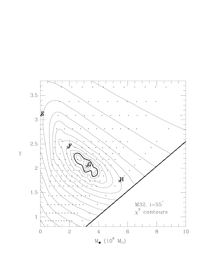
Figure 2: Contours of constant $\chi^{2}$ that measure the goodness-of-fit of axisymmetric models to kinematical data for M32 (van der Marel et al. 1998). The abscissa is the mass of a central point representing a nuclear black hole; the ordinate is the mass-to-light ratio of the stars. These two parameters together specify the potential $\Phi(R,z)$. Each dot represents a single model constructed by varying the orbital population so as to best reproduce the observations in the specified potential. The plateau of nearly-constant $\chi^{2}$ corresponds to models in which changes in $\Phi$ can be compensated for by changes in the orbital population, leaving the goodness-of-fit essentially unchanged.

Orbit-based algorithms like Fillmore & Levison’s have now been written by a number of groups (Gebhardt et al. (1998); van der Marel et al. (1998); Valluri (1998)). In spite of Fillmore & Levison’s discouraging conclusions about the degeneracy of solutions, the most common application of these algorithms is to potential estimation, i.e. inferring the form of $\Phi(R,z)$ based on observed rotation curves and velocity dispersion profiles. A standard approach is to represent $\Phi$ in terms of a small set of parameters; for every choice of parameters, the $f$ is found that best reproduces the kinematical data, and the optimum $\Phi$ is defined in terms of the parameters for which the derived $f$ provides the best overall fit. For instance, $\Phi$ may be written

$$\Phi(R,z)=\left({M\over L}\right)\Phi_{L}(R,z)-{GM_{h}\over r}$$ (31)

where $M/L$ is the mass-to-light ratio of the stars, $\Phi_{L}$ is the “potential” corresponding to the observed luminosity distribution, and $M_{h}$ is the mass of a central black hole. An example is given in Figure 2 which shows $\chi^{2}$ contours in $(M_{h},M/L)$-space derived from ground-based and HST data for M32 (van der Marel et al. (1998)). The expected degeneracy appears as a plateau of nearly constant $\chi^{2}$; this plateau reflects the freedom to adjust a three-integral $f$ in response to changes in $\Phi$ such that the goodness-of-fit to the data remains precisely unchanged. When the potential is represented by just two parameters, this non-uniqueness appears as a ridge line in parameter space, since the virial theorem implies a unique relation between the two parameters that define the potential (Merritt (1994)). Imperfections in the data or the modelling algorithm broaden this ridge line into a plateau, often with spurious local minima. The extreme degeneracy of models derived from such data means that is usually impossible to learn much about the potential that could not have been inferred from the virial theorem alone.

3.4 The Axisymmetric Inverse Problem

Modelling of elliptical galaxies has evolved in a very different way from modelling of disk galaxies, where it was recognized early on that most of the information about the mass distribution is contained in the velocities, not in the light. By contrast, most attempts at elliptical galaxy modelling have used the luminosity as a guide to the mass, with the velocities serving only to normalize the mass-to-light ratio. One could imagine doing much better, going from the observed velocities to a map of the gravitational potential. The difficulties in such an “inverse problem” approach are considerable, however. The desired quantity, $\Phi$, appears implicitly as a non-linear argument of $f$, which itself is unknown and must be determined from the data. There exist few uniqueness proofs that would even justify searching for an optimal solution, much less algorithms capable of finding those solutions.

A notable attempt was made by Merrifield (1991), who asked whether it was possible to infer a dependence of $f$ on a third integral in a model-independent way. Merrifield pointed out that the velocity dispersions along either the major or minor axes of an edge-on, two-integral axisymmetric galaxy could be independently used to evaluate the kinetic energy term in the virial theorem. A discrepancy between the two estimates might be taken as evidence for a dependence of $f$ on a third integral. Merrifield’s test may be seen as a consequence of the fact that $f(E,L_{z})$ is uniquely determined in an axisymmetric galaxy with known $\Phi$ and $\nu$. However, as Merrifield emphasized, a spatially varying $M/L$ could mimic the effects of a dependence of $f$ on a third integral.

An algorithm for simultaneously recovering $f(E,L_{z})$ and $\Phi(R,z)$ in an edge-on galaxy, without any restrictions on the relative distribution of mass and light, was presented by Merritt (1996). The technique requires complete information about the rotational velocity and line-of-sight velocity dispersion over the image of the galaxy. One can then deproject the data to find unique expressions for $\sigma(R,z)$, $\sigma_{\phi}(R,z)$ and $\overline{v_{\phi}}(R,z)$. Once these functions are known, the potential follows immediately from either of the Jeans equations (25, 26); $f_{+}(E,L_{z})$ is also uniquely determined, as described above. The odd part of $f$ is obtained from the deprojected $\overline{v_{\phi}}(R,z)$. This work highlights the impossibility of ruling out two-integral $f$’s for axisymmetric galaxies based on observed moments of the velocity distribution, since the potential can always be adjusted in such a way as to reproduce the data without forcing $f$ to depend on a third integral.

The algorithm just described may be seen as the generalization to edge-on axisymmetric systems of algorithms that infer $f(E)$ and $\Phi(r)$ in spherical galaxies from the velocity dispersion profile (e. g. Gebhardt & Fischer (1995)). The spherical inverse problem is highly degenerate if $f$ is allowed to depend on $L^{2}$ as well as $E$ (e.g. Dejonghe & Merritt (1992)), and one expects a similar degeneracy in the axisymmetric inverse problem if $f$ is allowed to depend on $I_{3}$. Thus the situation is even more discouraging than envisioned by Fillmore & Levison (1989), who assumed that the data were restricted to the major or minor axes: even knowledge of the velocity moments over the full image of a galaxy is likely to be consistent with a large number of $(f,\Phi)$ pairs. Distinguishing between these possible solutions clearly requires additional information, and one possible source is line-of-sight velocity distributions (LOSVD’s), which are now routinely measured with high precision (Capaccioli & Longo (1994)). In the spherical geometry, LOSVD’s have been shown to be effective at distinguishing between different $f(E,L^{2})-\Phi(R,z)$ pairs that reproduce the velocity dispersion data equally well (Merritt & Saha (1993); Gerhard (1993); Merritt (1993)). A second possible source of information is proper motions, which in the spherical geometry allow one to infer the variation of velocity anisotropy with radius (Leonard & Merritt (1989)); however most elliptical galaxies are too distant for stellar proper motions to be easily measured. A third candidate is X-ray gas, from which the potential can in principle be mapped using the equation of hydrostatic equilibrium (Sarazin (1988)).

All of the techniques described above begin from the assumption that the luminosity distribution $\nu(R,z)$ is known. Rybicki (1986) pointed out the remarkable fact that $\nu$ is uniquely constrained by the observed surface brightness distribution of an axisymmetric galaxy only if the galaxy is seen edge-on, or if some other restrictive condition applies, e.g. if the isodensity contours are assumed to be coaxial ellipsoids with known axis ratios. Gerhard & Binney (1996) constructed axisymmetric density components that are invisible when viewed in projection and showed how the range of possible $\nu$’s increases as the inclination varies from edge-on to face-on. Kochanek & Rybicki (1996) developed methods to produce families of density components with arbitrary equatorial density distributions; such components typically look like disks. Romanowsky & Kochanek (1997) explored how uncertainties in deprojected $\nu$’s affect computed values of the kinematical quantities in two-integral models with constant mass-to-light ratios. They found that large variations could be produced in the meridional plane velocities but that the projected profiles were generally much less affected.

These studies suggest that the dynamical inverse problem for axisymmetric galaxies is unlikely to have a unique solution except under fairly restrictive conditions. This fact is useful to keep in mind when evaluating axisymmetric modelling studies, in which conclusions about the preferred dynamical state of a galaxy are usually affected to some degree by restrictions placed on the models for reasons of computational convenience only.

4 TRIAXIALITY

Motion in triaxial potentials differs in three important ways from motion in axisymmetric potentials. First, the lack of rotational symmetry means that no component of an orbit’s angular momentum is conserved. While tube orbits that circulate about the symmetry axes still exist in triaxial potentials, other orbits are able to reverse their sense of rotation and approach arbitrarily closely to the center. The box orbits of Stäckel potentials are prototypical examples. Second, triaxial potentials are 3 DOF systems, and the objects that lend phase space its structure are the resonant tori that satisfy a condition between the three fundamental frequencies of the form $l\omega_{1}+m\omega_{2}+n\omega_{3}=0$. Unlike the case of 2 DOF systems, where a resonance between two fundamental frequencies implies commensurability and hence closure, the resonant trajectories in 3 DOF systems are not generically closed; instead, they densely fill a thin, two-dimensional surface. Third, much of the phase space in realistic triaxial potentials is chaotic, particularly in models where the gravitational force rises rapidly toward the center.

The original motivation for studying triaxial models came from the observed slow rotation of elliptical galaxies (Bertola & Capaccioli (1975); Illingworth (1977)), which effectively ruled out “isotropic oblate rotator” models. The low rotation could have been explained without invoking triaxiality, since any axisymmetric model can be made nonrotating by requiring equal numbers of stars to circulate in the two senses about the symmetry axis. But Binney (1978) argued that it was more natural to grant the existence of a global third integral, hence to assume that the flattening was due in part to anisotropy in the meridional plane. Binney argued further that two non-classical integrals were no less natural than one, and therefore that one might be able to build galaxies without rotational symmetry whose elongated shapes were supported primarily by the extra integrals. This suggestion was confirmed by Schwarzschild (1979, 1982) who showed that most of the orbits in triaxial potentials with large smooth cores do respect three integrals and that self-consistent triaxial models could be constructed by superposition of such orbits. Subsequent support for the triaxial hypothesis came from $N$-body simulations of collapse in which the final configurations were often found to be non-axisymmetric (Wilkinson & James (1982); van Albada (1982)).

The case for triaxiality is perhaps less compelling now than it was ten or fifteen years ago. $N$-body simulations of galaxy formation that include a dissipative component often reveal an evolution to axisymmetry in the stars once the gas has begun to collect in the center (Udry (1993); Dubinski (1994); Barnes & Hernquist (1996)). A central point mass, representing a nuclear black hole, has a similar effect (Norman, May & van Albada (1985); Merritt & Quinlan (1998)). A plausible explanation for the evolution toward axisymmetry in these simulations is stochasticity of the box orbits resulting from the deepened central potential. Similar conclusions have been drawn from self-consistency studies of triaxial models with realistic, centrally-concentrated density profiles: the shortage of regular box orbits is often found to preclude a stationary triaxial solution (Schwarzschild (1993); Merritt & Fridman (1996); Merritt (1997)). Observational studies of minor-axis rotation suggest that few if any elliptical galaxies are strongly triaxial (Franx, Illingworth & de Zeeuw (1991)), and detailed modelling of a handful of nearby ellipticals, as discussed above, reveals that their kinematics can often be very well reproduced by assuming axisymmetry. The assumption that an oblate galaxy with counter-rotating stars would be unphysical has also been weakened by the discovery of a handful of such systems (Rubin, Graham & Kenney (1992); Merrifield & Kuijken (1994)).

The phenomenon of triaxiality nevertheless remains a topic of vigorous study, for a number of reasons. At least some elliptical galaxies and bulges exhibit clear kinematical signatures of non-axisymmetry (s.g. Schechter & Gunn (1979); Franx, Illingworth & Heckman (1989)), and the observed distribution of Hubble types is likewise inconsistent with the assumption that all ellipticals are precisely axisymmetric (Tremblay & Merritt (1995), 1996; Ryden (1996)). Departures from axisymmetry (possibly transient) are widely argued to be necessary for the rapid growth of nuclear black holes during the quasar epoch (Shlosman, Begelman & Frank (1990)), for the fueling of starburst galaxies (Sanders & Mirabel (1996)), and for the large radio luminosities of some ellipticals (Bicknell et al. (1997)). These arguments suggest that most elliptical galaxies or bulges may have been triaxial at an earlier epoch, and perhaps that triaxiality is a recurrent phenomenon induced by mergers or other interactions.

Almost all of the work reviewed below deals with nonintegrable triaxial models. Integrable triaxial potentials do exist – the Perfect Ellipsoid is an example – but the integrable models always have features, like large, constant-density cores, that make them poor representations of real elliptical galaxies. More crucially, integrable potentials are “non-generic” in the sense that their phase space lacks many of the features that are universally present in non-integrable potentials. For instance, the box orbits in realistic triaxial potentials are strongly influenced by resonances between the three degrees of freedom, while in integrable potentials these resonances (although present) have no effect and all the box orbits belong to a single family. Integrable triaxial models are reviewed by de Zeeuw (1988) and Hunter (1995).

The standard convention is adopted here in which the long and short axes of a triaxial figure are identified with the $x$ and $z$ axes respectively.

4.1 The Structure of Phase Space

The motion in smooth triaxial potentials has many features in common with more general dynamical systems. Some relevant results from Hamiltonian dynamics are reviewed here before discussing their application to triaxial potentials.

Motion in non-integrable potentials is strongly influenced by resonances between the fundamental frequencies. A resonant torus is one for which the frequencies $\omega_{i}$ satisfy a relation ${\bf n\cdot\omega}=0$ with ${\bf n}=(l,m,n)$ an integer vector. Resonances are dense in the phase space of an integrable Hamiltonian, in the sense that every torus lies near to a torus satisfying ${\bf n\cdot\omega}=0$ for some (perhaps very large) integer vector $\bf n$. However, most tori are very non-resonant in the sense that ${\bf n}\cdot\omega$ is large compared with $|{\bf n}|^{-(N+1)}$, with $N$ the number of degrees of freedom. As one gradually perturbs a Hamiltonian away from integrable form, the KAM theorem guarantees that the very non-resonant tori will retain their topology, i.e. that the motion in their vicinity will remain quasiperiodic and confined to (slightly deformed) invariant tori. Resonant tori, on the other hand, can be strongly affected by even a small perturbation.

In a 2 DOF system, motion on a resonant torus is closed, since the resonance condition implies that the two frequencies are expressible as a ratio of integers, $\omega_{1}/\omega_{2}=|m/l|$. In three dimensions, a single relation ${\bf n\cdot\omega}=0$ between the three frequencies does not imply closure; instead, the trajectory is confined to a two-dimensional submanifold of its 3-torus. The orbit in configuration space lies on a thin sheet. (In the special case that one of the elements of ${\bf n}$ is zero, two of the frequencies will be commensurate.) For certain tori, two independent resonance conditions ${\bf n\cdot\omega}=0$ will apply; in this case, the fundamental frequencies can be written $\omega_{i}=n_{i}\omega_{0}$, i.e. there is commensurability for each frequency pair and the orbit is closed.

On a resonant torus in an integrable Hamiltonian, every trajectory satisfies the resonance conditions (of number $K\leq N-1$) regardless of its phase. Among this infinite set of resonant trajectories, only a finite number persist under perturbation of the Hamiltonian, as resonant tori of dimension $N-K$. The character of these remaining tori alternates from stable to unstable as one varies the phase around the original torus. Motion in the vicinity of a stable resonant torus is regular and characterized by $N$ fundamental frequencies. Motion in the vicinity of an unstable torus is generically stochastic, even for small perturbations of the Hamiltonian. Furthermore, in the neighborhood of a stable resonant torus, higher-order resonances occur which lead to secondary regions of regular and stochastic motion, etc., down to finer and finer scales.

In a weakly perturbed Hamiltonian, the stochastic regions tend to be isolated and the associated orbits are often found to mimic regular orbits for many oscillations. As the perturbation increases, the stochastic regions typically grow at the expense of the invariant tori. Eventually, stochastic regions associated with different unstable resonances overlap, producing large regions of phase space where the motion is interconnected. One often observes a sudden transition to large-scale or “global” stochasticity as some perturbation parameter is varied. In a globally stochastic part of phase space, different orbits are effectively indistinguishable and wander in a few oscillations over the entire connected region. Such orbits rapidly visit the entire configuration space region within the equipotential surface, giving them a time-averaged shape that is approximately spherical.

The way in which resonances affect the phase space structure of nonrotating triaxial potentials has recently been clarified by a number of studies (Carpintero & Aguilar (1998); Papaphilippou & Laskar (1998); Valluri & Merritt (1998)) that used trajectory-following algorithms to extract the fundamental frequencies and to identify stochastic orbits. The discussion that follows is based on this work and on the earlier studies of Levison & Richstone (1987), Schwarzschild (1993) and Merritt & Fridman (1996).

At a fixed energy, the phase space of a triaxial galaxy is five-dimensional. One expects most of the regular orbits to be recoverable by varying the initial conditions over a space of lower dimensionality; for instance, in an integrable potential, all the orbits at a given energy can be specified via the 2D set of actions. Levison & Richstone (1987) advocated a 4D initial condition space consisting of coordinates $(x_{0},z_{0},y_{0}=0)$ and velocities $(\dot{x}_{0},\dot{z}_{0})$, with $\dot{y}_{0}$ determined by the energy. Schwarzschild (1993) argued that most orbits could be recovered from just two, 2D initial condition spaces. His first space consisted of initial conditions with zero velocity on one octant of the equipotential surface; these initial conditions generate box orbits in Stäckel potentials. The second space consisted of initial conditions in the $(x,z)$ plane with $\dot{x}_{0}=\dot{z}_{0}=0$ and $\dot{y}_{0}$ determined by the energy. This space generates the four families of tube orbits in Stäckel potentials. Papaphilippou & Laskar (1998) suggested that boxlike orbits could be generated more simply by setting all coordinates to zero and varying the two velocity components parallel to a principal plane. This choice for box-orbit initial condition space is not precisely equivalent to Schwarzschild’s; it excludes resonant orbits (e.g. the banana) that avoid the center, while Schwarzschild’s excludes orbits (e.g. the anti-banana) that have no stationary point.

Figure 3a illustrates stationary (box-orbit) initial condition space at one energy in a triaxial Dehnen model with $c/a=0.5$, $b/a=0.79$ and $\gamma=0.5$, a “weak cusp.” The figure was constructed from $\sim 10^{4}$ orbits with starting points lying on the equipotential surface; the greyscale was adjusted in proportion to the logarithm of the stochasticity, measured via the rate of diffusion in frequency space. Initial conditions associated with regular orbits are white. Figure 3b shows the frequency map defined by the same orbits, i.e. the ratios $\omega_{x}/\omega_{z}$ and $\omega_{y}/\omega_{z}$ between the fundamental frequencies associated with motion along the three coordinate axes. The most important resonances, $l\omega_{x}+m\omega_{y}+n\omega_{z}=0$, are indicated by lines in the frequency map and by their integer components $(l,m,n)$ in Figure 3a. Intersections of these lines correspond to closed orbits, $\omega_{i}=n_{i}\omega_{0}$. In order to keep the frequency map relatively simple, all orbits associated with a stable resonance have been plotted precisely on the resonance line; the third fundamental frequency (associated with slow rotation around the resonance) has been ignored. Unstable resonances appear as gaps in the frequency map, since the associated orbits do not have well-defined frequencies.

Figure 3: Box-orbit phase space at roughly the half-mass energy in a triaxial Dehnen model with cusp slope $\gamma=0.5$ (Valluri & Merritt 1998). (a) Initial condition space: one octant of the equipotential surface has been projected onto a plane. Each orbit begins on this surface with zero velocity. The top, left and right corners correspond to the $z$ (short), $x$ (long) and $y$ (intermediate) axes. The grey scale is proportional to the logarithm of the diffusion rate of orbits in frequency space; initial conditions corresponding to regular orbits are white. The regions labelled “1” and “2” are starting points associated with the $5:6:8$ and $7:9:10$ periodic orbits, respectively. Other regions are labelled with the integers $(l,m,n)$ that define resonance zones. (b) Frequency map: the fundamental frequencies are plotted as ratios $\omega_{x}/\omega_{z}$ and $\omega_{y}/\omega_{z}$ for each of the orbits in (a). The most important resonances are labelled. Stable resonances produce solid lines; gaps correspond to unstable (chaotic) resonances.

Following the discussion above, one expects the regular orbits to come in three families corresponding to the number $K=(0,1,2)$ of independent resonance conditions that define their associated phase space regions. The three families are in fact apparent in Figure 3. First are the regular orbits that lie in the regions between the resonance zones, $K=0$. Orbits in these regions are regular for the same reason that box orbits in a Stäckel potential are regular, i.e. because the region of phase space in which they are located is locally integrable. In configuration space, these orbits densely fill a three-dimensional region centered on the orgin. A second set of regular orbits lie in zones associated with a single resonance, $K=1$; examples are the $(2,1,-2)$, $(3,-1,-1)$ and $(4,-2,-1)$ resonance zones. The stable resonant orbits that define these regions are “thin boxes” that fill a sheet in configuration space (Figure 4); the regular orbits around them have a small but finite thickness. The planar $x-z$ banana $(2,0,-1)$ and fish $(3,0,-2)$, and the $x-y$ pretzel $(4,-3,0)$, also generate families of thin orbits. The third set of regular orbits, the “boxlets,” surround periodic orbits that lie at the intersection of two resonances, $K=2$. Two such regions are apparent in Figure 3a, associated with the $5:6:8$ and $7:9:10$ periodic orbits (marked 1 and 2).

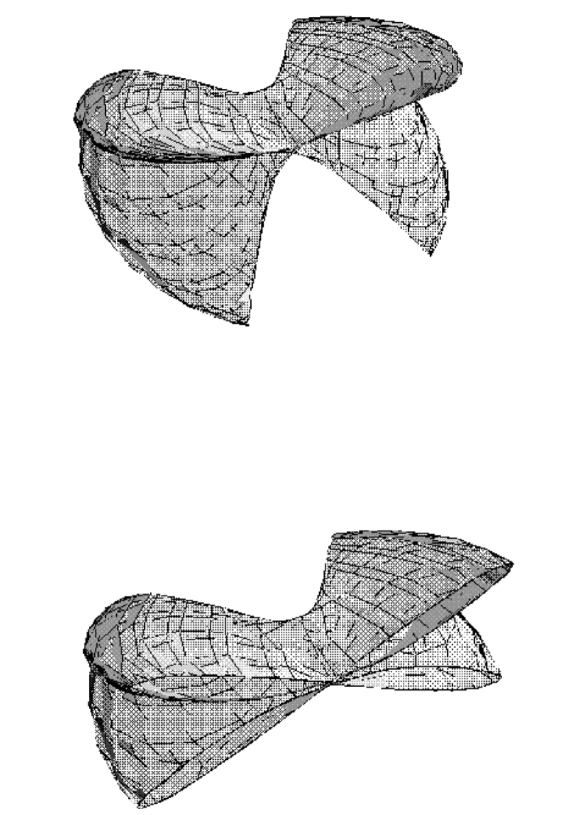
Figure 4: A thin box orbit associated with the $(2,1,-2)$ resonance in Figure 3. The lower view is a cutaway showing that the orbit is confined to a membrane.

Close inspection of Figure 3a suggests that even the “integrable” ($K=0$) regions are threaded with high-order resonances and their associated chaotic zones. One expects to find such structure since resonant tori are dense in the phase space of the unperturbed Hamiltonian. However the stochasticity associated with the high-order resonances is very weak and for practical purposes the orbits in these regions are regular throughout.

All of the box orbits in a Stäckel potential belong to a single family with smoothly varying actions. While resonances like those shown in Figure 3 are present in Stäckel potentials, their effect on the motion is limited to the resonant tori themselves. By contrast, in the phase space of tube orbits, even Stäckel potentials contain (up to) three important resonances at each energy corresponding to the three families of thin tube orbits. These primary resonances persist in nonintegrable potentials and generate families of regular tube orbits similar to those in Stäckel potentials. The transition zones between the various tube orbit families, which are occupied by unstable orbits in a Stäckel potential, are now stochastic, although the stochastic zones are typically narrow. Valluri & Merritt (1998) illustrated the time evolution of a stochastic tube orbit.

The structure in Figure 3 is characteristic of mildly non-integrable triaxial potentials. As the perturbation of the potential away from integrability increases – due to an increasing central density, for instance – the parts of phase space corresponding to tube orbits are only moderately affected. However the boxlike orbits are sensitively dependent on the form of the potential near the center. Papaphilippou & Laskar (1998) studied ensembles of orbits in the logarithmic triaxial potential at fixed energy; they took as their perturbation parameter the axis ratios of the model. At extreme elongations, high-order resonances became important in box-orbit phase space; for instance, in a triaxial model with $c/a=0.18$, significant stochastic regions associated with the $(3,-1,0)$ and $(6,-1,-1)$ resonances were found. Valluri & Merritt (1998) varied the cusp slope $\gamma$ and the mass of a central black hole in a family of triaxial Dehnen models. They found that the relative contributions from the three types of regular orbit (satisfying 0, 1, or 2 resonance conditions) in box-orbit phase space shifted as the perturbation increased, from $K=0$ (box orbits) at small perturbations, to $K=1$ (thin boxes) at moderate perturbations, to $K=2$ (boxlets) at large perturbations.

4.2 Periodic Orbits

As discussed above, the objects that give phase space its structure in 3 DOF systems are the resonant tori which satisfy a condition $l\omega_{1}+m\omega_{2}+n\omega_{3}=0$ between the three fundamental frequencies. The corresponding orbits are thin tubes or thin boxes. However most studies of the motion in triaxial potentials have focussed on the principal planes, in which resonances (i.e. $l\omega_{1}+m\omega_{2}=0$) are equivalent to closed orbits. Figure 3a suggests that most of the regular orbits in a triaxial potential are associated with thin orbits rather than with closed orbits. The closed orbits are nevertheless worth studying for a number of reasons. Gas streamlines must be non-self-intersecting, which restricts the motion of gas clouds to closed orbits like the $1:1$ loops. Elongated boxlets like the bananas have shapes that make them very useful for reproducing a barlike mass distribution, and one expects such orbits to be heavily populated in self-consistent models. The fraction of regular orbits associated with closed orbits (as opposed to thin orbits) also tends to increase as the phase space becomes more and more chaotic, as discussed below.

4.2.1 Nonrotating Potentials

Periodic orbits in the principal planes of triaxial models often first appear as bifurcations from the axial orbits. Figure 5 is a representative bifurcation diagram for axial orbits in nonrotating triaxial models with finite central forces, based on the studies of Heiligman & Schwarzschild (1979), Goodman & Schwarzschild (1981), Magnenat (1982a), Binney (1982a), Merritt & de Zeeuw (1983), Miralda-Escudé & Schwarzschild (1989), Pfenniger & de Zeeuw (1989), Lees & Schwarzschild (1992), Papaphilippou & Laskar (1996, 1998), and Fridman & Merritt (1997). When the central force is strongly divergent, as would be the case in a galaxy with a central black hole, the axial orbits are unstable at all energies but many of the other periodic orbits in Figure 5 still exist.

Figure 5: Representative bifurcation diagram for planar periodic orbits in non-axisymmetric potentials with finite central forces. The three rows show bifurcations from the $x$ (long), $y$ (intermediate) and $z$ (short) axes. The left column (S) shows bifurcations in the plane containing the shorter of the two remaining axes, while the right column (L) shows bifurcations in the plane containing the longer axis. Solid lines correspond to stable orbits and dotted lines to unstable orbits, where stability is defined with respect to motion in the appropriate plane.

At low energies in a harmonic core, all three axial orbits are stable. The axial orbits typically change their stability properties at the $n:1$ bifurcations where the frequency of oscillation equals $1/n$ times the frequency of a transverse perturbation. This typically first occurs first along the $y$ (intermediate) axis when the frequency of $y$ oscillations falls to the frequency of an $x$ perturbation, producing a $1:1$ bifurcation. The $y$-axis orbit becomes unstable and a closed $1:1$ loop orbit appears in the $x-y$ plane. The $x-y$ loop is initially elongated in the direction of the $y$ axis but becomes rapidly rounder with increasing energy. Similar $1:1$ bifurcations occur at slightly higher energies from the $z$ axis: first in the $y-z$ plane, then in the $x-z$ plane, producing two more planar loop orbit families. The $x-z$ loop is typically unstable to vertical perturbations; the other two loops are generally stable and generate the long- and short-axis tube orbit families.

The $x$-axis orbit does not experience a $1:1$ bifurcation since its frequency is always less than that of perturbations along either of the two shorter axes. However at sufficiently high energies, the $x$ oscillation frequency falls to $1/2$ the frequency of a $z$ perturbation and the $2:1$ $x-z$ banana orbit appears (Figure 6). At still higher energies, a second $2:1$ bifurcation produces the $x-y$ banana; following this bifurcation, the $x$-axis orbit is typically unstable in both directions. This second bifurcation occurs most readily in nearly prolate models where the $y$ and $z$ axes are nearly equal in length. The energy of the first, $x-z$ bifurcation is a strong function of the degree of central concentration of the model, as measured for instance by the cusp-slope parameter $\gamma$ in Dehnen’s model. For $\gamma\mathrel{\mathchoice{\lower 3.6pt\vbox{\halign{$\mathsurround=0pt\displaystyle\hfil#\hfil$\cr>\crcr\sim\crcr}}}{\lower 3.6pt\vbox{\halign{$\mathsurround=0pt\textstyle\hfil#\hfil$\cr>\crcr\sim\crcr}}}{\lower 3.6pt\vbox{\halign{$\mathsurround=0pt\scriptstyle\hfil#\hfil$\cr>\crcr\sim\crcr}}}{\lower 3.6pt\vbox{\halign{$\mathsurround=0pt\scriptscriptstyle\hfil#\hfil$\cr>\crcr\sim\crcr}}}}1$, the $x$-axis orbit is unstable at most energies in all but the roundest triaxial models.

Figure 6: Resonant box orbits in a principal plane of a triaxial potential. Left: centrophobic boxlets; these are typically stable. Right: centrophilic boxlets; these are typically unstable.

In highly elongated models, $c/a\mathrel{\mathchoice{\lower 3.6pt\vbox{\halign{$\mathsurround=0pt\displaystyle\hfil#\hfil$\cr<\crcr\sim\crcr}}}{\lower 3.6pt\vbox{\halign{$\mathsurround=0pt\textstyle\hfil#\hfil$\cr<\crcr\sim\crcr}}}{\lower 3.6pt\vbox{\halign{$\mathsurround=0pt\scriptstyle\hfil#\hfil$\cr<\crcr\sim\crcr}}}{\lower 3.6pt\vbox{\halign{$\mathsurround=0pt\scriptscriptstyle\hfil#\hfil$\cr<\crcr\sim\crcr}}}}0.45$, the $x$ axis orbit can return to stability at the bifurcation of the “antibanana” orbit, a $2:1$ resonant orbit that passes through the center (Figure 6). Miralda-Escudé & Schwarzschild (1989) call such orbits “centrophilic;” resonant orbits that avoid the center, like the $x-z$ banana, are “centrophobic.” In nearly oblate models, this return to stability in the $x-z$ plane causes the $x$-axis orbit to become stable in both directions. The $x$-axis orbit can become unstable once more at still higher energies when $c/a$ is sufficiently small, through the appearance of a $3:1$ resonance in the direction of the $z$ axis.

Both the $y$- and $z$-axis orbits are unstable at all energies above the $1:1$ bifurcations. The $y$-axis orbit can become unstable in both directions following the $2:1$ bifurcation that produces the $y-z$ banana. In highly elongated models, the $y$-axis orbit returns briefly to stability in the $z$-direction through the appearance of the $y-z$ anti-banana.

Additional bifurcations of the form $n:m$, with both $n$ and $m$ greater than one, can occur from the axial orbits. These bifurcations typically do not affect the stability of the axial orbits but they are nevertheless important because they generate additional families of periodic orbits. The name “boxlet” was coined by Miralda-Escudé & Schwarzschild (1989) for these orbits (Figure 6). The $3:2$ boxlets are “fish,” the $4:3$ boxlets are “pretzels,” etc. Only the fish orbits have been extensively studied; they first appear as $3:2$ bifurcations from the $x$-axis orbit ($x-z$ and $x-y$ fish) or the $y$-axis orbit ($y-z$ fish), typically at energies below the banana bifurcation. The $x-y$ fish is only important in highly prolate models.

The boxlets can themselves become unstable, either to perturbations in the plane of the orbit or to vertical perturbations. The $x-z$ banana exists and is stable over a wide range of model parameters; it becomes unstable only in nearly prolate models, through a vertical $2:1$ bifurcation. The $x-y$ and $y-z$ bananas are usually vertically unstable; the $x-y$ banana returns to stability only in highly elongated, nearly prolate models. In nearly oblate models, the $x-z$ fish first becomes unstable to perturbations in the orbital plane, while for strongly triaxial and prolate models instability first appears in the vertical ($y$) direction. The $x-y$ fish is only important in strongly prolate models; in strongly triaxial or oblate models, it either does not exist, or is generally unstable to vertical perturbations. The $y-z$ fish is almost always vertically unstable.

As the central concentration of a triaxial model increases, the axial orbits become unstable over a progressively wider range of energies. In models with steep central cusps or central black holes, the axial orbits are unstable at all energies and the (centrophobic) boxlets may extend all the way to the center. Little systematic work has been done on the properties of boxlets in such models. Miralda-Escudé & Schwarzschild (1989) investigated the orbit structure in the principal planes of two triaxial models with $\Phi=\log\left(R_{c}^{2}+m^{2}\right)$ as $R_{c}$ was varied; for $R_{c}=0$, their models have an $r^{-2}$ central density cusp. Miralda-Escudé & Schwarzschild found that the lowest-order boxlets continued to exist, typically with no change in their stability properties, as $R_{c}$ was reduced to zero. The centrophobic boxlets were also found to be not strongly affected by the addition of a central point mass. Pfenniger & de Zeeuw (1989) investigated the banana boxlets in a second family of models with $\gamma=2$ cusps. They found that the bananas became strongly bent for model axis ratios $c/a\mathrel{\mathchoice{\lower 3.6pt\vbox{\halign{$\mathsurround=0pt\displaystyle\hfil#\hfil$\cr<\crcr\sim\crcr}}}{\lower 3.6pt\vbox{\halign{$\mathsurround=0pt\textstyle\hfil#\hfil$\cr<\crcr\sim\crcr}}}{\lower 3.6pt\vbox{\halign{$\mathsurround=0pt\scriptstyle\hfil#\hfil$\cr<\crcr\sim\crcr}}}{\lower 3.6pt\vbox{\halign{$\mathsurround=0pt\scriptscriptstyle\hfil#\hfil$\cr<\crcr\sim\crcr}}}}0.65$, making them less useful for reconstructing the model shape. In their survey of orbits in two triaxial models with Dehnen’s density law, Merritt & Fridman (1996) found that the $x-z$ fish was vertically unstable at most energies for $\gamma=1$ and at all energies for $\gamma=2$. Only the $x-z$ fish, of all the planar boxlet families, remained stable over an appreciable energy range in the two models investigated by them. A number of higher-order resonances outside of the principal planes were also found to be important, including the $4:5:7$, $5:6:8$ and $6:7:9$ boxlets.

4.2.2 Rotating Models

A great deal of work has been done on periodic orbits in models of barred galaxies (Contopoulos & Grosbøl (1989); Sellwood & Wilkinson (1993)). Most of this work has been restricted to motion in the equatorial plane; furthermore, models of barred galaxies typically have low central concentrations, mild departures from axisymmetry (“weak bars”), and rapid rotation, making them poor representations of elliptical galaxies. The smaller number of studies of periodic orbits in rotating elliptical galaxy models have focussed on two low-order resonant families: the $1:1$ orbits that bifurcate from the axial orbits, giving rise to the tubes; and the $1:2$ banana orbits.

An early study of the closed orbits in Schwarzschild’s (1979) triaxial model (Merritt (1979)) revealed that the $1:1$ orbits circling the long axis continue to exist when the figure rotates, but are tipped by the Coriolis force out of the $y-z$ plane. The tip angle increases with energy and the family terminates when it mergers with the retrograde closed orbits in the equatorial plane. Heisler, Merritt & Schwarzschild (1982) called these tipped orbits “anomalous” and noted the existence of a second, unstable family of anomalous orbits circling the intermediate axis. A large number of additional studies have traced the existence and stability of these orbits in a variety of rotating triaxial potentials (Binney (1981); Tohline & Durisen (1982); Magnenat 1982a , b; de Zeeuw & Merritt (1983); Durisen et al. (1983); Merritt & de Zeeuw (1983); Mulder (1983); Mulder & Hooimeyer (1984); Martinet & de Zeeuw (1988); Cleary (1989); Patsis & Zachilas (1990); Hasan, Pfenniger & Norman (1993)). One motivation for this work has been the expectation that gas or dust falling into a rotating triaxial galaxy might dissipatively settle onto the anomalous orbits before finding its way into the center (Tohline & Durisen (1982); van Albada, Kotanyi & Schwarzschild (1982)).

The existence of the anomalous orbits is tied to the vertical instability of the orbits in the equatorial plane. There are four major families of planar orbits: two of these (the “$x_{1}$” and “$x_{4}$” families in Contopoulos’s convention), both prograde, remain close to the $x$ and $y$ axes respectively; the other two ($x_{2}$ and $x_{3}$) are prograde and retrograde counterparts of the $1:1$ orbit that bifurcates from the $y$ axis in nonrotating models. One of these – either the retrograde orbit, if figure rotation is about the short axis, or the prograde orbit, if rotation is about the long axis – is unstable to perturbations out of the plane of rotation over a wide radial range. In either case, a family of anomalous orbits exists that is inclined to the plane of rotation; the family has two branches that are tipped in opposite directions with respect to the equatorial plane but which circle the short axis in the same sense. The anomalous orbits first appear at low energies as $1:1$ bifurcations of the $z-$ axis orbit. In models without cores, the $z$-axis orbit may be unstable at all energies and the anomalous orbits extend into the center. In models with sufficiently high rotation, on the other hand, the anomalous orbits can bifurcate twice from the family in the plane, never reaching the $z$-axis. The unstable anomalous orbits that circle the intermediate axis first appear at the bifurcation of the $1:1$ orbit in the $x-z$ plane.

Miller & Smith (1979) investigated the motion of particles in a 3D, rotating $N$-body bar. They found that nearly half of the orbits could be described as respecting a $2:1$ resonance between the $x$ and $z$ motions. Pfenniger & Friedli (1991) likewise found a large population of $2:1$ orbits in their rotating $N$-body models. This family of orbits, which reduces to the $x-z$ bananas in the case of zero figure rotation, has been studied by a number of other authors including Mulder & Hooimeyer (1984), Cleary (1989), Martinet & Udry (1990), Patsis & Zachilas (1990), Udry (1991), and Hasan, Pfenniger & Norman (1993). The family bifurcates from the prograde $x_{1}$ family at low energies and so retains the $x-y$ commensurability of that orbit – either $1:1$ (low energies) or $3:1$ (high energies). The radial range over which it exists decreases with increasing rotation of the figure. At large energies, the $x_{1}$ orbit returns to vertical stability through bifurcation of the $x-z$ anti-banana. At even greater energies, both banana families may merge again with the $x_{1}$ orbits. Udry (1991) traced the existence and stability of the $2:1$ orbits that bifurcate from the $y$ and $z$ axes and from the other $1:1$ families in the equatorial plane. None of these families is likely to be as important as the $x-z$ bananas in self-consistent models.

4.3 Stochasticity

4.3.1 Origin

Stochasticity always occurs near an unstable resonant torus. Such tori exist and are dense even in integrable systems, but the motion in their vicinity is (by definition) regular; under perturbation of the potential, however, resonant tori are destroyed and the motion undergoes a qualitative change. The reason for this change is suggested by Figure 7, which shows an orbit that lies close to the short- ($y$-) axis orbit in the potential of a 2D bar. Such an orbit can be represented as the superposition of a rapid radial oscillation and a slow angular rotation, with frequencies $\omega_{r}$ and $\omega_{\theta}$ respectively; $\omega_{\theta}$ tends to zero as the orbit approaches the axial orbit. Resonances between the fast and slow motions satisfy a condition $l\omega_{\theta}-m\omega_{r}=0$. As $\omega_{\theta}$ tends to zero, the separation between neighboring resonances, defined by $l$ and $l+1$, also becomes small, resulting in motion that is extremely complex. In fact one can show that the motion is generically no longer confined to tori; instead the trajectory moves more-or-less randomly through a region of dimensionality $2N-1$, where $N$ is the number of degrees of freedom. Among the properties of the motion in these stochastic regions is exponential divergence of initially close trajectories (Miller (1964); Oseledec (1968)), resulting in extreme sensitivity to small changes in the initial conditions.

Figure 7: An orbit that lies close to the unstable, short- ($y$-) axis orbit in a 2D barred potential. The motion consists of a rapid radial oscillation combined with a slow rotation. Resonances between the fast and slow motions produce a stochastic zone where the motion is exponentially unstable.

An early indication of the importance of stochasticity in triaxial potentials was the discovery that some of the orbits in Schwarzschild’s (1979) triaxial model yielded different occupation numbers when integrated using a different computer (Merritt (1980)), a consequence of the exponential divergence just mentioned. Goodman & Schwarzschild (1981) computed rates of divergence between pairs of box-orbit trajectories at one energy in this potential; they found that about a fourth of the orbits were stochastic. Most of the unstable orbits had their starting points near the $z$ axis, producing a narrow strip of instability in initial condition space; a similar stochastic strip can be seen in Figure 3a. Goodman & Schwarzschild showed that both the $y$ and $z$ axis orbits were linearly unstable at this energy while the $x$ axis orbit was stable. They speculated that the stochasticity was connected with this instability; in particular, they noted that the $z$-axis orbit was strongly unstable to perturbations in both directions, following the bifurcation of the $1:1$ loop orbits in the $y-z$ and $x-z$ planes.

The stochasticity of the motion near the short axis orbit (as opposed to the instability of the axial orbit, a weaker condition) was established by Gerhard (1985) using a method due to Melnikov (1963). Melnikov’s method is based on the qualitative change that occurs in the shape of the phase curve, or “separatrix,” of an unstable 2D orbit in the surface of section when the motion in its vicinity becomes stochastic. In a two-dimensional integrable potential, the separatrix is a smooth curve that intersects itself at the fixed (“homoclinic”) point corresponding to an unstable orbit like the one in Figure 7. Under perturbation, the two branches of the separatrix corresponding to motion toward and away from the fixed point need not join smoothly; instead they can oscillate wildly, producing an infinite set of additional homoclinic points. The stochasticity may be interpreted as a consequence of this complex behavior. Melnikov defined an integral quantity that measures the infinitesimal separation between the two branches of the separatrix that approach and depart from the unstable fixed point. If this distance changes sign as one proceeds around the separatrix, nonintegrability has been rigorously established. Gerhard took as his integrable potential a 2D Stäckel model in which the total density fell off as $r^{-2}$ and the non-axisymmetric component as $r^{-4}$. He showed that certain perturbations, e.g. density terms varying as $\cos(m\phi)$ with $m$ odd, produced a rapid breakdown in the regularity of the motion near the short-axis orbit.

Martinet & Udry (1990) noted that most of the stochasticity in slowly-rotating planar models appeared to be associated with the $x_{3}$ family, which reduces to the unstable short-axis orbit in the limit of zero rotation. They traced the interactions of higher-order resonances in the vicinity of the $x_{3}$ orbit and argued that the development of a large stochastic layer in the surface of section could be attributed to the simultaneous action of these resonances. Martinet & Udry found that the stochastic region associated with this orbit tended to contract as the rate of figure rotation increased.

The $1:1$ bifurcation that first induces instability in the $z$-axis orbit occurs at lower and lower energies as the central concentration of a triaxial model is increased. At the same time, the sensitivity of the axial orbits to small perturbations increases as the central force steepens. These two facts imply a greater role for stochasticity in triaxial models with high central densities. Gerhard & Binney (1985) investigated 2 DOF motion in a bar with a central density cusp, $\rho\sim r^{-\gamma}$, or a central point mass $M_{h}$ representing a supermassive black hole. Using surfaces of section, they found that the fraction of phase space associated with stochastic motion increased with increasing $\gamma$ or $M_{h}$. However, regular boxlike orbits persisted in families associated with low-order resonances like the $2:1$ banana. Miralda-Escudé & Schwarzschild (1989) studied the orbits in a planar logarithmic potential as a function of core radius $R_{c}$. Even for $R_{c}=0$, corresponding to a $\rho\sim r^{-2}$ density cusp, the stochastic regions were found to be confined to narrow filaments in the surface of section between the resonant families. Papaphilippou & Laskar (1996) likewise found only a modest degree of stochasticity in their study of 2D logarithmic potentials with cores. Touma & Tremaine (1997) obtained similar results in the planar logarithmic potential using an approximate mapping technique.

Studies like these of 2 DOF motion tend to underestimate the importance of stochasticity in triaxial potentials, for at least three reasons. Periodic orbits that generate families of regular trajectories in the principal planes are often unstable to perturbations out of the plane; examples are the $x-y$ and $y-z$ bananas discussed above. Second, there are unstable periodic orbits that exist outside of the principal planes; some examples can be seen in Figure 3. Third, much of the stochasticity in 3 DOF systems is associated with resonances between the three degrees of freedom which have no analog in 2 DOF systems.

Techniques like surfaces of section that work well in 2 DOF systems can become cumbersome in three dimensions. An alternative technique for identifying an orbit as stochastic is to compute its Liapunov exponents, the mean exponential rates of divergence of a set of trajectories surrounding it. In a 3 DOF system there are six Liapunov exponents for every trajectory, corresponding to the six dimensions of phase space; the exponents come in pairs of opposite sign, a consequence of the conservation of phase space volume. Of the three independent exponents, one – corresponding to displacements in the direction of the motion – is always zero. The two remaining exponents, $\sigma_{1}$ and $\sigma_{2}$, may be seen as defining the time-averaged divergence rates in two directions orthogonal to the trajectory. For a regular orbit, $\sigma_{1}=\sigma_{2}=0$; for a stochastic orbit, at least one (and typically two) of these exponents is nonzero.

Udry & Pfenniger (1988) computed all six Liapunov exponents for ensembles of orbits in triaxial potentials based on a modified Hubble law, which has a constant-density core and a large-radius density dependence of $r^{-3}$. To this model they added perturbing forces of various kinds, corresponding to central mass concentrations and angular distortions of the density. Udry & Pfenniger presented their results in terms of histograms of Liapunov exponents without distinguishing between different types of orbit or between orbits of different energies. Nevertheless they found that the average degree of stochasticity for a given potential always increased with increasing strength of the perturbation. Schwarzschild (1993) computed the largest Liapunov exponent for the orbits in his scale-free, $\rho\propto r^{-2}$ triaxial models discussed below. He found that most of the boxlike orbits, and a modest but significant fraction of the tube orbits, were stochastic; the $y-z$ instability strip first discussed by Goodman & Schwarzschild (1981) was typically greatly enlarged in the scale-free models. Merritt & Fridman (1996) demonstrated that the boxlike orbits in a triaxial model with a cusp as shallow as $\rho\sim r^{-1}$ were also mostly stochastic, though many of these orbits mimicked regular orbits for tens or hundreds of orbital periods. They noted that much of the stochasticity was generated by resonances not associated with the $z$-axis orbit. Merritt & Valluri (1996) showed that the histogram of Liapunov exponents of box orbits at a given energy tended toward a narrow spike as the integration time increased, consistent with the expectation that the stochastic parts of phase space are interconnected via the Arnold web. They found that both $\sigma_{1}$ and $\sigma_{2}$ were significantly nonzero for all of their orbits, suggesting that no isolating integrals existed aside from the energy.

4.3.2 Transition to Global Stochasticity

The KAM theorem guarantees that motion in the vicinity of a “very nonresonant” torus in an integrable system will remain regular under small perturbations of the potential. Since the majority of tori are very nonresonant – in the sense that rational numbers are rare compared to irrational ones – the KAM theorem says that a small perturbation of an integrable potential will leave most of the trajectories regular. At the same time, the resonant tori are dense in the phase space, and even an infinitesimal perturbation can cause the motion in their vicinity to become chaotic. When the perturbation is small, these chaotic regions are narrow and the motion within them tends to mimic regular motion for many oscillations. As the perturbation is increased, the chaotic zones from different resonant tori become wider and neighboring zones begin to overlap. Eventually one expects to find large regions of interconnected phase space where the motion is fully stochastic (Hénon & Heiles (1964)).

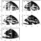
Figure 8: Transition to global stochasticity in stationary (box-orbit) initial condition space (Valluri & Merritt 1998). Each frame shows an octant of the equipotential surface, at roughly the half-mass radius, in a triaxial Dehnen model with $\gamma=0.5$ and with a central point containing a fraction $M_{h}$ of the total mass of the model. The $z$- (short) axis is vertical and the $x$- (long) axis is to the left. The grey scale is proportional to the logarithm of the diffusion rate in frequency space; white regions correspond to regular orbits. When $M_{h}>0.02$, the motion is essentially fully stochastic at this energy.

The studies summarized above suggest that the behavior of box orbits in triaxial potentials can be strongly influenced by the steepness of the central force law, and it is natural to ask how centrally concentrated a triaxial model must be before the parts of phase space associated with boxlike orbits become globally stochastic. Valluri & Merritt (1998) investigated this question in triaxial Dehnen models, taking as their perturbation parameters the slope $\gamma$ of the central density cusp and the mass $M_{h}$ of a central point representing a nuclear black hole. They measured stochasticity via the change $\Delta\omega$ of the fundamental frequencies of an orbit computed over a fixed interval of time; for a regular orbit $\Delta\omega=0$, while for a stochastic orbit the “fundamental frequencies” gradually change with time (Laskar (1993)). A quantity like $\Delta\omega$ is a more useful diagnostic of stochasticity than the Liapunov exponents since it measures a finite, rather than infinitesimal, displacement of an orbit due to stochastic diffusion. Valluri & Merritt found a fairly well-defined transition to global stochasticity in the phase space of boxlike orbits as $M_{h}$ increased past $\sim 2\%$ of the galaxy mass (Figure 8). In models without a central point mass, the transition appeared to begin when the central cusp slope $\gamma$ reached $\sim 2$, close to the largest value seen in real galaxies. Valluri & Merritt constructed histograms of diffusion rates in frequency space and found that weakly chaotic potentials exhibited a $\sim 1/\Delta\omega$ distribution, extending over at least six decades in $\Delta\omega$. As $M_{h}$ or $\gamma$ was increased, this distribution flattened, although every model investigated by them contained a significant number of slowly-diffusing stochastic orbits. Valluri & Merritt estimated that stochastic orbits would induce significant changes in the shape of a triaxial galaxy over its lifetime if $\gamma\mathrel{\mathchoice{\lower 3.6pt\vbox{\halign{$\mathsurround=0pt\displaystyle\hfil#\hfil$\cr>\crcr\sim\crcr}}}{\lower 3.6pt\vbox{\halign{$\mathsurround=0pt\textstyle\hfil#\hfil$\cr>\crcr\sim\crcr}}}{\lower 3.6pt\vbox{\halign{$\mathsurround=0pt\scriptstyle\hfil#\hfil$\cr>\crcr\sim\crcr}}}{\lower 3.6pt\vbox{\halign{$\mathsurround=0pt\scriptscriptstyle\hfil#\hfil$\cr>\crcr\sim\crcr}}}}2$, or if $M_{h}$ exceed $\sim 0.5\%$ times the galaxy mass.

Papaphilippou & Laskar (1998) used the same technique to compute diffusion rates in frequency space for ensembles of orbits in the logarithmic triaxial potential. They chose a fixed energy and core radius $R_{c}$ such that the maximum amplitude of the motion was approximately $8R_{c}$; as perturbation parameters they chose the axis ratios of the model. They found a striking increase in the diffusion rates of boxlike orbits in frequency space as the models became flatter.

4.4 Self-Consistent Models

Following Schwarzschild (1979, 1982), a standard technique for constructing stationary triaxial models has been to integrate large numbers of orbits for $\sim 10^{2}$ periods, store their time-averaged densities in a set of cells, and then reproduce the known mass of the model in each cell via orbital superposition. The technique is best suited to integrable potentials in which time-averaged densities correspond to uniformly populated tori (Vandervoort (1984); Statler (1987)). In non-integrable potentials, a decision must be made about how to populate the stochastic parts of phase space. At one extreme, if stochastic diffusion rates are high, it is appropriate to assume that the stochastic parts of phase space at each energy are uniformly populated. In a weakly chaotic potential, on the other hand, stochastic orbits should be treated more like regular orbits since they remain confined to restricted regions of phase space over astronomically interesting time scales. Since orbits with a wide variety of shapes are useful for reproducing the density of a triaxial model, one expects the range of self-consistent solutions to be strongly dependent on how much of phase space is stochastic and on how the stochastic orbits are treated.

Schwarzschild (1979, 1982) emphasized the regular appearance of most of the orbits in his modified Hubble model, a consequence of its relatively low degree of central concentration. He found that self-consistency required appreciable numbers of orbits from both the box and tube families, a conclusion reached also by Statler (1987) who constructed models based on the Perfect Ellipsoid. The most strongly triaxial models in Statler’s survey were dominated by box orbits; tube orbits appeared in significant numbers only when the geometry was favorable, i.e. when the figure was nearly oblate or prolate. Levison & Richstone (1987) likewise found a predominance of regular or nearly-regular orbits in their model-building study based on the logarithmic potential with a finite-density core. Levison & Richstone noted that many of the box orbits failed to exhibit reflection symmetry, a likely indication that they were associated with resonances.

Kuijken (1993) carried out a self-consistency study of scale-free, non-axisymmetric disks. His models had a surface density

$$\Sigma(x,y)=\left[x^{n}+(y/q)^{n}\right]^{-1/n}$$ (32)

with $n=2$ or $4$; the asymptotic dependence is $\Sigma\propto r^{-1}$, corresponding to a logarithmic density law, and the parameter $n$ fixes the shapes of the isodensity contours, which are elliptical for $n=2$ and become more boxy with increasing $n$. Kuijken found, in agreement with the earlier studies discussed above, that the 2D motion in triaxial potentials was mostly regular; however almost all of the boxlike orbits could be identified with one of the low-order resonant boxlets in Figure 6. He found that only axis ratios $q\mathrel{\mathchoice{\lower 3.6pt\vbox{\halign{$\mathsurround=0pt\displaystyle\hfil#\hfil$\cr>\crcr\sim\crcr}}}{\lower 3.6pt\vbox{\halign{$\mathsurround=0pt\textstyle\hfil#\hfil$\cr>\crcr\sim\crcr}}}{\lower 3.6pt\vbox{\halign{$\mathsurround=0pt\scriptstyle\hfil#\hfil$\cr>\crcr\sim\crcr}}}{\lower 3.6pt\vbox{\halign{$\mathsurround=0pt\scriptscriptstyle\hfil#\hfil$\cr>\crcr\sim\crcr}}}}0.7$ could be self-consistently reproduced for $n=2$, and setting $n=4$ restricted the allowed range of shapes even more. Syer & Zhao (1998) carried out a study similar to Kuijken’s based on the scale-free disk models of Sridhar & Touma (1997), which have $\Sigma(R,\theta)=R^{\alpha-1}S(\theta)$ for $0\leq\alpha\leq 1$. The shape function $S(\theta)$ in Sridhar & Touma’s models is determined, for a given $\alpha$, by the requirement that the motion be fully regular; the corresponding models are peanut-shaped and highly elongated, with short-to-long axis ratios of $\sim 1/3$. Syer & Zhao found that no choice of the parameter $\alpha$ permitted a self-consistent solution, a result which they ascribed to the restricted range of shapes of the boxlike orbits.

Figure 9: Allowed axis ratios for self-consistent triaxial models with Dehnen’s density law and $\gamma=2$, a “strong cusp” (Merritt 1997). Only regular orbits were allowed in the solutions. The dotted curve denotes the approximate limit of solution space; points below correspond to models for which no self-consistent solution was found. Since many of the boxlike orbits in these models are stochastic, and since box orbits are necessary for maintaining triaxial figures, only nearly oblate and prolate solutions were found.

Schwarzschild (1993) carried out a study similar to Kuijken’s in three dimensions. He chose the scale-free logarithmic potential with six different values for the axis ratios of the figure, from nearly oblate to nearly prolate; four of these were highly flattened. Stochasticity was identified via the largest Liapunov exponent $\sigma_{1}$; as discussed above, a large fraction of the boxlike orbits were found to be stochastic in all of the model potentials. Schwarzschild was able to find self-consistent equilibria for each of his six models when all the orbits – both regular and stochastic – were included. In these models, the stochastic orbits were treated precisely like regular orbits, i.e. each was assigned a unique distribution of mass defined as the population of a set of grid cells averaged over $\sim 50$ orbital periods. When the stochastic orbits were excluded, only the rounder models could be reconstructed. Schwarzschild then estimated how rapidly the shapes of the models containing stochastic orbits would change due to their non-uniform population of phase space. He re-integrated the stochastic orbits for three times the interval of the original integration and recorded the change in their spatial distribution. This evolution was found to result in modest but significant changes in the overall shapes of the models.

Schwarzschild’s scale-free models were designed to represent galactic halos, regions of low stellar density where a typical star will complete only a few tens of oscillations over the age of the universe. Closer to the centers of elliptical galaxies, orbital periods fall to 1% or less of a galaxy lifetime; since the rates of stochastic diffusion scale approximately with orbital frequencies, one expects the central parts of a triaxial galaxy to be much more strongly affected by stochasticity than the outer parts. Merritt & Fridman (1996) investigated the self-consistency of non-scale-free triaxial models obeying Dehnen’s density law with $\gamma=1$ (“weak cusp”) and $\gamma=2$ (“strong cusp”) and $c/a=0.5$. Treating the stochastic orbits like regular orbits yielded self-consistent solutions for both models; the regular orbits alone failed to reproduce either mass model. Merritt & Fridman then attempted to construct more nearly stationary solutions in which the stochastic parts of phase space were populated in a uniform way, especially at low energies, by combining all of the stochastic orbits at a given energy into a single ensemble. They found that no significant fraction of the mass could be placed on these “fully mixed” orbits in the strong-cusp model. Merritt (1997) extended this study to strong-cusp models with a range of shapes. He found (Figure 9) that only fairly oblate, prolate or spherical models could be constructed using the regular orbits alone.

5 COLLISIONLESS RELAXATION

Elliptical galaxies are collisionless systems, in the sense that the forces between individual stars are unimportant compared with the mean gravitational field. Most elliptical galaxies are nevertheless smooth and relaxed in appearance, a puzzle first noted by Zwicky (1939). In statistical mechanics, the approach of macroscopic systems to a relaxed state is tied to the exponential instability of the motion of individual particles, i.e. to chaos (Wightman (1971); Ford (1975)). In the case of a hard sphere gas, for instance, the chaos results from collisions between molecules which rapidly erase memory of the initial state (Sinai (1963)). In galaxies, where close encounters between stars are rare, relaxation must be driven by some other mechanism that eliminates correlations. One candidate, discussed above, is the stochasticity associated with motion in non-axisymmetric potentials. Motion in rapidly-varying potentials is also likely to be complex and one expects relaxation under such conditions to be especially efficient. The term “mixing” is used by statistical physicists to describe all such forms of relaxation, both collisional and collisionless, in fixed as well as time-dependent potentials. Mixing can take place at various speeds and can even be arbitrarily slow; an example of slow mixing in galaxies is the persistence over many crossing times of narrow features like “shells” (Quinn (1984)). However, in statistical mechanics, mixing is almost always assumed to be associated with chaos: in part because stochasticity is the norm in complex systems, and in part because quasiperiodic motion tends to preserve correlations for long times. The fact that most stars in elliptical galaxies are not associated with narrow features like shells suggests that chaotic mixing, or something similar, was active during galaxy formation.

The association of relaxation with exponential instability is not often made in the astronomical literature, where the emphasis has historically been on quasi-periodic motion. For instance, Jeans’s (1915) theorem states that the distribution function of a relaxed galaxy must be expressible in terms of the integrals of motion, and his theorem has been interpreted as according a priveledged status to integrable potentials (e.g. Binney 1982b ). Proofs of Jeans’s theorem are sometimes based on the assumption that the potential is fully integrable (e.g. Binney & Tremaine (1987), Appendix 4a). Statistical physicists, on the other hand, view integrals of the motion as impediments to relaxation and routinely associate chaos with a steady state. Similarly, discussions in the astronomical literature of relaxation in time-dependent potentials, or “violent relaxation” (Lynden-Bell (1967); Shu (1978)), rarely focus on the mixing properties of the flow, even though such properties are considered basic for understanding the evolution of other many-particle systems like gases (Sinai 1979).

While there is merit in both points of view, the astronomer’s traditional preoccupation with regular motion has been something of an impediment toward understanding collisionless relaxation. Regular orbits are the most useful building blocks for constructing self-consistent models, but it does not follow that integrability is a necessary condition for a steady state to exist; in fact, the redistribution of stars in phase space that drives relaxation is much easier to arrange when the motion is not quasi-periodic. Furthermore, to the extent that galactic potentials are integrable – and the work reviewed in the previous sections suggests that most elliptical galaxies may be close to axisymmetric, hence nearly integrable – a mechanism like chaotic mixing is probably required in order to explain how they got that way. It is likely too that our understanding of “violent relaxation” will be sharpened once attention is focussed on the properties of the phase-space flow that are responsible for driving evolution toward a steady state in time-dependent potentials.

5.1 Jeans’s Theorem

Jeans (1915) noted that the phase space density of a collisionless stellar system satisfies the continuity equation

$$0={Df\over Dt}={\partial f\over\partial t}+{\bf v}\cdot\nabla f-\nabla\Phi\cdot{\partial f\over\partial{\bf v}},$$ (33)

which states that $f$ remains constant as one follows the motion of any star. In a steady state, $\partial f/\partial t=0$, $f$ must therefore be constant along trajectories at a given time, and one way to achieve this is by writing $f$ as a function of the integrals of motion.

However not all integrals are valid arguments of $f$, as a number of authors (Kurth (1955); Contopoulos (1960); Lynden-Bell 1962b ) subsequently pointed out. The relative phase, $\theta_{i}/\omega_{i}-\theta_{j}/\omega_{j}$, between motion in different directions around an invariant torus is a bona fide integral, but allowing $f$ to depend on it would yield a phase space density with multiple values at a single point since trajectories with different phases all fill the torus densely (assuming incommensurability of the frequencies). Integrals that do not have this property are called “isolating”: an isolating integral is one that, in some transformed coordinate system, makes $\partial H/\partial p_{i}$ a function only of the coordinate conjugate to $p_{i}$. In an integrable system with $N$ degrees of freedom, the isolating integrals are the $N$ actions or any set of $N$ independent functions of the actions. Jeans’s theorem for a galaxy in which the motion is fully integrable becomes:

The phase space density of a stationary stellar system with a globally integrable potential can be expressed in terms of the isolating integrals in that potential.

An equivalent statement is that $f$ is constant on every invariant torus.

A troublesome feature of Jeans’s theorem when stated in this way is its apparent restriction to integrable systems, which must be vanishingly rare in nature. But as a number of authors, notably Pfenniger (1986) and Kandrup (1998b), have emphasized, regularity of the motion is in no way a prerequisite for a steady state to exist. The special status that Jeans’s theorem seems to accord to integrable potentials disappears when one recognizes that the theorem is really a statement about phases, not about integrals: in a steady state, stars must be uniformly distributed with respect to angle over each invariant torus. In a region of phase space that is not integrable, stationarity can likewise be achieved by requiring $f$ to be constant throughout the region: since $f$ is conserved following the flow, an initially constant value will remain constant forever. The generalization of Jeans’s theorem to general, non-integrable potentials is then:

The phase space density of a stationary stellar system must be constant within every well-connected region.

A well-connected region is one that can not be decomposed into two finite regions such that all trajectories lie in either one or the other (what mathematicians call “metric transitivity.”) Invariant tori are such regions, but so are the more complex parts of phase space associated with stochastic trajectories.

An example of a well-connected region that is not an invariant torus is the “Arnold web,” the phase space region accessible to every stochastic trajectory at a given energy in a 3 DOF system (Lichtenberg & Lieberman (1992)). Every point in the Arnold web has the same energy, hence a constant $f$ within such a region could formally be written as $f=f(E)$ as in Jeans’s original formulation. However there will generally exist invariant tori at the same energy on which the motion respects two additional integrals and where $f$ has different values. The phase space density in such a system is therefore likely to be an extremely complicated function of the coordinates.

In weakly chaotic potentials, the time required for a single trajectory to visit the entire Arnold web may be very long, and one would not expect the distribution of stars in stochastic phase space to have reached a uniform value in a galaxy lifetime. In such potentials, chaotic trajectories mimic regular orbits with effective integrals for many oscillations. In more strongly chaotic potentials, one can define time-independent mass components that correspond to an approximately uniform filling of stochastic phase space at every energy. Such components have shapes that are not very useful for reconstructing a galaxy’s figure; nevertheless they can constitute a significant fraction of the mass of a self-consistent model (Kaufmann & Contopoulos (1996); Merritt & Fridman (1996)), and there is every reason to believe that nature uses such components as well.

In a 2 DOF system, the stochastic regions at a given energy are separated by the invariant tori. This is the case in axisymmetric potentials, where $f$ can have different values in different stochastic regions at a given $E$ and $L_{z}$. Axisymmetric models with this level of generality have yet to be constructed. The classical approach of writing $f=f(E,L_{z})$ for an axisymmetric galaxy assigns a constant density to every point on hypersurfaces of constant $E$ and $L_{z}$. Since some of these points correspond to stochastic orbits in general, the two-integral approach to axisymmetric modelling actually depends on the more general form of Jeans’s theorem given above for its justification.

5.2 Approach to a Steady State

5.2.1 Ergodicity and Mixing

The evolution of a collisionless ensemble of stars is never toward the uniform population of phase space demanded by Jeans’s theorem. An initially compact group of phase points gets drawn out into a filament of ever decreasing width, a consequence of the conservation of phase space volume implied by Liouville’s theorem. Observed with infinite resolution, the region occupied by these points becomes increasingly striated, not more uniform. The most that can be hoped for is that the coarse-grained phase space density will approach a constant value within some region. However even this outcome is not guaranteed by any very general property of Hamilton’s equations. For instance, an ensemble of points on an invariant torus does not evolve toward a coarse-grained steady state – it simply translates, unchanged, around the torus.

The simplest model for collisionless relaxation is “phase mixing,” the gradual shearing of points in a fixed, integrable potential (Figure 10a). Since the fundamental frequencies of regular motion are generally different on different tori, two points that lie on adjacent tori will separate linearly with time. After many revolutions, the density of stars in this filament, averaged over a finite phase-space volume, will be independent of angle. Thus the coarse-grained density evolves asymptotically to a state that satisfies Jeans’s theorem, in spite of the fact that the fine-grained density never reaches a steady state.

Figure 10: (a) Phase mixing vs. (b) chaotic mixing. Both types of mixing produce evolution toward a state such that the coarse-grained phase space density is uniform within some region. In phase mixing, the separation between two initially nearby points increases approximately linearly with time, while in chaotic mixing the separation increases exponentially on average. Although the two types of mixing are normally defined in fixed potentials, qualitatively similar evolution of both sorts occurs in time-dependent potentials as well; an example is shown in Figure 12.

This coincidence is a consequence of the ergodicity of regular motion. Ergodic motion spends equal amounts of time, on average, in equal phase-space volumes (defined with respect to the invariant measure). Ergodicity is a non-trivial property which can only be rigorously proved for certain classes of motion. Regular motion is ergodic due to its quasi-periodicity: since the angles on the torus increase linearly with time, any trajectory fills the torus uniformly and densely in a time-averaged sense. This time-averaged uniformity with respect to angle guarantees that phase mixing will tend toward a coarse-grained state in which no angle is preferred.

Ergodicity by itself is a condition only on the time-averaged behavior of a trajectory. Relaxation implies more in general: not only should the entire past of a given phase point cover the phase space uniformly, but so also should the present of any neighborhood of the original point. In other words, a small patch of phase space should evolve in such a way that it uniformly covers, at a single later time, a much larger region (Figure 10b). This process, which dynamicists call simply “mixing,” can occur in many ways and at various speeds, but it is most commonly associated with the exponential instability of stochastic motion, and the term “chaotic mixing” will be used here where there is danger of confusion with phase mixing. Krylov (1979) was the first to emphasize the role of chaotic mixing in explaining relaxation processes in statistical mechanics, and nowadays chaotic mixing is regarded by statistical physicists as essentially equivalent to relaxation (Sinai (1979)).

Since chaotic mixing is driven by the exponential instability of the motion, it occurs locally at a rate that is determined by the Liapunov exponents. It is also irreversible, in the sense that an infinitely precise fine-tuning of the velocities would be required in order to undo its effects. Phase mixing is reversible, and it has no well-defined time scale: the rate at which a group of phase points shears depends on the range of orbital frequencies in the group. If the maximum and minimum frequencies are $\omega_{1}$ and $\omega_{2}$ respectively, one expects phase mixing to take place on a time scale of order $(\omega_{1}-\omega_{2})^{-1}$. This time scale is never less than a dynamical time and can be much longer; for points restricted to a single torus, the time scale is infinite and no phase mixing occurs.

Phase mixing and chaotic mixing are idealizations of the mixing that takes place in real galaxies, whose potentials may vary with time in complex ways. Nevertheless one often sees, in time-dependent numerical simulations, examples of mixing that are readily identified with these two basic types. An example, discussed below, is illustrated in Figure 12.

5.2.2 Mixing in Fixed Potentials

Stochastic motion is nearly random in the sense that the likelihood of finding a particle anywhere in the stochastic region tends toward a constant value after a sufficiently long time. An initially compact group of stars should therefore spread out until it covers the accessible phase space uniformly in a coarse-grained sense. Kandrup and collaborators (Kandrup & Mahon (1994); Mahon et al. (1995)) first investigated this process in the context of galactic dynamics. They focussed on motion in two-dimensional potentials, integrating ensembles of initially localized points until they had reached nearly invariant distributions. They found that the coarse-grained distribution function typically exhibited an exponential approach toward equilibrium at a rate that correlated well with the mean Liapunov exponent for the ensemble. When evolved for much longer times, $f$ was found to slowly change as orbits diffused into regions that, although accessible, were avoided over the shorter time interval. Kandrup et al. suggested that one could construct approximately steady-state models of galaxies using the near-invariant distributions, since the time scale for the slower evolution was typically much longer than a galaxy lifetime.

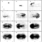
Figure 11: An example of chaotic mixing in a fixed triaxial potential (Merritt & Valluri 1996). An ensemble of $10^{4}$ isoenergetic particles move independently in the time-dependent gravitational field generated by the Imperfect Ellipsoid with $m_{0}=0.01$. Each frame is labelled by the elapsed time in units of the period of the long-axis orbit; the particles are seen in projection against the $x-z$ plane. After $\sim 100$ orbital periods, the particles have reached a nearly stationary, coarse-grained state. This example suggests the way in which time-independent density components exist even in potentials that are not characterized by integrals of the motion aside from the energy.

Similar calculations in three dimensions were carried out in the “imperfect ellipsoid” potential by Merritt & Valluri (1996) (Figure 11). Ensembles of particles were evolved starting from small patches on the equipotential surface, initial conditions that would have generated box orbits in an integrable potential. Merritt & Valluri also found an initially rapid approach to a near-invariant distribution followed by a slower evolution. Ensembles with starting points near the $y-z$ instability strip (Figure 3) exhibited the most rapid mixing, with e-folding times of only $\sim 10$ crossing times in models with small core radii $m_{0}$ or with central point masses containing $\mathrel{\mathchoice{\lower 3.6pt\vbox{\halign{$\mathsurround=0pt\displaystyle\hfil#\hfil$\cr>\crcr\sim\crcr}}}{\lower 3.6pt\vbox{\halign{$\mathsurround=0pt\textstyle\hfil#\hfil$\cr>\crcr\sim\crcr}}}{\lower 3.6pt\vbox{\halign{$\mathsurround=0pt\scriptstyle\hfil#\hfil$\cr>\crcr\sim\crcr}}}{\lower 3.6pt\vbox{\halign{$\mathsurround=0pt\scriptscriptstyle\hfil#\hfil$\cr>\crcr\sim\crcr}}}}0.1\%$ of the total mass. Ensembles started near regions where the motion was regular evolved more slowly, a consequence of the “stickiness” of invariant tori. Merritt & Valluri suggested that chaotic mixing would tend to axisymmetrize at least the central regions of triaxial galaxies with high central concentrations or massive nuclear black holes.

Kandrup (1998a) compared the efficiency of phase mixing and chaotic mixing in 2D and 3D potentials. He noted that – for initially very localized ensembles – the two processes occur at very different rates: chaotic mixing takes place on the Liapunov, or exponential divergence, time scale while the phase mixing rate falls to zero. But phase mixing of a group of points with a finite extent can be much more rapid. Furthermore the mixing rate of chaotic ensembles typically falls below the Liapunov rate once the trajectories separate; this is especially true for those stochastic orbits that are confined over long periods of time to restricted parts of phase space. The effective rates of phase mixing and chaotic mixing might therefore be comparable in real galaxies. Kandrup noted also that chaotic mixing in 3D potentials can occur at substantially different rates in different directions.

Smooth potentials are idealizations of real elliptical galaxies, which sometimes contain imbedded disks, shells, or other fine structure. As seen by a single star, these distortions would add small-amplitude perturbing forces to the mean field. Such perturbations would not be expected to have much consequence for either strongly chaotic or nearly regular orbits, but they might have an appreciable effect on the evolution of weakly stochastic orbits, by scattering trajectories away from a trapped region into a region where mixing is more rapid. Goodman & Schwarzschild (1981) found that small perturbations had relatively little effect on the behavior of stochastic orbits in their nearly-integrable triaxial model. Habib, Kandrup & Mahon (1996, 1997) observed much more striking effects of noise on the evolution of trapped stochastic orbits in two dimensionial potentials. These authors found that even very weak noise, with a characteristic time scale $|{{1\over v}{\delta v\over\delta t}}|^{-1}$ of order $10^{6}$ crossing times, could induce substantial changes in the motion of trapped stochastic orbits over $\sim 10^{2}$ periods. Merritt & Valluri (1996) also considered the effect of noise on chaotic mixing in triaxial potentials. They observed a significant enhancement in the mixing rate of trapped ensembles for noise with a characteristic time scale of $\sim 10^{3}$ orbital periods. These results suggest that chaotic mixing in strongly time-dependent potentials, like those associated with a collapsing protogalaxy, might be much more efficient than in experiments based on fixed potentials.

5.2.3 Mixing in Time-Dependent Potentials

In a real galaxy, the approach to a stationary state takes place against the backdrop of a time-varying potential. King (1962), Hénon (1964), Lynden-Bell (1967) and others realized that relaxation under such conditions might be very efficient, and the latter author made the bold suggestion that the relaxation rate could be directly identified with the rate of change of a star’s potential energy. Lynden-Bell proposed that the time scale for “violent relaxation” was

$$T_{vr}={3\over 4}\langle{\dot{\Phi}^{2}\over\Phi^{2}}\rangle^{-1/2}$$ (34)

with $\dot{\Phi}$ the time derivative of the gravitational potential. For a collapsing sphere, Lynden-Bell noted that $T_{vr}$ was similar to the collapse time, consistent with $N$-body simulations which showed nearly complete relaxation after just a few radial oscillations.

A rearrangement of stars in energy space can only take place if the potential is time-dependent. But in other respects, the identification of $\partial\Phi/\partial t$ with a relaxation rate is problematic. Instantaneous changes in the potential imply only a relabelling of particle energies, not necessarily a divergence of phase space trajectories or a redistribution of energies, which are also prerequisites for relaxation. It is in fact possible to construct oscillating models which exhibit no tendency to relax (Louis & Gerhard (1988); Sridhar (1989); Sridhar & Nityananda (1989); Mineau, Feix & Rouet (1990)). The failure of these models to reach a steady state is a result of their being constructed in such a way that mixing is inhibited; thus the distribution of particle energies does not relax even though the energy of individual particles is constantly changing. For instance, in Sridhar’s (1989) pulsating models, all of the stars move with the same fixed frequencies and no mixing can occur. Such examples are artificial but demonstrate that mixing is no less a prerequisite for relaxation in time-dependent potentials than it is in fixed potentials. Potential fluctuations would be expected to promote relaxation only to the extent that they encourage mixing.

Mixing that is driven by changes in the mean-field potential is self-limiting in the sense that the potential approaches a steady state as the mixing progresses. The effectiveness of “violent relaxation” therefore depends strongly on how long the mixing is able to continue, hence on the initial conditions. A number of numerical simulations have borne this out. Hoffman, Shlosman & Shaviv (1979) followed the collapse and relaxation of a spherical galaxy starting from two initial states with different values of the “virial ratio” $|2T/W|$, where $T$ and $W$ are the initial kinetic and potential energies. For $|2T/W|=0.49$ they found a deeper collapse than for $|2T/W=0.59|$, but the subsequent decay of the virial ratio to its equilibrium value of $1$ was also more rapid, thus allowing less time for the mixing to take place. Van Albada and May (van Albada (1982); May & van Albada (1984)) simulated the evolution of initially “cold” clouds with irregular shapes and clumpy particle distributions. They found that the degree of relaxation – as measured, for instance, by the change in the binding energy distribution – was well correlated with the initial degree of irregularity. They argued that clumpy initial conditions were effective at driving relaxation since they permitted the mixing to continue for a prolonged period of time. Villumsen (1984) carried out similar experiments starting from spherical as well as highly flattened initial conditions. He too noted the greater complexity of the motion in the nonspherical collapses and he argued that this complexity was necessary if the evolving galaxy was to lose memory of its initial state. Similar conclusions were reached by McGlynn (1984) and by Londrillo, Messina & Stiavelli (1991).

The view of relaxation in a time-dependent potential as a self-limiting process was incorporated into a heuristic model by Wiechen, Ziegler and collaborators (Wiechen, Ziegler & Schindler (1988); Ziegler & Wiechen (1989); Stahl, Ziegler & Wiechen (1990); Ziegler & Wiechen (1990)). These authors assumed that the degree to which an out-of-equilibrium stellar system relaxes could be estimated by comparing it to a reference system, the “lowest energy state,” defined in the following way. Starting from the initial state, they rearranged the matter in phase space so as to minimize the total energy; in other words, they required the largest values of $f$ to coincide with the most negative values of $h=v^{2}/2+\Phi$ and vice versa. At the same time, they required that Liouville’s theorem be satisfied, i.e. that the volume of each element of phase space be conserved. Wiechen, Ziegler & Schindler (1988) showed that such a “lowest energy state” could always be uniquely defined. This state is however unreachable, since its energy is (by definition) different from that of the initial state. But Ziegler & Wiechen (1989) suggested that the energy difference between the initial and lowest-energy states could be taken as a measure of the degree to which the potential would evolve before the mixing came to a halt. They then simulated the mixing process by applying a smoothing operator to the initial state, after demonstrating that the smoothing process always increases the total energy by making the distribution of matter less compact. They therefore chose the smoothing length such that the reference model corresponding to the smoothed initial distribution had the same energy as the unsmoothed initial state. Finally they identified this smoothed, lowest energy state with the equilibrium configuration. Ziegler & Wiechen (1989) applied their formalism to a single, spherical initial state and found good agreement with a full numerical simulation.

Nozakura (1992) applied Wiechen & Ziegler’s algorithm to the spherical initial states considered by van Albada (1982) in his $N$-body simulations. Nozakura found that the formalism was useful for predicting the final state when the initial state was only moderately far from equilibrium, with a virial ratio $2T/|W|\mathrel{\mathchoice{\lower 3.6pt\vbox{\halign{$\mathsurround=0pt\displaystyle\hfil#\hfil$\cr>\crcr\sim\crcr}}}{\lower 3.6pt\vbox{\halign{$\mathsurround=0pt\textstyle\hfil#\hfil$\cr>\crcr\sim\crcr}}}{\lower 3.6pt\vbox{\halign{$\mathsurround=0pt\scriptstyle\hfil#\hfil$\cr>\crcr\sim\crcr}}}{\lower 3.6pt\vbox{\halign{$\mathsurround=0pt\scriptscriptstyle\hfil#\hfil$\cr>\crcr\sim\crcr}}}}0.5$, but that the agreement was poor for stronger collapses. Ziegler, Wiechen & Arendt (1994) argued that the mixing in strong collapses was “non-uniform,” i.e. that the appropriate smoothing length to apply to particles in the (final) core and halo should be different. Lacking a detailed understanding of the evolution, however, they were unable to specify how the smoothing length should vary with position. They noted also that the tendency of initially spherical models to acquire highly elongated shapes during the collapse (Merritt & Aguilar (1985); Aguilar & Merritt (1990); Canizzo & Hollister (1992)) had no natural explanation in their model.

Figure 12: Evolution of a spherically-symmetric system of particles in $(r,v_{r})$ phase space starting with zero velocity and $\rho\propto r^{-3/2}$ (Henriksen & Widrow 1997). The initial evolution is similar to phase mixing in spite of the rapidly varying potential; after a certain point, the motion undergoes a transition to a more chaotic flow, allowing rapid mixing between particles on neighboring phase-space streams. This example shows that the distinction made in Figure 10, between phase mixing and chaotic mixing in a fixed potential, is qualitatively valid in time-dependent potentials as well.

An interesting illustration of mixing in a time-dependent potential was presented by Henriksen & Widrow (1997). These authors simulated spherically-symmetric collapses of “cold” particle distributions with power-law density profiles, $\rho\sim r^{-\gamma}$, $0<\gamma<3$. The initial evolution was found to be essentially similar to phase mixing, in spite of the rapidly varying potential: the single phase-space thread corresponding to the initial model became more and more tightly wound as the sphere oscillated (Figure 12). After a certain point, however, the motion underwent a transition to a more complex flow, which allowed rapid mixing between particles on neighboring phase-space streams. While highly idealized, Henriksen & Widrow’s simulations provide a striking illustration of the way in which the efficiency of relaxation is tied more to the complexity of the phase-space flow than to the rate of change of the potential.

5.2.4 Entropy

Mixing in a time-dependent potential allows the energies of stars to change, and if the mixing is very efficient or prolonged, one might expect the distribution of energies to approach a “most probable” state. Much the same thing takes place in a gas, where collisions between molecules imply a rapid exchange of kinetic energies; the most probable distribution of particle energies is obtained by maximizing the entropy, leading to the well-known Maxwell-Boltzmann velocity distribution. One can carry out a similar calculation for stellar systems (Ogorodnikov (1965); Lynden-Bell (1967); Shu (1978)), with the not-very-surprising result that the velocity distribution should be Maxwellian in this case as well. However the self-consistent model corresponding to a Maxwellian velocity distribution, the isothermal sphere, has an infinite radius and mass. One might interpret this to mean that the phase-space structure of a real galaxy should be similar in some respects to that of an isothermal sphere, but the entropy arguments give little indication of precisely what the similarities should be.

A number of authors have nevertheless attempted to use entropy arguments to draw conclusions about the end state of collisionless relaxation (Tremaine, Hénon & Lynden-Bell (1986); Madsen (1987); White & Narayan (1987); Mathur (1988); Spergel & Hernquist (1992); Soaker (1996)). In addition to the difficulty just mentioned, these studies must deal with the fact that the equilibrium state of a stellar system depends strongly on the initial conditions. If the correct final state is to be singled out by an entropy maximization, the dependence of the final state on the initial state must somehow be translated into a set of constraints. Inferring the final state then becomes equivalent to specifying these constraints. There is currently no clear understanding of how this can be done and it is not even certain that the exercise would be physically enlightening.

An illustration of the subtleties associated with entropy arguments is the controversy surrounding the study of Tremaine, Lynden-Bell & Hénon (1986). These authors noted, following Tolman (1938), that any functional of the form

$$S_{C}(f)=-\int C(f)d{\bf x}d{\bf v}$$ (35)

is precisely conserved during collisionless evolution; here $C(f)$ is any “convex” function of $f$, $d^{2}C/df^{2}\geq 0$. The constancy of $S_{C}$ is a result of the detailed conservation of phase space volume implied by Liouville’s theorem. However if one computes $S_{C}$ at some time $t_{2}$ using a coarse-grained approximation to $f$, and compares it to the value of $S_{C}$ computed at an earlier time $t_{1}$ using the exact $f$, one finds

$$S_{C}(t_{2})>S_{C}(t_{1}).$$ (36)

One is tempted to conclude that $S_{C}$ is a monotonically increasing function of time and that any such functional can play the role of an entropy. Such a conclusion was rejected by a number of authors (Binney (1987); Dejonghe (1987); Kandrup (1987); Sridhar (1987)) on the following grounds. Identifying the initial state with the fine-grained $f$ is equivalent to assuming that the initial state is known with infinite precision. The increase in $S_{C}$ is then a consequence of the coarse-graining: at any time, the coarse-grained $S_{C}$ is greater than the fine-grained $S_{C}$, hence $S_{C}(t_{2})>S_{C}(t_{1})$. But it does not follow that $S_{C}$ is monotonically increasing and it might well decrease. In fact, equation (36) is true irrespective of whether $t_{2}$ is greater or less than $t_{1}$.

Entropy increases of a physically interesting sort are always associated with irreversibility, that is with chaos (Ruelle (1991)), and it is remarkable that so few discussions of entropy in the galactic dynamics literature have paid any attention to the dynamical properties of the phase-space flow. Chaotic mixing in a fixed potential, as illustrated in Figure 11, represents a true entropy increase in the sense understood by Boltzmann, and the irreversibility observed in numerical simulations of “violent relaxation” (e.g. Figure 12) suggests that something very similar takes place in time-dependent potentials as well. It is in this direction that a fuller understanding of collisionless relaxation probably lies.

5.3 Mixing-Induced Evolution

The irreversibility of mixing flows like the one illustrated in Figure 11 implies a reduction in the effective number of orbits: all the stochastic trajectories at a given energy are gradually replaced by a single invariant ensemble, whose shape is typically not well matched to that of the galaxy. If time scales for chaotic mixing are comparable to galaxy lifetimes, this reduction might be expected to encourage a galaxy to evolve away from a triaxial shape toward a more axisymmetric one, in which most of the orbits are tubes that avoid the destabilizing center.

A pioneering study of mixing-induced evolution was carried out by Norman, May & van Albada (1985), who performed $N$-body integrations of triaxial models in which a central compact object was slowly grown. They found a modest degree of evolution toward more spherical shapes near the center. Norman et al.’s simulations were intended to represent the effect of a massive nuclear black hole on the surrounding galaxy; however, because of computational limitations, they were forced to adopt a softening length for the central object that was close to the gravitational radius of influence $r_{h}\sim GM_{h}/\sigma^{2}$ of a true point mass. In addition, their initial models were chosen to be close to axisymmetric. As Norman et al. noted, both of these factors would tend to limit the evolution, the first by eliminating large-angle scattering of trajectories by the central object, the second by reducing the fraction of stars on boxlike orbits that could pass near the center.

A natural way to increase the central density of a galaxy model is through the inclusion of a dissipative component which accumulates near the center as its energy and angular momentum are carried away. $N$-body studies of galaxy formation that include such a component often reveal an evolution toward more axisymmetric shapes as the central mass grows. Katz & Gunn (1991) carried out such simulations starting from initial conditions containing either no “gas,” or a $10:1$ ratio of “stellar” to “gas” particles. Initially the two components were well mixed; however the gas particles quickly accumulated near the center where they formed a disk. In the absence of a dissipative component, the stellar particles in these simulations relaxed into strongly triaxial shapes, with typical axis ratios of $\sim 1:0.7:0.5$. When gas was included, the final stellar distribution was found to always be nearly oblate-axisymmetric, with $b/a\mathrel{\mathchoice{\lower 3.6pt\vbox{\halign{$\mathsurround=0pt\displaystyle\hfil#\hfil$\cr>\crcr\sim\crcr}}}{\lower 3.6pt\vbox{\halign{$\mathsurround=0pt\textstyle\hfil#\hfil$\cr>\crcr\sim\crcr}}}{\lower 3.6pt\vbox{\halign{$\mathsurround=0pt\scriptstyle\hfil#\hfil$\cr>\crcr\sim\crcr}}}{\lower 3.6pt\vbox{\halign{$\mathsurround=0pt\scriptscriptstyle\hfil#\hfil$\cr>\crcr\sim\crcr}}}}0.9$. The short-to-long axis ratio was nearly unchanged. Udry (1993) simulated dissipation in triaxial galaxy models by a number of schemes: including an ad hoc drag force on $10\%$ of the particles; adding a central particle containing $2.5\%$ of the stellar mass; or including a centrally concentrated distribution of particles containing $5\%$ or $10\%$ of the total mass. While the simulations without “dissipation” resulted in models with a range of triaxialities, the simulations including dissipation evolved to nearly axisymmetric shapes, with $0.7\mathrel{\mathchoice{\lower 3.6pt\vbox{\halign{$\mathsurround=0pt\displaystyle\hfil#\hfil$\cr<\crcr\sim\crcr}}}{\lower 3.6pt\vbox{\halign{$\mathsurround=0pt\textstyle\hfil#\hfil$\cr<\crcr\sim\crcr}}}{\lower 3.6pt\vbox{\halign{$\mathsurround=0pt\scriptstyle\hfil#\hfil$\cr<\crcr\sim\crcr}}}{\lower 3.6pt\vbox{\halign{$\mathsurround=0pt\scriptscriptstyle\hfil#\hfil$\cr<\crcr\sim\crcr}}}}b/a\mathrel{\mathchoice{\lower 3.6pt\vbox{\halign{$\mathsurround=0pt\displaystyle\hfil#\hfil$\cr<\crcr\sim\crcr}}}{\lower 3.6pt\vbox{\halign{$\mathsurround=0pt\textstyle\hfil#\hfil$\cr<\crcr\sim\crcr}}}{\lower 3.6pt\vbox{\halign{$\mathsurround=0pt\scriptstyle\hfil#\hfil$\cr<\crcr\sim\crcr}}}{\lower 3.6pt\vbox{\halign{$\mathsurround=0pt\scriptscriptstyle\hfil#\hfil$\cr<\crcr\sim\crcr}}}}1$. Dubinski (1994) simulated dissipative infall inside an initially triaxial halo by slowly increasing the mass associated with a central, fixed component having either a spherical or disklike shape. The final mass of this central object was $\sim 5\%$ the mass of the surrounding halo; however its scale length was large, roughly $0.1$ that of the halo. Dubinski nevertheless found a modest increase in the intermediate-to-long axis ratio of the halo, from $\sim 0.6$ to $\sim 0.8$, with less change in $c/a$.

Barnes (1992, 1996) reported the results of $N$-body simulations of mergers between disk galaxies with and without a dissipative component. In the absence of gas, the remnants acquired shapes that depended strongly on the initial orientations and impact parameter of the colliding disks; many of the remnants were strongly triaxial. When as little as $1.5\%$ of the total mass was added in the form of dissipative particles, the remnants acquired much more axisymmetric shapes. Barnes (1996) cataloged the stellar orbits in the remnants and found a preponderance of short-axis tubes in the remnants containing gas, as expected for nearly axisymmetric potentials. Barnes & Hernquist (1996) confirmed these results with further simulations and noted that the final shapes of the remnants were well correlated with the depth of the central potential. They speculated that the evolution toward oblate figures was driven largely by the destabilization of box orbits moving in the deepened potential, i.e. by chaotic mixing.

The effect of a massive central singularity on the structure of an initially triaxial galaxy was studied by Merritt & Quinlan (1998) using an $N$-body code with much higher spatial and temporal resolution than in the pioneering simulation of Norman et al. The final shape achieved by their model after growth of the black hole was nearly spherical at the center and close to axisymmetric throughout; the rate of change of the galaxy’s shape depended strongly on the ratio $M_{h}/M_{g}$ of black hole mass to galaxy mass. When $M_{h}/M_{g}$ was less than about $0.3\%$, the galaxy evolved in shape over $\sim 10^{2}$ orbital periods, while increasing $M_{h}/M_{g}$ to $3\%$ caused the galaxy to become axisymmetric in little more than a crossing time. Merritt & Quinlan proposed that the rapid evolution toward axisymmetric shapes for $M_{h}/M_{g}\mathrel{\mathchoice{\lower 3.6pt\vbox{\halign{$\mathsurround=0pt\displaystyle\hfil#\hfil$\cr>\crcr\sim\crcr}}}{\lower 3.6pt\vbox{\halign{$\mathsurround=0pt\textstyle\hfil#\hfil$\cr>\crcr\sim\crcr}}}{\lower 3.6pt\vbox{\halign{$\mathsurround=0pt\scriptstyle\hfil#\hfil$\cr>\crcr\sim\crcr}}}{\lower 3.6pt\vbox{\halign{$\mathsurround=0pt\scriptscriptstyle\hfil#\hfil$\cr>\crcr\sim\crcr}}}}2.5\%$ would tend to cut off the supply of fuel to a growing black hole, thus imposing an upper limit to its mass.

Chaotic mixing induced by a central density cusp or nuclear black hole could have a number of other consequences for the structure of elliptical galaxies and bulges (Merritt (1998)). Elliptical galaxies with nonsmooth phase space populations are expected to be “boxy” or peanut-shaped, since individual orbits, both boxes and tubes, are strongly dimpled when seen in projection (Binney & Petrou (1985)). The fact that most elliptical galaxies have accurately elliptical isophotes suggests that some process has acted to smooth the distribution of orbital turning points at every energy. “Violent relaxation” is one candidate for this smoothing process, but it is apparently not effective enough, since the end-products of $N$-body simulations are often strongly peanut-shaped (e.g. May, van Albada & Norman (1985); Quinn & Goodman (1986); Udry (1993); Ziegler, Wiechen & Arendt (1994)). An alternative mehcanism is chaotic mixing induced by a central black hole; Merritt & Quinlan (1998) noted that the growth of a central mass concentration converts boxy, triaxial systems into axisymmetric ones with accurately elliptical isophotes. This result may explain the observed correlation between boxiness and kinematical measures of triaxiality (Kormendy & Bender (1996)). On a deeper level, the distribution function of an axisymmetric galaxy formed in this way would be biased toward forms for $f$ that are as nearly constant as possible, i.e. which do not depend strongly on a third integral. Detailed modelling of M32, a galaxy that is old compared to expected time scales of chaotic mixing, in fact suggests a best-fit $f\approx f(E,L_{z})$ (van der Marel et al. (1998)).

6 COLLECTIVE INSTABILITIES

The chaotic mixing discussed in the previous section is driven by the exponential instability of stochastic motion; the effect of such mixing is typically to erase a density perturbation by spreading particles in phase space. However it is possible for a density perturbation to grow by inducing motion that reinforces the original overdensity. Such collective instabilities typically require the unperturbed motion to be highly correlated and they have been most thoroughly studied in thin disks, which are subject to a variety of unstable modes when sufficiently “cold” (Sellwood & Wilkinson (1993)). In elliptical galaxies, where the stellar motions are more nearly random in direction, a perturbation in the density might be expected to rapidly attenuate as the stars move along their respective orbits. However it turns out that the motion in a variety of physically reasonable models is sufficiently correlated to induce growing modes.

The simplest model for an elliptical galaxy is a sphere in which the stellar velocities are isotropic, $f=f(E)$. Antonov (1960, 1962) established a necessary and sufficient condition for linear stability of spherical systems satisfying $df/dE<0$, in the form of a complicated variational principle. He went on to derive a number of simpler, sufficient conditions for stability. The most important of these are:

I. A spherical system with $f=f(E)$ and $df/dE<0$ is stable to all non-radial (i.e. non-spherically-symmetric) perturbations.

II. A spherical system with $f=f(E)$, $df/dE<0$ and $d^{3}\rho/d\Phi^{3}\leq 0$ is stable to all perturbations.

Antonov was able to show that the family of “stellar dynamical polytropes” defined by

$$f(E)=f_{0}(E_{0}-E)^{n-3/2},\ \ \ \ E\leq E_{0},$$ (37)

is stable for $n\geq 3/2$, i.e. for all values of $n$ such that $df/dE\leq 0$. Antonov’s second theorem was generalized by Doremus, Feix & Baumann (1971), Sygnet et al. (1984) and Kandrup & Sygnet (1985) to include any spherical system with $df/dE<0$. This result may be used to verify that many of the isotropic models that resemble real galaxies are linearly stable.

A number of attempts have been made to generalize Antonov’s theorems to spherical systems with anisotropic velocities, $f=f(E,L^{2})$. One such generalization follows directly from Theorem II above: stability to radial perturbations is guaranteed if $\left({\partial\over\partial E^{*}}\right)^{2}\int_{E^{*}}^{0}f(E,L^{2}){dE\over(E-E^{*})}<0$ (Dejonghe & Merritt (1988)). Theorems of an even more general nature have been proposed, but their validity is not always clear. Dorémus & Feix (1973) and Gillon, Doremus & Baumann (1976) analyzed a “water bag” model for spherical stellar systems, in which the distribution function is represented as a set of bags of incompressible fluid; a perturbation is interpreted as a change in the volumes of the bags rather than as a change in the numerical value of the distribution function. They found stability to radial perturbations when $\partial f/\partial E<0$ and stability to all perturbations when $\partial f/\partial L<0$ as well. The former result was confirmed by Kandrup & Sygnet (1985) and Perez & Aly (1996), but the latter result would seem to definitely contradict numerical studies of the radial-orbit instability described below (§6.2); in fact Perez & Aly were able to find an error in the Gillon et al. proof. A criterion proposed by Hjorth (1994) for stability of a certain class of anisotropic models is also inconsistent with numerical results (Meza & Zamorano (1997)).

As an alternative to proving theorems on stability, one can use physical intuition to search for particular, unstable models. This approach has been extremely successful, leading to the identification of several types of unstable behavior in models of hot stellar systems. Results on four such instabilities are reviewed below, roughly in the order in which their importance was first recognized. The first is a pulsational instability of spherical systems, first reported by Hénon (1973). The second is the radial-orbit instability, postulated by Antonov (1973) and observed by Polyachenko (1981). Third are bending instabilities, described as early as 1966 by Toomre in the context of disks, and observed in a number of $N$-body studies starting around 1990. Finally, instabilities in slowly-rotating oblate models with nearly circular orbits are discussed; these instabilities were first noticed in disk models and later seen in oblate spheroids.

6.1 Hénon’s instability

Antonov’s proofs leave open the question of the stability of systems with anisotropic or non-monotonic distribution functions. Hénon (1973) carried out the first systematic search for instabilities in anisotropic spherical models. He found that the polytropic models defined by equation (37) were stable to spherically symmetric modes, with the possible exception of the $n=1/2$ model, which appeared to oscillate at a level slightly above the noise. (The $n=1/2$ model is extreme in the sense that all stars have exactly the same energy.) Barnes, Goodman & Hut (1986) later established the stability of these models to non-spherical modes as well. Hénon went on to test the stability to radial perturbations of the “anisotropic polytropes” defined by

$$f(E,L^{2})=f_{0}L^{-2m}(E_{0}-E)^{n-3/2}.$$ (38)

Models generated from equation (38) have velocity ellipsoids with fixed axis ratios $\sigma_{r}^{2}/\sigma_{t}^{2}=(1-m)^{-1}$, where $\sigma_{r}$ and $\sigma_{t}$ are the 1D, radial and tangential components of the velocity dispersion tensor. Hénon found that the oscillatory instability that seemed to be present in the isotropic model with $n=1/2$ became stronger as the velocity ellipsoid was made more prolate. He mapped out the region of instability in the $(m,n)$-plane and found that models with $n$ as large as $\sim 1$ could be unstable when the velocity ellipsoid was sufficiently elongated.

Barnes, Goodman & Hut (1986) reanalyzed the stability of the anisotropic polytropes using a more sophisticated $N$-body code. They confirmed Hénon’s results and noted that the instability boundary for radial modes could be approximated by $n-m=1/2$, suggesting instability even for $n=3/2$ when the orbits were fully radial. Barnes et al. noted that the stability boundary coincided roughly with the condition that the distribution of radial velocity have two peaks, and suggested that the “two-stream” nature of the velocity distribution was a necessary condition for this instability. They noted further that $\partial f/\partial E>0$ was a requirement for a spherical model to have such a double-peaked distribution. Neither Hénon nor Barnes et al. discussed in detail the structure of their unstable models after they had reached a steady state, although the major effect of the instability seemed to be a radial spreading of stars.

The two conditions for instability established by these studies – $\partial f/\partial E>0$, and radially-elongated velocity ellipsoids – imply an equilibrium density profile that diverges near the center, roughly as a power law. Until recently, such a density dependence was considered unphysical, but it is now known that early-type galaxies always have power-law density cusps (Merritt & Fridman (1995); Gebhardt et al. (1996)). Further work on Hénon’s instability would therefore be useful.

6.2 The radial-orbit instability

Antonov (1973) suggested that a spherical model constructed from purely radial orbits would be unstable to clumping of particles around any radius vector. The instability was verified numerically by Polyachenko (1981), who followed the evolution of a 200-particle radial-orbit model into a bar. Barnes (1985) rediscovered the instability while using an $N$-body code to test the stability of Hénon’s generalized polytropes; he observed growing barlike distortions in radially anisotropic models with a wide range of $m$’s and $n$’s.

The instability is similar to one first described by Lynden-Bell (1979) in the context of radially-hot disks. In spherical systems with well-behaved central potentials, elongated orbits are nearly closed, making slightly less than two radial oscillations for each circulation in angle. Such an orbit acts like a slowly precessing ellipse, or rod (Polyachenko (1989)); the precession rate tends to zero for low $L$. In the presence of a barlike perturbation to the potential, an elongated orbit experiences a torque which causes it to precess more rapidly toward the bar; after passing through the bar, the orbit loses angular momentum and precesses more slowly. The result is an enhancement of the density in the neighborhood of the bar.

The strength of the instability, and its effect on the shapes of initially spherical models, were explored in a number of $N$-body studies. Merritt & Aguilar (1985) examined the stability of models with Dehnen’s density law, $\gamma=2$, and three different types of distribution function. They noted that the behavior of the instability depended sensitively on the low-$L$ dependence of $f$. In models where the phase-space density was divergent at low $L$ (as in Hénon’s anisotropic polytropes), the growth rate of the instability and the final ellipticity of the model were found to be gradually increasing functions of the anisotropy. Even very mildly anisotropic models constructed from such distribution functions were found to be unstable. Barnes, Goodman & Hut (1986) reported similar behavior in their $N$-body study of Hénon’s polytropes. Merritt & Aguilar also investigated a family of models generated from a distribution function of the form $f=f(Q),Q=E+L^{2}/2r_{a}^{2}$, in which the phase-space density is constant on spheroids in velocity space and everywhere finite. The latter models are characterized by a central region, $r\mathrel{\mathchoice{\lower 3.6pt\vbox{\halign{$\mathsurround=0pt\displaystyle\hfil#\hfil$\cr<\crcr\sim\crcr}}}{\lower 3.6pt\vbox{\halign{$\mathsurround=0pt\textstyle\hfil#\hfil$\cr<\crcr\sim\crcr}}}{\lower 3.6pt\vbox{\halign{$\mathsurround=0pt\scriptstyle\hfil#\hfil$\cr<\crcr\sim\crcr}}}{\lower 3.6pt\vbox{\halign{$\mathsurround=0pt\scriptscriptstyle\hfil#\hfil$\cr<\crcr\sim\crcr}}}}r_{a}$, in which the motion is nearly isotropic and an outer envelope where the motion becomes increasingly radial (Osipkov (1979); Merritt (1985)). Merritt & Aguilar found that the instability appeared suddenly in these models when $r_{a}$ fell below a critical value, roughly $0.3$ times the half-mass radius. The neutrally-stable model from this family had a global anisotropy ratio $2T_{r}/T_{t}\approx 2.3$, with $T_{r}$ and $T_{t}$ the kinetic energies in radial and tangential motions respectively.

Much of the subsequent work on the radial orbit instability has focussed on models with $f=f(Q)$. Meza & Zamorano (1997) extended the Merritt & Aguilar study to include Dehnen models with a variety of cusp slopes $\gamma$. They found a mild dependence of the critical anisotropy ratio $2T_{r}/T_{t}$ on $\gamma$, from $\sim 2.0$ when $\gamma=2$ (slightly less than the value found by Merritt & Aguilar for the same family) to $\sim 2.6$ for $\gamma=0$. May & Binney (1986) used an adiabatic deformation technique to evaluate the stability of models with $f=f(Q)$ and the isochrone density law. They estimated a critical value of $\sim 2.2$ for the anisotropy ratio. Dejonghe & Merritt (1988) found $(2T_{r}/T_{t})_{crit}\approx 1.9$ in $f=f(Q)$ models with the Plummer density law. Bertin & Stiavelli (1989) used an $N$-body code to test the stability of models with distribution functions of the form $f\propto|E|^{3/2}\exp(aQ)$, designed to represent galaxies that form via radial collapse (Stiavelli & Bertin (1985); Merritt, Tremaine & Johnstone (1989)). They found $(2T_{r}/T_{t})_{crit}\approx 1.9$. Stiavelli & Sparke (1991) derived a very similar criterion for instability in models with $f\propto|E|^{3/2}\exp(aE)/(1+cL^{2})$. Perez et al. (1996) noted the presence of the instability in $f=f(Q)$ models with the density profiles of isotropic polytropes. However they did not look closely at the critical parameter values defining the onset of the instability. Allen, Palmer & Papaloizou (1990) also noted the existence of the instability in an $N$-body study of modified polytropes but did not attempt to establish the stability boundary.

The existence of slowly-growing modes in models with very small global anisotropies, reported by Merritt & Aguilar (1985) and Barnes, Goodman & Hut (1986), calls into question the usefulness of diagnostics like $2T_{r}/T_{t}$ for judging instability. Palmer & Papaloizou (1987) showed that instability to barlike modes is in fact guaranteed in models where $f$ is unbounded at small $L$, regardless of the degree of velocity anisotropy. These results prompted an analysis of the stability of a model of the giant elliptical galaxy M87 constructed by Newton & Binney (1984); their model is close to isotropic except near the center, where $f$ increases rapidly at small $L$. The model was found to be mildly unstable to a barlike mode (Merritt 1987b ).

An alternative to $N$-body techniques when evaluating the stability of equilibrium models is Kalnajs’s (1972) matrix algorithm, which yields numerical expressions for the normal modes and their growth rates. Kalnajs’s algorithm is in principle superior to $N$-body techniques when searching for the exact stability boundary in a family of models, but in practice the eigenvalue equation can be difficult to solve with accuracy when the growth rate is small. Polyachenko & Shukhman (1984) pioneered this approach in the study of spherical systems, deriving the lowest-order modes for a family of nearly-homogeneous models derived by Osipkov. They found instability for $2T_{r}/T_{t}\mathrel{\mathchoice{\lower 3.6pt\vbox{\halign{$\mathsurround=0pt\displaystyle\hfil#\hfil$\cr>\crcr\sim\crcr}}}{\lower 3.6pt\vbox{\halign{$\mathsurround=0pt\textstyle\hfil#\hfil$\cr>\crcr\sim\crcr}}}{\lower 3.6pt\vbox{\halign{$\mathsurround=0pt\scriptstyle\hfil#\hfil$\cr>\crcr\sim\crcr}}}{\lower 3.6pt\vbox{\halign{$\mathsurround=0pt\scriptscriptstyle\hfil#\hfil$\cr>\crcr\sim\crcr}}}}1.6$. Results for two additional families – Hénon’s generalized polytropes, equation (38), and a family of models based on Plummer’s density law – were reported by Fridman & Polyachenko (1984). For the first family, a critical anisotropy ratio $\sim 1.4$ was quoted; however Palmer & Papaloizou (1987) proved that all radially-anisotropic models from this family would be unstable. For the second family, Fridman & Polyachenko found $(2T_{r}/T_{t})_{crit}\approx 1.5$; Dejonghe & Merritt (1988), in an $N$-body study, found instability in this family for $(2T_{r}/T_{t})_{crit}\mathrel{\mathchoice{\lower 3.6pt\vbox{\halign{$\mathsurround=0pt\displaystyle\hfil#\hfil$\cr>\crcr\sim\crcr}}}{\lower 3.6pt\vbox{\halign{$\mathsurround=0pt\textstyle\hfil#\hfil$\cr>\crcr\sim\crcr}}}{\lower 3.6pt\vbox{\halign{$\mathsurround=0pt\scriptstyle\hfil#\hfil$\cr>\crcr\sim\crcr}}}{\lower 3.6pt\vbox{\halign{$\mathsurround=0pt\scriptscriptstyle\hfil#\hfil$\cr>\crcr\sim\crcr}}}}1.9$.

Some of these inconsistencies can be attributed to the difficulties of implementing Kalnajs’s technique. In a very convincing study, Saha (1991) derived the lowest-order unstable models for the family of anisotropic, $f=f(Q)$ isochrone models first analyzed by May & Binney (1986). Saha found instability for $2T_{r}/T_{t}>1.4$, substantially smaller than May & Binney’s estimate of 2.2; this result suggests that spherical models may be unstable over a much wider range of anisotropies than the $N$-body studies indicate. Saha (1992) went on to analyze a second family of isochrone models with a two-parameter distribution function; the first parameter $r_{a}$ defined the size of the isotropic core, while the second parameter $\beta_{\infty}$ fixed the degree of anisotropy at large radii. Saha found a critical anisotropy ratio that ranged from $2T_{r}/T_{t}\approx 2.3$ in models whose envelopes contained purely radial orbits to $\sim 1.8$ in models where the asymptotic anisotropy was $\sigma_{r}/\sigma_{t}\approx 1.6$. Weinberg (1991) derived the unstable modes for $f=f(Q)$ models with the density profiles of isotropic Michie-King models; the latter constitute a one-parameter sequence characterized by the value of the dimensionless central potential $W_{0}$ (King 1966). Weinberg demonstrated instability for low $r_{a}$ in models with several different values of $W_{0}$. For $W_{0}=5$, he found a critical anisotropy radius of $r_{a}\approx 1.2$ in units of the King core radius. Bertin et al. (1994) evaluated the stability of the Stiavelli-Bertin (1985) models and found $(2T_{r}/T_{t})_{crit}\approx 1.6$, substantially less than in the earlier $N$-body study of Bertin & Stiavelli (1989).

These normal-mode calculations suggest that spherical models with $2T_{r}/T_{t}\mathrel{\mathchoice{\lower 3.6pt\vbox{\halign{$\mathsurround=0pt\displaystyle\hfil#\hfil$\cr>\crcr\sim\crcr}}}{\lower 3.6pt\vbox{\halign{$\mathsurround=0pt\textstyle\hfil#\hfil$\cr>\crcr\sim\crcr}}}{\lower 3.6pt\vbox{\halign{$\mathsurround=0pt\scriptstyle\hfil#\hfil$\cr>\crcr\sim\crcr}}}{\lower 3.6pt\vbox{\halign{$\mathsurround=0pt\scriptscriptstyle\hfil#\hfil$\cr>\crcr\sim\crcr}}}}2.3$ are generally unstable, and that models with distribution functions that increase rapidly toward small $L$ can be unstable for much lower values of the mean anisotropy. A model with $2T_{r}/T_{t}=2.3$ has an average ratio of radial to tangential velocity dispersions of $\sigma_{r}/\sigma_{t}\approx 1.5$; thus, one might expect to never see more extreme anisotropies in spherical galaxies. One of the few galaxies for which the anisotropy has been convincingly measured is M87 (van der Marel (1994); Merritt & Oh (1997)), where $\sigma_{r}/\sigma_{t}\approx 1.5$ over a wide range in radius.

The radial-orbit instability would be expected to persist in axisymmetric models with radially-elongated velocity ellipsoids. Levison, Duncan & Smith (1990) reported barlike modes in highly flattened ($c/a\approx 0.4$) oblate models when the radial velocity dispersion exceeded $\sim 0.7$ times the velocity disperision perpendicular to the meridional plane. This result suggests that the radial-orbity instability might be very effective in flattened models; it would be useful to verify the result in an independent study.

Elliptical galaxies often contain central mass concentrations which could strongly influence the elongated orbits that drive the radial-orbit instability. Palmer & Papaloizou (1988) discussed the effect of a central point mass on the instability of models with distribution functions peaked near $L=0$. They noted that a central point mass greatly increases the precession rate of low-$L$ orbits; at a given energy, there is a minimum precession rate corresponding to orbits with a certain nonzero $L$. If this minimum precession rate is larger, for most orbits, than the rate at which a barlike mode would grow in the model without a central point mass, they argued that the instability would be inhibited. Preliminary $N$-body simulations suggested a critical mass of the central object of roughly $0.1\%$ the mass of the model, similar to the masses inferred for the nuclear black holes in a number of galaxies. Given the likely ubiquity of black holes in elliptical galaxies, more work along the lines of Palmer & Papaloizou’s would be valuable.

Polyachenko (1981) noted that collapse from cold initial conditions tends to produce equilibrium systems with strong radial anistropies, and he pointed out that such systems would be unstable to nonspherical modes. He went on to verify (Polyachenko (1985), 1992) the evolution of initially cold and spherical $N$-body clouds into bars. A number of subsequent studies have shown that a wide range of initial conditions can produce collapses where the radial-orbit instability is active. Merritt & Aguilar (1985) found that intially spherical clouds with an $r^{-1}$ density profile evolved into triaxial bars when $(2T/|W|)_{0}$ was less than about 0.2, with $T$ and $W$ the total kinetic and potential energies of the initial configuration. The final elongation was found to increase smoothly with decreasing initial “temperature”; the coldest initial conditions produced models with a final axis ratio of $\sim 2.5:1$. The instability was also found to reduce the central concentration of the relaxed models. Min & Choi (1989) also found a critical virial ratio of $\sim 0.2$ in collapses starting from homogeneous initial conditions. Aguilar & Merritt (1990) extended their earlier work to flattened and rotating initial conditions. They found that collapses with $(2T/|W|)_{0}\mathrel{\mathchoice{\lower 3.6pt\vbox{\halign{$\mathsurround=0pt\displaystyle\hfil#\hfil$\cr<\crcr\sim\crcr}}}{\lower 3.6pt\vbox{\halign{$\mathsurround=0pt\textstyle\hfil#\hfil$\cr<\crcr\sim\crcr}}}{\lower 3.6pt\vbox{\halign{$\mathsurround=0pt\scriptstyle\hfil#\hfil$\cr<\crcr\sim\crcr}}}{\lower 3.6pt\vbox{\halign{$\mathsurround=0pt\scriptscriptstyle\hfil#\hfil$\cr<\crcr\sim\crcr}}}}0.1$ produced final shapes that were nearly uncorrelated with initial shapes; this characteristic final shape was approximately prolate with a $2:1$ axis ratio. The minimum amount of rotation required to inhibit the bar instability was found to be $\lambda\approx 0.1$, with $\lambda$ the standard dimensionless spin parameter. Cannizzo & Hollister (1992) explored the dependence of the final shape of a collapsing cloud on its initial density profile. They distributed particles according to $\rho\propto r^{-n}$ initially with $0<n<2.5$ and set the virial ratio to a very low value, $(2T/|W|)_{0}\approx 0.01$. Their final configurations were approximately prolate, with axis ratios that varied from $\sim 1.8:1$ for $n=2.5$ to $\sim 1.3:1$ for $n=0$. Theis & Spurzem (1998) carried out a series of direct-summation $N$-body collapse simulations using large numbers of particles ($N\approx 3\times 10^{4}$) and small softening lengths. Particles were initially distributed according to Plummer’s law, with $2T/W\approx 0.04$. The final models were prolate/triaxial and very elongated, with $c/a\approx 0.4-0.5$.

As a number of authors have noted, the final elongations of these models are close to the maximum value permitted by the bending instability discussed below. Polyachenko (1992) suggested that the distribution of elliptical galaxy axis ratios might be determined by the competition between these two instabilities. However recent determinations of the frequency function of elliptical galaxy intrinsic shapes (Tremblay & Merritt (1995), 1996; Ryden (1996)) find a peak near $c/a\approx 0.8$, too round to be convincingly explained in this way.

6.3 Bending instabilities

Toomre (1966) showed that a thin stellar sheet has a tendency to buckle when the stars have large random velocities along the plane and are constrained to remain in a single thin layer as the sheet bends. The constraining force comes from the vertical self-gravity of the sheet, which is large if the sheet is thin. Stars moving across a bend are forced to oscillate vertically as they pursue their unperturbed horizontal motions, and the bend will grow if the gravitational restoring forces from the perturbation are too weak to provide the vertical acceleration required. The thin-sheet dispersion relation is (Toomre 1966)

$$\omega^{2}=2\pi G\Sigma k-\sigma_{x}^{2}k^{2}$$ (39)

where $\sigma_{x}$ is the velocity dispersion parallel to the sheet and $\Sigma$ is its surface density. The first term, which arises from the perturbed gravity, is stabilizing, while the second term, due to the centrifugal force that the stars exert on the sheet, is destabilizing. Because the stabilizing force decreases less rapidly with the wavelength of the bend than does the destabilizing force ($\lambda^{-1}$ vs. $\lambda^{-2}$), short-wavelength perturbations are the most unstable. For sufficiently long wavelengths $\lambda>\lambda_{J}=\sigma_{x}^{2}/G\Sigma$, the gravitational restoring force dominates and the sheet is stable. Bending instabilities are precisely complementary, in this sense, to the Jeans instability in the plane, which is stabilized at wavelengths $\lambda<\lambda_{J}$. Toomre’s analysis, which was based on the moment equations, was shown by Mark (1971) and Kulsrud, Mark & Caruso (1971) to be valid for slabs of arbitrary vertical structure whenever the wavelength of the perturbation greatly exceeds the thickness of the slab.

At wavelengths shorter than the actual vertical thickness of the layer, Toomre argued that the bending would once again be stabilized. Since the thickness of a slab scales as $\sigma_{z}^{2}/G\Sigma$, with $\sigma_{z}$ the vertical dispersion, Toomre noted that both long- and short-wavelength perturbations should be stabilized when $\sigma_{z}/\sigma_{x}$ was sufficiently large. He estimated a critical value of $0.30$ for this ratio. Polyachenko & Shukhman (1977) found a very similar value for the critical anisotropy in a homogenous slab, for which the bending takes the form of surface corrugations. Araki (1985) computed the exact linear normal modes of a finite-thickness slab with an anisotropic Gaussian velocity distribution. He found that bending at all wavelengths was stabilized when the ratio of vertical to horizontal velocity dispersions exceeded $\sim 0.293$, remarkably close to Toomre’s earlier estimate. At the instability threshold, the single, neutrally-unstable mode has a wavelength of about 1.2 in units of $\lambda_{J}$.

The elongation of a pressure-supported galaxy with the Toomre-Araki critical anisotropy is approximately $1:15$, which would seem to suggest that bending modes are unlikely to be important in structuring elliptical galaxies. But a number of subsequent studies revealed instability in much rounder models. Polyachenko & Shukhman (1979) and Vandervoort (1991) calculated the exact linear normal modes for constant-density stellar spheroids, both oblate and prolate. In models where the distribution function favored radial motions, both studies found critical axis ratios of $\sim 1:3$, not $\sim 1:15$. Merritt & Hernquist (1991) carried out an $N$-body study of inhomogeneous prolate models; they also found a critical axis ratio of $0.3-0.4$.

Figure 13: Bending instability in a prolate, “shell-orbit” model (Merritt & Hernquist 1991). The initial model has axis ratio $c/a=0.1$; frames are separated by $\sim 4$ periods of the long-axis orbit. The dominant mode is an antisymmetric bend that induces a long-lived peanut shape. Prolate models with elongations more extreme than $\sim 3:1$ are found to be unstable to bending modes.

The discrepancy was explained in the following way (Merritt & Sellwood (1994)). In finite or inhomogenous models, the gravitational restoring force from the bend – represented by the first, stabilizing term in equation (39) – is substantially weaker than in infinite sheets and slabs. In fact, bending modes in thin systems with realistic density profiles are often not stabilized by gravity even at the longest wavelengths. However bending modes can still be stabilized in such systems, for the following reason. Stars in a finite-thickness system oscillate vertically with an unperturbed frequency $\kappa_{z}$; like any oscillator, the phase of a star’s response to the imposed bending depends entirely on whether the forcing frequency $kv_{x}$ is greater than or less than its natural frequency. If $kv_{x}>\kappa_{z}$ for most stars, the overall density response to the perturbation will produce a potential opposite to that imposed by the bend and the disturbance will be damped. Merritt & Sellwood showed that this mechanism was responsible for the short-wavelength stabilization found by Toomre (1966) and Araki (1985) in the infinite slab. In a finite or inhomogeneous stellar spheroid, where the gravitational restoring force from the bend is much smaller than in an infinite slab, almost all of the stabilization is due to this out-of-phase damping. Since a typical star in such a system feels a vertical forcing frequency from a long-wavelength bend that is roughly twice the frequency $\omega_{x}$ of its orbital motion along the long axis, stability to global modes requires that the forcing frequency be less than $\omega_{z}$, the frequency of orbital motion along the short axis. The resulting condition $2\omega_{x}>\omega_{z}$ predicts stability for a pressure-supported, homogeneous prolate spheroid rounder than $\sim 1:2.94$, in excellent agreement with the normal-mode calculations of and Fridman & Polyachenko (1984) and Vandervoort (1991).

Fridman & Polychenko (1984) went on to suggest that the absence of elliptical galaxies flatter than $\sim{\rm E}6$ was due to bending instabilities. The work summarized above is consistent with their hypothesis, at least to the extent that elliptical galaxies are pressure-supported systems in which the stellar motions are largely radial. Merritt & Sellwood (1994) pointed out that oblate galaxies with azimuthally biased motions can remain stable even when somewhat flatter; indeed, Hunter & Toomre (1969) showed that even perfectly thin disks are stable to bending modes when all the stars orbit in one direction, since the bending wave is free to travel with the stars. Sellwood & Merritt (1994) followed the nonlinear evolution of oblate models with various initial velocity distributions and found that models where a modest fraction of the pressure was tangentially directed could reach equilibrium when still rather thin. They suggested that such models were reasonable representations of S0 galaxies like NGC 4550 that appear to contain two, nearly equal counter-rotating streams of stars (Rubin, Graham & Kenney (1992); Merrifield & Kuijken (1994)).

Bending instabilities may also be relevant to the formation of galactic bulges. Rapidly-rotating disks are unstable to the formation of bars; early indications that these bars might thicken with time (Combes & Sanders (1981); Combes et al. (1990)) were spectacularly confirmed by Raha et al. (1991) who carried out three-dimensional simulations revealing a violent buckling instability. Raha et al. argued that they were witnessing a coherent bending mode driven by the inequality between the stellar velocity dispersions along and perpendicular to the bar. The end result in their simulations was a thick, peanut-shaped sub-system very similar in appearance to the “boxy bulges” seen in some disk galaxies (Shaw (1987)).

An alternative explanation for the thickening of $N$-body bars was proposed by Combes et al. (1990) and Pfenniger & Friedli (1991), who suggested that the bending was due to the vertical instability of the $x_{1}$, bar-supporting orbits. This instability first occurs at a $2:1$ bifurcation, which generates a family of stable banana orbits perpendicular to the bar; as discussed above (§4.2.2), the vertical banana orbits appear to be heavily populated in 3D $N$-body bars. However the evidence is strongly against the hypothesis that the $2:1$ bifurcation is responsible for the vertical thickening. The buckling of $N$-body bars is observed to be extremely coherent, particularly in initially thin bars, which bend almost into a V-shape (Raha et al. 1991). Friedli & Pfenniger (1990) found that the vertical thickening could be essentially eliminated by imposing reflection symmetry about the disk plane, which is the expected behavior for a collective mode but which has no natural explanation in terms of orbital instability. Merritt & Hernquist’s (1991) observation of bending modes in integrable prolate models is also inconsistent with the Combes et al. hypothesis, since these models do not support banana orbits. The strong dependence of the bending rate on model thickness, seen in a number of studies, is also most naturally explained in terms of a collective instability. Merrifield (1996) noted that the condition $2\omega_{x}<\omega_{z}$ derived by Merritt & Sellwood (1994) for instability to large-scale bending modes also implies the existence of a $2:1$ vertical resonance, a coincidence that may explain the early confusion about the origin of the bending.

6.4 Instabilities in radially-cold models

A disk constructed purely from circular orbits is locally Jeans-unstable and clumps into rings (Toomre 1964); this behavior is independent of the net rotation velocity, that is, the fraction of stars that rotate clockwise versus counterclockwise. These ringlike modes can be stabilized either by making the disk hot or by thickening the disk into a spheroid, for which the potential disturbance caused by a given perturbation in surface density is weaker than in a disk (Vandervoort 1970). Bishop (1988) reported the ring instability in a radially-cold oblate model with an axis ratio of $1:4$. Merritt & Stiavelli (1990) found a critical axis ratio of $\sim 0.4$ for these unstable modes in the same family of thin-orbit models. De Zeeuw & Schwarzschild (1991) analyzed the same models yet a third time, using an adiabatic deformation technique, and estimated a critical axis ratio of $\sim 0.33$. The effect of radial pressure on the ring instability was addressed by Sellwood & Valluri (1997), who considered a family of two-integral oblate models. The radial pressure in a two-integral model increases with decreasing elongation, due to the equality of radial and vertical velocity dispersions; this implies a rapid stabilization of ringlike modes as the model is made rounder. Sellwood & Valluri found stability to axisymmetric modes at an axis ratio of $\sim 1:4$ in their models. Ringlike modes in axisymmetric models were also reported by Sellwood & Merritt (1994) and Robijn (1995).

Figure 14: Lopsided instability in a nonrotating oblate model from the Kuzmin-Kutuzov (1962) family. The initial model has $f=f(E,L_{z}^{2})$ and an axis ratio $c/a\approx 0.1$; hence the stellar motions are nearly circular, with very little radial pressure. Modes like these persist in two-integral oblate models as round as $c/a\approx 0.2$, and in even rounder models when the velocity ellipsoid is biassed toward circular motions.

The prevalence of $m=1$ or lop-sided modes in slowly-rotating disks suggests that lop-sided modes would be the dominant ones in axisymmetric models whose rotation was too slow to encourage the formation of a bar. Nonrotating oblate models constructed from thin orbits ($\S 3.2$) are in fact unstable to lopsided modes regardless of their axis ratio (Merritt & Stiavelli (1990)). Levison, Duncan & Smith (1990) reported lopsided modes in nonrotating, axisymmetric oblate models with axis ratio of $\sim 0.4$; the instability vanished when the radial velocity dispersion exceeded $\sim 0.4$ times the tangential velocity dispersion. Sellwood & Merritt (1994) also reported lopsided modes in their flattened, counter-rotating models and found that fairly large radial pressures were required for stability. In their study of two-integral oblate models, Sellwood & Valluri (1997) found instability to lopsided modes for $c/a\mathrel{\mathchoice{\lower 3.6pt\vbox{\halign{$\mathsurround=0pt\displaystyle\hfil#\hfil$\cr<\crcr\sim\crcr}}}{\lower 3.6pt\vbox{\halign{$\mathsurround=0pt\textstyle\hfil#\hfil$\cr<\crcr\sim\crcr}}}{\lower 3.6pt\vbox{\halign{$\mathsurround=0pt\scriptstyle\hfil#\hfil$\cr<\crcr\sim\crcr}}}{\lower 3.6pt\vbox{\halign{$\mathsurround=0pt\scriptscriptstyle\hfil#\hfil$\cr<\crcr\sim\crcr}}}}0.2$; in other words, the radial pressure of two-integral models rapidly stabilizes the modes as the models are made rounder. Sellwood & Valluri found that the lopsided modes became less important as the net rotation of their models was increased, but they persisted even in models with net angular momentum 90% that of a maximally rotating model. Robijn (1995) carried out a normal-mode analysis of Kuz’min-Kutuzov models with little radial pressure and confirmed the Merritt & Stiavelli result that such models were unstable to lopsided modes regardless of axis ratio. He found that the growth rate of lopsided modes was more strongly affected by increasing the radial velocity dispersion than by adding net rotation.

The persistence of unstable modes even in nearly spherical, radially-cold models suggests that precisely spherical galaxies composed of circular orbits might be unstable. Bisnovatyi-Kogan, Zel’dovich & Fridman (1968) showed that the circular-orbit sphere is always stable to radial modes, i.e. to clumping into spherical shells. However Fridman & Polyachenko (1984, Vol. 1, p. 179) showed that a circular-orbit sphere with a radially-increasing density, $d\rho/dr>0$, is generally unstable to non-spherically-symmetric modes. Barnes, Goodman & Hut (1986) explored such instabilities in their $N$-body study of Hénon’s generalized polytropes. For $m<0$, equation (38) implies a preponderance of nearly-circular orbits and a density profile that peaks at nonzero $r$. Barnes et al. found that all models with $m\mathrel{\mathchoice{\lower 3.6pt\vbox{\halign{$\mathsurround=0pt\displaystyle\hfil#\hfil$\cr<\crcr\sim\crcr}}}{\lower 3.6pt\vbox{\halign{$\mathsurround=0pt\textstyle\hfil#\hfil$\cr<\crcr\sim\crcr}}}{\lower 3.6pt\vbox{\halign{$\mathsurround=0pt\scriptstyle\hfil#\hfil$\cr<\crcr\sim\crcr}}}{\lower 3.6pt\vbox{\halign{$\mathsurround=0pt\scriptscriptstyle\hfil#\hfil$\cr<\crcr\sim\crcr}}}}-1/2$ exhibited quadrupole oscillations with growing amplitude, reaching stability only after a substantial rearrangement of matter.

6.5 The “tumbling bar instability”

Papaloizou, Palmer & Allen (1991) and Allen, Papaloizou & Palmer (1992) reported barlike instabilities in nearly spherical models with very small amounts of rotation. Additional arguments in favor of this “tumbling bar instability” were presented by Palmer (1994a,b). However, the instability appears not to exist. Sellwood & Valluri (1997) tested the stability of the Allen et al. models, using precisely the same files of initial particle coordinates but a different $N$-body code. No traces were found of growing modes, nor did Sellwood & Valluri find any unstable barlike distortions in another family of slowly-rotating, axisymmetric models. The evolution seen in the Allen et al. study was traced to an improper treatment of variable time steps in their $N$-body code.

6.6 Instabilities of triaxial models

The instabilities discussed above in spherical and axisymmetric models would be expected to persist in non-axisymmetric models with appropriate orbital populations. Smith & Miller (1982) were the first to search for dynamical instabilities in triaxial models, using an $N$-body code to evolve a realization of Schwarzschild’d (1979) model. Although they witnessed significant evolution in the shape of the model – the peanut-shaped isophotes of the initial configuration became much more nearly elliptical – Smith & Miller concluded that there was no evidence for exponentially-growing modes. De Zeeuw & Schwarzschild (1989) used an adiabatic deformation technique to look for unstable barlike modes in Statler’s (1987) set of triaxial models based on the Perfect Ellipsoid. They confirmed the existence of a barlike instability for triaxial models in which box orbits were heavily populated. The instability appeared to vanish in triaxial models that were sufficiently elongated.

The preparation of this review was supported by NSF grants AST 93-18617 and AST 96-17088 and by NASA grant NAG 5-2803. I am very much indebted to W. Dehnen, P. Saha, J. Sellwood, M. Valluri and R. van der Marel who read substantial portions of the manuscript and made many suggestions for improvement. J. Perez and V. Polyachenko also made helpful comments. My understanding of the issues discussed here has benefitted enormously from discussions with A. Bahri, H. Kandrup, J. Binney, G. Contopoulos, O. Gerhard, J. Laskar, J. Meiss, A. Moser, Y. Papaphilippou, and Y. Sinai.

References

- Aguilar & Merritt (1990) Aguilar, L. A. & Merritt, D. 1990, ApJ, 354, 33
- Allen, Palmer & Papaloizou (1990) Allen, A. J., Palmer, P. L. & Papaloizou, J. 1990, MNRAS, 242, 576
- Allen, Papaloizou & Palmer (1992) Allen, A. J., Papaloizou, J. & Palmer, P. L. 1991, MNRAS, 256, 695
- Antonov (1960) Antonov, V. A. 1960, Astr Zh, 37, 918 (translated in Sov Astron, 4, 859)
- Antonov (1962) Antonov, V. A. 1962, Vestnik Leningrad Univ., 19, 96 (translated in Princeton Plasma Physics Lab. Rept. PPl-Trans-1)
- Antonov (1973) Antonov, V. A. 1973, in The Dynamics of Galaxies and Star Clusters, ed. G. B. Omarov (Nauka, Alma Ata), p. 139.
- Araki (1985) Araki, S. 1985, PhD Thesis, Massachusetts Institute of Technology
- Arnold (1995) Arnold, R. 1995, MNRAS, 276, 293
- Arnold, de Zeeuw & Hunter (1994) Arnold, R., de Zeeuw, P. T. & Hunter, C. 1994, MNRAS, 271, 924
- Arnold (1963) Arnold, V. I. 1963, Russian Mathematical Surveys, 18, 85
- Arnold (1989) Arnold, V. I. 1989, Mathematical Methods of Classical Mechanics (2nd ed.; New York: Springer)
- Barnes (1985) Barnes, J. E. 1985, in Dynamics of Star Clusters, IAU Symposium No. 114, ed. J. Goodman & P. Hut (Dordrecht: Reidel), 297
- Barnes (1992) Barnes, J. E. 1992, ApJ, 393, 484
- Barnes (1996) Barnes, J. 1996, in The Formation of Galaxies, Proceedings of the V Canary Islands Winter School of Astrophysics, ed. C. Muñoz-Tuñón (Cambridge: Cambridge University Press), 399