Abstract

In our program of studying numerically the so-called Bondi-Hoyle accretion in the fully relativistic regime, we present here first results concerning the evolution of matter accreting supersonically onto a rotating (Kerr) black hole. These computations generalize previous results where the non-rotating (Schwarzschild) case was extensively considered. We parametrize our initial data by the asymptotic conditions for the fluid and explore the dependence of the solution on the angular momentum of the black hole. Towards quantifying the robustness of our numerical results, we use two different geometrical foliations of the black hole spacetime, the standard form of the Kerr metric in Boyer-Lindquist coordinates as well as its Kerr-Schild form, which is free of coordinate singularities at the black hole horizon. We demonstrate some important advantages of using such horizon adapted coordinate systems.

Our numerical study indicates that regardless of the value of the black hole spin the final accretion pattern is always stable, leading to constant accretion rates of mass and momentum. The flow is characterized by a strong tail shock, which, unlike the Schwarzschild case, is increasingly wrapped around the central black hole as the hole angular momentum increases. The rotation induced asymmetry in the pressure field implies that besides the well known drag, the black hole will experience also a lift normal to the flow direction. This situation exhibits some analogies with the Magnus effect of classical fluid dynamics.

Key words accretion, accretion disks — black hole physics — hydrodynamics — relativity — shock waves — methods: numerical

1 Introduction

In previous work we have extensively studied, numerically, the relativistic extension of the so-called Bondi-Hoyle accretion (Hoyle and Lyttleton 1939, Bondi and Hoyle 1944) onto a Schwarzschild black hole (Font and Ibáñez 1998a,b, FI98a,b in the following). This type of accretion, also known as wind or hydrodynamic accretion, appears when a homogeneous flow of matter at infinity moves non-radially towards a compact object (the accretor). The matter flow inside the accretion radius, after being decelerated by a conical shock – if, asymptotically, flowing supersonically – is ultimately captured by the central black hole. Most of the material is dragged toward the hole at its rear part.

The standard astrophysical scenario motivating such studies involves mass transfer and accretion in a close binary system that characterize compact X-ray sources. In particular, and closely related to the wind accretion process, one may consider the case in which the primary star, typically a blue supergiant, lies inside its Roche lobe and loses mass via a stellar wind. This wind impacts on the orbiting compact star and a bow-shaped shock front forms around it by the action of its gravitational field.

Analytic studies of wind accretion started with the pioneering investigations of Hoyle and Lyttleton (1939) and Bondi and Hoyle (1944). Three decades later the problem was first numerically investigated by Hunt (1971). Since then, contributions of a large number of authors (see, e.g., Ruffert 1994, Benensohn, Lamb and Taam 1997 and the list of references in those publications) extended the simplified (but still globally correct) analytic models. This helped develop a thorough understanding of the hydrodynamic accretion scenario, in its fully three-dimensional character. These investigations revealed the formation of accretion disks and the appearance of non-trivial phenomena such as shock waves or flip-flop instabilities. Clearly, important progress in the field was only possible through detailed and reliable numerical work.

Most of the existing numerical work has focused on non-relativistic accretors, i.e., non-compact stars. In those cases it suffices to perform a numerical integration of the equations of Newtonian hydrodynamics. If, however, the accretor is a neutron star or a black hole it is clear that relativistic effects become increasingly more important and, hence, must be included in the physical model and in the corresponding numerical scheme. Newtonian hydrodynamics is a valid approximation far from the compact star but it no longer holds when studying the flow evolution close to the inner boundary of the domain (the surface of the star). In the case of a black hole, this boundary is ultimately placed at the event horizon. Near that region the problem is intrinsically relativistic or even ultrarelativistic according to the velocities involved (approaching the speed of light), and the gravitational accelerations significantly deviate from the Newtonian values.

An accurate numerical modeling of the aforementioned scenarios requires a general relativistic hydrodynamical description which at the same time is capable of handling extremely relativistic flows. The utility of such methodology would extend to further interesting astrophysical situations, like stellar collapse or coalescing compact binaries. Recently, Banyuls et al. (1997) have proposed a new framework in which the general relativistic hydrodynamic equations are written in conservation form to exploit, numerically, their hyperbolic character. Taking advantage of the hyperbolicity of the equations has proven to lead to an accurate description of relativistic flows, in particular ultra-relativistic flows with large bulk Lorentz factors.

The detailed description of accretion flows in the near horizon region, in particular for rotating black holes depends crucially on the coordinate language with respect to which quantities are expressed. Coordinates adapted to observers at infinity lead to metric expressions with singular appearance at the horizon. In those coordinates one is forced to locate the inner boundary outside the horizon, which introduces the extraneous question of what constitutes a sound choice. More importantly, singular systems introduce, unwarranted, extreme dynamical behavior. A simple example is the behavior of the coordinate fluid velocity near the horizon of a Schwarzschild black hole. In Schwarzschild coordinates it approaches the speed of light causing the Lorentz factor to diverge and, ultimately, the numerical code to terminate. Papadopoulos and Font (1998) (PF98 in the following) have recently shown that coordinates adapted to the horizon region, and hence regular there, can greatly simplify the integration of the general relativistic hydrodynamic equations near black holes. With those coordinates the innermost radial boundary can be placed inside the horizon, allowing for a clean treatment of the entire physical domain. The application of this concept to rotating black holes was briefly outlined in Font, Ibáñez and Papadopoulos (1998, FIP98 in the following), where we focused on the important advantages of this new approach to the numerical study of accretion flows.

For our study of relativistic hydrodynamic accretion we integrate the equations in the fixed background of the Kerr spacetime. We neglect the self-gravity of the fluid as well as non-adiabatic processes such as viscosity or radiative transfer. Our different initial models are parametrized according to the value of the Kerr angular momentum per unit mass. The asymptotic conditions of the flow at infinity (in practice a sufficiently far distance from the black hole location), need only to be imposed on the fluid velocity and sound speed (or Mach number, indistinctly). We start fixing these quantities as well as the adiabatic exponent of the perfect fluid equation of state, focusing on the implications of the rotation of the hole in the final accretion pattern. Additionally, we also analyze the influence of varying the adiabatic index of the fluid on the flow morphology and accretion rates for a rapidly rotating black hole.

As an important simplifying assumption, our numerical study is restricted to the equatorial plane of the black hole. Hence, we adopt the “infinitesimally thin” accretion disk setup. This is only motivated by simplicity considerations, before attempting three-dimensional studies. Existing Newtonian simulations of wind accretion in cylindrical and Cartesian coordinates using the same setup can be found in Matsuda et al (1991) or Benensohn et al (1997). Within this assumption we are using a restricted set of equations, where the vertical structure of the flow is assumed not to depend on the polar coordinate. This requires that in the immediate neighborhood of the equator, vertical (polar) pressure gradients, velocities and gravity (tidal) terms vanish. Those conditions are, however, strictly correct at the equator for flows that are reflection symmetric there. In particular, our dimensional simplification still captures the most demanding aspect of the Kerr background, which is encoded in the large azimuthal shift vector near the horizon.

The present investigation extends our previous studies (FI98a,b) of Bondi-Hoyle accretion flows to account for rotating black holes with arbitrary spins. We perform computations using both the standard Boyer-Lindquist (BL) form of the metric as well as the Kerr-Schild (KS) form. We develop the procedure for comparing the two computations once a stationary flow pattern has been achieved. The computations reported here constitute the first simulations of non-axisymmetric relativistic Bondi-Hoyle accretion flows onto rotating black holes.

Related work in the literature has explored the potential flow approximation (Abrahams and Shapiro 1990). Within this formulation, in which the hydrodynamic equations transform into a scalar second order differential equation for a potential, Abrahams and Shapiro (1990) computed a number of stationary and axisymmetric flows past a hard sphere moving through an asymptotically homogeneous medium. For a general polytropic equation of state the potential equation is non-linear and elliptic but for the particular case $p=\rho$ ($p$ being the pressure and $\rho$ the density) the equation is linear. In this case they could solve it, analytically, for steady-state flows around hard spheres in Kerr (and Schwarzschild) geometries. Additionally, recent numerical studies of hydrodynamical flows in the Kerr spacetime, in the context of accretion discs, can be found in Yokosawa (1993) or Igumensshchev and Beloborodov (1997).

The organization of the paper is as follows: in next Section ($\S 2$) we present the system of equations of general relativistic hydrodynamics written as a hyperbolic system of conservation laws. They are specialized for the equatorial plane of the Kerr metric. We write down the line element and the hydrodynamic equations in both, the standard BL coordinates and the proposed KS system. Transformations of the fluid quantities between the two systems are shown here. Pertinent technical details are moved to the Appendix. In addition, all numerical issues related to the code, boundary conditions and initial setup are also described in Section $\S 2$. The results of the simulations are presented and analyzed in Section $\S 3$. Those include the description of the flow morphology and dynamics, the computation of the accretion rates of mass, linear momentum and angular momentum and the comparison of different hydrodynamic quantities in the two coordinate systems we use. Additionally, we briefly describe in Section $\S 3$ the analogy between hydrodynamical flows past a rotating black hole and the Magnus effect of classical fluid dynamics. Finally, Section $\S 4$ summarizes the main conclusions of this work and outlines future directions.

2 Equations and numerical issues

2.1 The Kerr metric in various coordinate systems

In BL $(t,r,\theta,\phi)$ coordinates, the Kerr line element, $ds^{2}=g_{\mu\nu}dx^{\mu}dx^{\nu}$, reads

$$ds^{2}=-{{\Delta-a^{2}\sin^{2}\theta}\over{\varrho^{2}}}dt^{2}-2a{{2Mr\sin^{2}\theta}\over{\varrho^{2}}}dtd\phi+{{\varrho^{2}}\over{\Delta}}dr^{2}+ \varrho^{2}d\theta^{2}+{{\Sigma}\over{\varrho^{2}}}\sin^{2}\theta d\phi^{2},$$ (1)

with the definitions:

$$\Delta \equiv r^{2}-2Mr+a^{2},$$ (2)

$$\varrho^{2} \equiv r^{2}+a^{2}\cos^{2}\theta,$$ (3)

$$\Sigma \equiv (r^{2}+a^{2})^{2}-a^{2}\Delta\sin^{2}\theta,$$ (4)

where $M$ is the mass of the hole and $a$ the black hole angular momentum per unit mass ($J/M$). Throughout the paper we are using geometrized units ($G=c=1$). Greek (Latin) indices run from 0 to 3 (1 to 3).

This metric describes the spacetime exterior to a rotating and non-charged black hole. It is characterized by the presence of an azimuthal shift term, $\beta_{\phi}\equiv g_{t\phi}$. The metric (1) is singular at the roots of the equation $\Delta=0$, which correspond to the horizons of a rotating black hole, $r=r_{\pm}=M\pm(M^{2}-a^{2})^{1/2}$. This is the well known coordinate singularity of the black hole metrics.

A coordinate transformation given by

$$d\tilde{\phi} = d\phi-\frac{a}{\Delta}\epsilon dr,$$ (5)

$$d\tilde{t} = dt-\epsilon\left[\frac{1+Y}{1+Y-Z}-\frac{1-Z^{k}}{1-Z}\right]dr,$$ (6)

where $Y=a^{2}\sin^{2}\theta/\varrho^{2}$, $Z=2Mr/\varrho^{2}$, $k$ a non-negative integer and $\epsilon=-1(+1)$, regularizes the future (past) horizon of a rotating black hole (PF98). With the above ansatz, the metric (1) becomes, in the new coordinates $(\tilde{t},r,\theta,\tilde{\phi})$,

$$ds^{2} = -(1-Z)d\tilde{t}^{2}+\varrho^{2}d\theta^{2}+\sin^{2}\theta\varrho^{2}(1+Y(1+Z))d\tilde{\phi}^{2}+\frac{Z^{2k}-1}{Z-1}dr^{2}$$ (7)

$$-2a\sin^{2}\theta Zd\tilde{t}d\tilde{\phi}-2\epsilon Z^{k}d\tilde{t}dr+2a\epsilon\sin^{2}\theta\frac{Z^{k+1}-1}{Z-1}d\tilde{\phi}dr.$$

This form of the metric is now regular at the horizon for any choice of $k$.

The {3+1} decomposition (see, e.g., Misner, Thorne and Wheeler 1973) of this form of the metric leads to a spatial 3-metric with non-zero elements given by

$$\gamma_{rr} = \frac{Z^{2k}-1}{Z-1}$$ (8)

$$\gamma_{r\tilde{\phi}} = a\epsilon\sin^{2}\theta\frac{Z^{k+1}-1}{Z-1}$$ (9)

$$\gamma_{\theta\theta} = \varrho^{2}$$ (10)

$$\gamma_{\tilde{\phi}\tilde{\phi}} = \varrho^{2}\sin^{2}\theta(1+Y(1+Z)).$$ (11)

The components of the shift vector are given by

$$\beta_{i}=\left(-\epsilon Z^{k},0,-a\sin^{2}\theta Z\right),$$ (12)

and the lapse function is given by

$$\alpha^{2}=\frac{Z-1}{Z^{2k}-1-YZ^{2}(Z^{k-1}-1)/(Z-1)}.$$ (13)

The form of the {3+1} quantities illustrates that for coordinate systems regular at the horizon, the 3-metric acquires a non-zero off-diagonal term, whereas the shift vector acquires a radial component.

The case $k=1$ corresponds to the so called KS form of the Kerr metric in which the line element reads

$$ds^{2} = -\left(1-\frac{2Mr}{\varrho^{2}}\right)d\tilde{t}^{2}-\frac{4Mar}{\varrho^{2}}\sin^{2}\theta d\tilde{t}d\tilde{\phi}+\frac{4Mr}{\varrho^{2}}d\tilde{t}dr+\left(1+\frac{2Mr}{\varrho^{2}}\right)dr^{2}-$$ (14)

$$2a\left(1+\frac{2Mr}{\varrho^{2}}\right)\sin^{2}\theta drd\tilde{\phi}+\varrho^{2}d\theta^{2}+\sin^{2}\theta\left[{\varrho^{2}}+a^{2}\left(1+\frac{2Mr}{\varrho^{2}}\right)\sin^{2}\theta\right]d\tilde{\phi}^{2},$$

and the corresponding {3+1} quantities, considerably simpler than in the general case, read

$$\gamma_{rr} = Z+1$$ (15)

$$\gamma_{r\tilde{\phi}} = a\epsilon\sin^{2}\theta(Z+1)$$ (16)

$$\gamma_{\theta\theta} = \varrho^{2}$$ (17)

$$\gamma_{\tilde{\phi}\tilde{\phi}} = \varrho^{2}\sin^{2}\theta(1+Y(1+Z))d\tilde{\phi}^{2}$$ (18)

$$\beta_{i} = (-\epsilon Z,0,-a\sin^{2}\theta Z)$$ (19)

$$\alpha^{2} = 1/(Z+1).$$ (20)

It has been argued in PF98 and FIP98 that numerical computations of matter flows in black hole spacetimes benefit from the use of systems regular at the horizon. At the same time, the simplicity of the BL metric element has led to a large body of intuition and the development of tools based on that system (e.g., to describe the appearance of accretion disks near the horizon). Hence, it appears useful to establish the framework for connecting results and simulations in the two different computational approaches. This is in general possible with the appropriate use of the explicitly known coordinate transformations (Eqs. (5) and  (6)). A very important special case occurs for hydrodynamic flows that become, eventually, stationary. The stationarity permits to map the solutions onto the same physical absolute space. Integrating the transformation (5) we obtain the angular coordinate of a given physical point in the two coordinate systems,

$$\phi=\tilde{\phi}-\frac{a}{2\sqrt{M^{2}-a^{2}}}\log\left(\frac{r-M-\sqrt{M^{2}-a^{2}}}{r-M+\sqrt{M^{2}-a^{2}}}\right).$$ (21)

In order to compare the velocity components between the two systems we first transform the components of the fluid 4-velocity, $u^{\mu}$, according to

$$u^{t} = u^{\tilde{t}}-\frac{2Mr}{\Delta}u^{\tilde{r}}$$ (22)

$$u^{\phi} = u^{\tilde{\phi}}-\frac{a}{\Delta}u^{\tilde{r}}$$ (23)

$$u^{r} = u^{\tilde{r}}$$ (24)

$$u^{\theta} = u^{\tilde{\theta}}.$$ (25)

Notice that, although the radial and polar components do not change under the coordinate transformation, we are explicitely using a tilde in $r$ and $\theta$ to indicate KS coordinates. The corresponding transformation of the Eulerian velocity components is given by

$$v^{r} = \Psi\left(v^{\tilde{r}}-\frac{\beta^{\tilde{r}}}{\alpha_{KS}}\right)$$ (26)

$$v^{\theta} = \Psi v^{\tilde{\theta}}$$ (27)

$$v^{\phi} = \Psi\left(v^{\tilde{\phi}}-\frac{a}{\Delta}v^{\tilde{r}}\right)-\Psi\left(\frac{\beta^{\tilde{\phi}}}{\alpha_{KS}}-\frac{a}{\Delta}\frac{\beta^{\tilde{r}}}{\alpha_{KS}}\right)+\frac{\beta^{\phi}}{\alpha_{BL}},$$ (28)

where $v^{r}$, $v^{\theta}$, and $v^{\phi}$ are related to the proper velocity of the fluid according to

$$v^{i}={{u^{i}}\over{\alpha u^{t}}}+{{\beta^{i}}\over{\alpha}},$$ (29)

and $\Psi$ is the ratio between the Lorentz factors, at a given physical point, in the two coordinate systems, given by

$$\Psi\equiv\frac{W_{BL}}{W_{KS}}=\frac{\alpha_{BL}}{\alpha_{KS}}-\frac{2Mr}{\Delta}\alpha_{BL}\left(v^{\tilde{r}}-\frac{\beta^{\tilde{r}}}{\alpha_{KS}}\right).$$ (30)

The mapping between the two coordinate systems necessarily breaks down at the horizon. Hence comparisons will be restricted to some exterior domain. Similar expressions give the inverse map.

2.2 Hydrodynamic equations

Following the general approach laid out in Banyuls et al. (1997), we now restrict the domain of integration of the hydrodynamic equations to the equatorial plane of the Kerr spacetime, $\theta=\pi/2$. In so doing they adopt the balance law form

$${{\partial{\bf U}({\bf w})}\over{\partial t}}+{{\partial(\alpha{\bf F}^{r}({\bf w}))}\over{\partial r}}+{{\partial(\alpha{\bf F}^{\phi}({\bf w}))}\over{\partial\phi}}={\bf S}({\bf w}),$$ (31)

where $\alpha$ is, again, the lapse function of the spacetime, defined as $\alpha^{2}\equiv-1/g^{tt}$. In Eq. (31) the vector of primitive variables is defined as

$${\bf w}=(\rho,v_{r},v_{\phi},\varepsilon)$$ (32)

where $\rho$ and $\varepsilon$ are, respectively, the rest-mass density (not to be confused with the geometrical factor $\varrho$) and the specific internal energy, related to the pressure $p$ via an equation of state which we chose to be that of an ideal gas

$$p=(\gamma-1)\rho\varepsilon,$$ (33)

with $\gamma$ being the constant adiabatic index.

On the other hand, the vector of unknowns (evolved quantities) in Eq. (31) is

$${\bf U}({\bf w})=(D,S_{r},S_{\phi},\tau).$$ (34)

The explicit relations between the two sets of variables, ${\bf U}$ and ${\bf w}$, are

$$D = \rho W$$

$$S_{j} = \rho hW^{2}v_{j}\,\,(j=r,\phi)$$ (35)

$$\tau = \rho hW^{2}-p-D,$$

with $W$ being the Lorentz factor, $W\equiv\alpha u^{t}=(1-v^{2})^{-1/2}$, with $v^{2}=g_{ij}v^{i}v^{j}$. The specific form of the fluxes, ${\bf F}^{i}$, and the source terms, S, are given in the Appendix for the two different representations of the Kerr metric we use. Further details about the equations can be found in Banyuls et al (1997).

2.3 Numerical issues

We solve system (31) on a discrete numerical grid. To this end, we take advantage of the explicit hyperbolicity of the system in order to build up a linearized Riemann solver. Schemes using approximate Riemann solvers are based on the characteristic information contained in the system of equations. With this strategy, physical discontinuities appearing in the solution, e.g., shock waves, are treated consistently (shock-capturing property). An explicit formulation of our numerical algorithm can be found in FI98a. Tests of the code can be found in Font et al (1994) and Banyuls et al (1997). We note that in the present work we are using the eigenfields reported in Font et al (1998), as they extend those presented in Banyuls et al (1997) to the case of non-diagonal spatial metrics (such as the KS line element adopted here).

When using the BL coordinates we choose the inner radius of the computational domain sufficiently close to the horizon. In our computations we have found that the code was very sensitive to this location, not allowing in some cases proximity to $r_{+}$ without numerical inaccuracies. The particular values we chose in our simulations for the inner and outer radial boundaries are summarized in Table 1.

Resolution requirements near the horizon motivate the use of a logarithmic radial coordinate for the discretization. This is the well known tortoise coordinate, $r_{\star}$, which is defined by $dr_{\star}=(r^{2}+a^{2})dr/\Delta$, where $r$ is the radial BL coordinate. This choice permits to use a dense grid of points near the horizon and has been used extensively in numerical computations (see e.g., Petrich et al 1989; Abrahams and Shapiro 1990; Krivan et al 1997; FI98a,b). The coordinate singularity of the metric has an immediate effect on the hydrodynamic quantities. The flow speed approaches the speed of light and, in consequence, the Lorentz factor tends to infinity. As shown by Eq. (35) this variable couples, in a non-linear way, the system of equations of relativistic hydrodynamics. Instabilities caused by extreme behavior of this quantity lead to the ultimate termination of the code.

We use a typical grid of 200 radial zones and 160 angular zones, in both coordinate systems. The final accretion pattern is found to be in the convergence regime already with a coarser angular grid of about 80 zones. However, we employ a finer angular grid in order to obtain sharper shock profiles. We only need to impose boundary conditions along the radial direction. These are the same as those used in FI98b. Namely, at the inner boundary we use outflow conditions, where all variables are linearly extrapolated to the boundary zones. At the outer boundary we use the asymptotic initial values of all variables, for the upstream region, whereas a linear extrapolation is performed at the downstream region.

3 Simulations

3.1 Initial setup

As usual in studies of wind accretion the initial models are characterized by the asymptotic conditions upstream the accretor. We choose as free parameters the asymptotic velocity $v_{\infty}$, the sound speed $c_{s_{\infty}}$ and the adiabatic index $\gamma$. The first two parameters fix the asymptotic Mach number ${\cal M}_{\infty}$. Now, we have an additional parameter which is the specific angular momentum of the black hole, $a$. The initial models are listed in Table 1. The first five models in the table describe the same thermodynamical flow configuration. We use this subset of models to illustrate the dependence of the flow morphology and accretion rates on $a$. The black hole spin increases from model 1 (no rotation) to 5. Note that this last model represents a naked singularity, as $a>M$. This model has been evolved using only KS coordinates. The last two models in the table together with model 4 allow us to study the dependence of our accretion results on the adiabatic index of the fluid. In these three cases, we consider a rapidly rotating black hole with $a=0.99M$. The parameter $a$ is always chosen to be positive which, in the figures presented below, indicates that the rotational sense of the black hole is always counter-clockwise.

One of the main aims of the present work is to compare the morphology of the accretion flow in two different foliations of the black hole spacetime. In order to properly do this comparison we choose the same initial (uniform) velocity distribution in both coordinate systems. In BL coordinates the velocity field is given by

$$v^{r}(r,\phi) = \sqrt{\gamma^{rr}}v_{\infty}\cos{\phi}$$ (36)

$$v^{\phi}(r,\phi) = -\sqrt{\gamma^{\phi\phi}}v_{\infty}\sin{\phi},$$ (37)

with $\gamma{ij}=g^{ij}+\beta^{i}\beta^{j}/\alpha^{2}$. Similarly, in KS coordinates, the initial velocity field, which looks algebraically more complicated due to the off-diagonal $g_{r\tilde{\phi}}$ term, reads

$$v^{r}(r,\tilde{\phi}) = F_{1}(r)v_{\infty}\cos{\tilde{\phi}}+F_{2}(r)v_{\infty}\sin{\tilde{\phi}}$$ (38)

$$v^{\tilde{\phi}}(r,\tilde{\phi}) = -F_{3}(r)v_{\infty}\sin{\tilde{\phi}}+F_{4}(r)v_{\infty}\cos{\tilde{\phi}},$$ (39)

with

$$F_{1}(r) = \frac{1}{\sqrt{g_{rr}}}$$ (40)

$$F_{4}(r) = -\frac{2g_{r\tilde{\phi}}}{\sqrt{g_{rr}}g_{\tilde{\phi}\tilde{\phi}}}$$ (41)

$$F_{3}(r) = \frac{F_{1}g_{rr}+F_{4}g_{r\tilde{\phi}}}{\sqrt{(g_{rr}g_{\tilde{\phi}\tilde{\phi}}-g_{r\tilde{\phi}}^{2})(F_{1}^{2}g_{rr}+F_{4}^{2}g_{\tilde{\phi}\tilde{\phi}}+2F_{1}F_{4}g_{r\tilde{\phi}})}}$$ (42)

$$F_{2}(r) = \frac{F_{3}F_{4}g_{\tilde{\phi}\tilde{\phi}}+F_{1}F_{3}g_{r\tilde{\phi}}}{F_{1}g_{rr}+F_{4}g_{r\tilde{\phi}}}.$$ (43)

Both velocity fields guarantee initially $v^{2}=v_{\infty}^{2}$.

3.2 Flow morphology

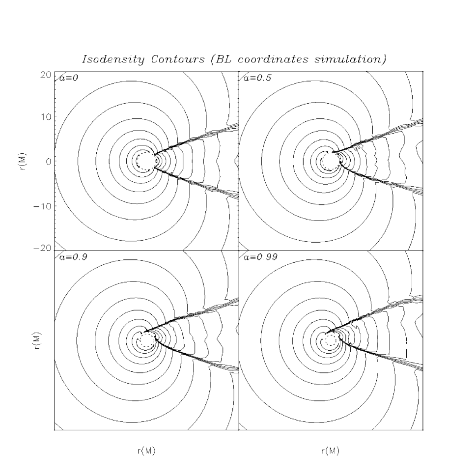
Figure 1: Flow morphology at a final time $t=500M$. We plot 20 isocontours of the logarithm of the density (scaled to its asymptotic value) for the first four models considered in Table 1 ($a=0,0.5,0.9$ and $0.99$, in units of the mass of the black hole). The presence of a well-defined tail shock is clearly noticeable in all cases. The minimum value of $\log\rho$ for all models is $-0.26$ whereas the maximum, always found in the rear (right) part of the black hole, increases with $a$: $1.65$, $1.69$, $1.75$ and $1.77$ for models 1 to 4, respectively. The domain of the plot extends up to $20M$. Asymptotically the flow moves from left to right. By the final time of $500M$ the flow pattern is already stationary. This figure corresponds to a simulation performed with Boyer-Lindquist coordinates. The innermost dashed line indicates the position of the black hole horizon.

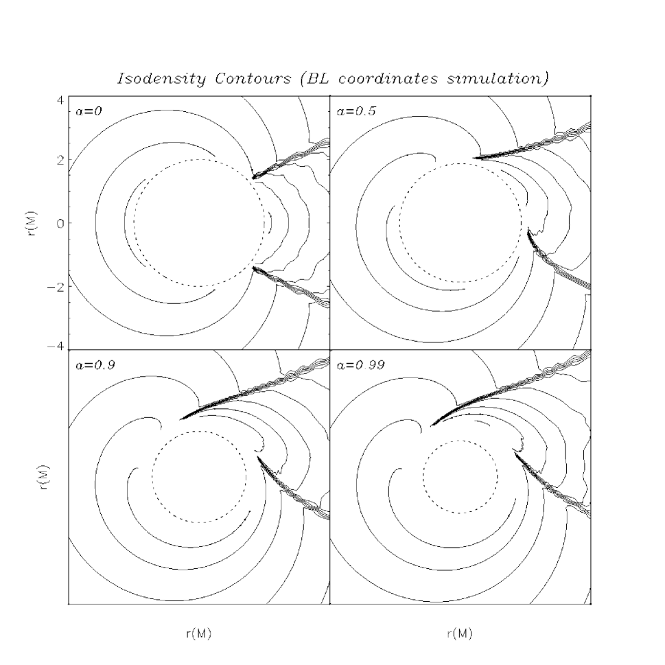
Figure 2: This figure represents a zoomed view of Fig. 1. Now the domain of the plot extends up to $4M$. The effects of the rotation of the black hole on the flow morphology become increasingly evident in the regions closer to the black hole horizon. Its location is indicated by the dashed line. Note that the inner radius of the computational domain is, in BL coordinates, clearly separated from $r_{+}$, specially for rapidly-rotating holes.

In Fig. 1 we display the flow pattern for the first four models of Table 1, which corresponds to a final time of $500M$. This is a Cartesian plot where the $x$ and $y$ axis are, respectively, $r\cos{\phi}$ and $r\sin{\phi}$. We plot isocontours of the logarithm of the rest-mass density, properly scaled by its asymptotic value. These results are obtained employing BL coordinates. The outer domain of this figure corresponds to $20M$. Similarly, in Fig. 2 we plot a close-up view of that domain, up to a distance of $4M$. The dotted innermost line, in both figures, represents the location of the horizon $r_{+}$.

All models are characterized by the presence of a well-defined tail shock. As already shown in FI98b, in non-axisymmetric relativistic Bondi-Hoyle accretion simulations, this shock appears stable to tangential oscillations, in contrast to Newtonian simulations with tiny accretors (see, e.g., Benensohn et al 1997 and references there in). By direct inspection of these figures, the effect of the rotation of the black hole on the flow morphology becomes clear. The shock becomes wrapped around the central accretor as the black hole angular momentum $a$ increases. The effect is, though, localized to the central regions. In the $a=0.5$ plot we see that the morphology of the shock deviates from the pattern of the non-rotating case inside approximately $r=4M$. For $a=0.9$, the region of influence extends slightly further out, to about $r=5M$. At the outer regions, as expected, the overall morphology is remarkably similar for all values of $a$. This is not surprising, since the Kerr metric rapidly approaches the Schwarzschild form for radii large compared to $r_{+}$. This fact, in turn, shows that possible telltale signals of a rotating black hole,in an astrophysical context, demand an accurate description of the innermost regions.

In Figs. 3 and 4 we show the final configuration for the density for the same initial setups as in Figs. 1 and 2, but now for simulations employing the KS coordinate system. We construct the plots using the standard transformation between KS and Cartesian coordinates $x+iy=(r+ia)\sin\theta e^{i\tilde{\phi}}$ (Hawking and Ellis 1972) with $\theta=\pi/2$ . Again, the dotted line in these plots indicates the position of $r_{+}$. Notice that in KS coordinates the computation extends inside the horizon (this is more clearly seen in Fig. 4). The flow morphology shows smooth behaviour when crossing the horizon, all matter fields being regular there. We observe here the same confinement of rotational effects to the innermost regions around the black hole. Notably though, the shock structure appears less deformed, especially the lower component. The reason is that in the BL description of the black hole geometry, the dominant effects near the horizon are purely kinematic (associated with coordinate system pathologies) and dissapear with the adoption of a regular system. Clearly, the accurate description of near horizon effects can be achieved easier when using horizon adapted coordinate systems.

As in the non-rotating studies (FI98a,b), we also notice that the most efficient region of the accretion process is the rear part of the black hole. The material flowing inside some radius smaller than the characteristic impact parameter of the problem (say, the accretion radius, see below) after changing its sense of motion due to the strong gravitational field is acummulated behind the black hole and is gradually accreted. We find that this maximum density always increases with $a$ and its functional dependence is clearly greater than linear. The specific values we obtain can be found in the corresponding captions of Figs. 1 to 4. Typical density enhancements in the post-shock region (BL coordinates) with respect to the asymptotic density range in between $1.65$ ($a=0$) and $1.77$ ($a=0.99$) (in logarithmic scale).

Now we turn to the description of the flow morphology for different values of $\gamma$, the fluid adiabatic exponent. The accretion patterns for models 6 ($\gamma=4/3$), 4 ($\gamma=5/3$) and 7 ($\gamma=2$) are depicted in Fig. 5. Once more, the variable we show in this figure is the logarithm of the scaled rest-mass density. Clearly visible in this plot are the larger shock opening angles for the larger values of $\gamma$. This is explained by the enhanced values of the pressure inside the shock “cone” as $\gamma$ increases. We already noticed this behaviour in the non-rotating simulations performed in FI98a,b. Now, the larger values of $\gamma$, combined with the rapid rotation of the black hole ($a=0.99$), wrap the upper shock wave around the accretor. This effect is more pronounced for the larger $\gamma$ values. We also note that the lower shock wave is less affected by the increase in $\gamma$. While it still opens to larger angles, the existing rotational flow counteracts the effects of the pressure force keeping its position almost unchanged.

The enhancement of the pressure in the post-shock zone is responsible for the so-called “drag” force experienced by the accretor. We notice here that the rotating black hole is redistributing the high pressure area, with non-trivial effects on the nature of the drag force. Whereas in the Schwarzschild case the drag force is alligned with the flow lines, pointing in the upstream direction, in the Kerr case we notice a distinct asymmetry between the co-rotating and counter-rotating side of the flow. The pressure enhancement is predominantly on the counter-rotating side. In Fig. 6 this observation is made more precise with the examination of the pressure profile, at the innermost radius, for the $a=0.99$ case. Three different $\gamma$ values are illustrated, showing the strong dependence of the pressure asymmetry on the adiabatic index. This is particularly clear in the limiting case $\gamma=2$ (dashed line). We observe a pressure difference of almost two orders of magnitude, along the axis normal to the asymptotic flow direction. The implication of this asymmetry is that a rotating hole moving accross the interstellar medium (or accreting from a wind), will experience, on top of the drag force, a “lift” force, normal to its direction of motion (to the wind direction).

It is interesting to note that this effect bears a strong superficial resemblance to the so-called “Magnus” effect, i.e., the experience of lift forces by rotating bodies immersed in a stream flow. There, the lift force is due to the increased speed of the flow on the co-rotating side (due to friction with the object), and the increase of pressure on the counter-rotating side (which follows immediately from the Bernoulli equation). We note that the direction of the lift, in relation to the sense of rotation, agrees in both contexts. We caution though that the underlying causes may be very different. In the black hole case the flow is supersonic and there is no boundary layer.

Completing the study of the broad morphology of the flow and its dependence on the black hole spin, we extend the value of $a$ above $M$, choosing, in particular, $a=1.1M$ (model 5). This case corresponds to accretion onto a naked singularity. Although from the theoretical point of view such objects are believed not to exist in Nature (according to the Cosmic Censorship hypothesis, all physical singularities formed by the gravitational collapse of nonsingular, asymptotically flat initial data, must be hidden from the exterior world inside an event horizon) we nonetheless decided to perform such a computation, in order to assess the behaviour of the code in this regime, and to explore the extrapolation of previous simulations. The resulting morphology for this simulation, using KS coordinates, is plotted in Fig. 7. We are showing isocontours of the logarithm of the rest-mass density in a region extending $4M$ in the $x$ and $y$ directions from the singularity. In this situation, there is an ambiguity as to where to place the inner boundary of the domain. The closer one gets to $r=0$ the stronger the gravity becomes (with infinite tidal forces at the singularity). This introduces important resolution requirements on the numerical code. For this reason we chose $r_{min}=M$, in accordance with the location of the inner boundary in the maximal case $a=M$. As can be seen from Fig. 7 the flow morphology for this model follows the previous trend found for lower values of $a$ (models 1 to 4): the shock appears slightly more wrapped (around the $r=M$ circle) and the maximum rest-mass density in the rear part of the accretor increases.

3.3 Accretion rates

We compute the accretion rates of mass, radial momentum and angular momentum. The procedure of computation can be found in FI98a and FI98b. The rates are typically evaluated at the accretion radius, $r_{a}$, defined as

$$r_{a}=\frac{M}{v_{\infty}^{2}+c_{s_{\infty}}^{2}}.$$ (44)

For our models $r_{a}=3.85M$. The results are plotted in Figs. 8-10 for BL coordinates and in Figs. 11-13 for the KS system. In these figures we show the time evolution of those rates for the whole simulation. For comparison purposes, the radial and angular momentum accretion rates have been scaled to one (scaling by a factor of 1250 and 80, respectively in the BL coordinate runs; correspondingly, with KS coordinates these factors are 300 and 400). We have checked that, as expected, the qualitative behavior of the accretion rates is independent of the radius at which they are computed, as long as a stationary solution is found.

All rates show a clear transition to a final stationary state, around the time interval $100M-200M$, regardless of the coordinate system used. The non-rotating case ($a=0$) shows no signs of oscillations, leading to remarkably constant values for all rates (again independent of the coordinates). Non zero $a$ values are seen to show considerable more oscillatory behavior around some average value. The reason behind this effect is purely numerical. The black hole geometry leads, in the rotating case, to a significantly larger number of non-zero Christoffel symbols, which appear explicitly in the source terms of the hydrodynamic equations (see the Appendix). Increasing the resolution (in particular the angular one), considerably reduces the amplitude of the oscillations, as can be read off Fig. 14.

The mass accretion rates have been scaled to the canonical value proposed by Petrich et al (1989). In KS coordinates (Fig. 11) this value is larger than in BL coordinates (Fig. 8). However, this is just a coordinate effect as we show in the next section. In addition, in Fig. 8 there appears to be a certain trend on the variation of the mass rate with $a$, being (slightly) larger for larger values of $a$. This is not the case for KS coordinates, where the normalized mass accretion rate is around $156$, regardless of the value of $a$. We will come back to this issue later in this section.

In Fig. 9 we plot the (scaled) radial momentum accretion rate for BL coordinates. The maximum drag rate is obtained for non-rotating holes. As for the mass accretion rate, the radial momentum rate also shows a clear dependence on $a$, especially when using BL coordinates. This dependence is not so clear for KS coordinates (see Fig. 12). This discrepancy will be explained below. Note also that due to the different scale factors used, the radial momentum rates in Fig. 9 are a factor 4 larger than those of Fig. 12.

Finally, the angular momentum accretion rates (Figs. 10 and 13) are clearly non-zero for rotating black holes in contrast to the $a=0$ case. For both coordinate systems it exhibits a clear trend: the larger the value of $a$ the larger the angular momentum rate. Due to the different scales used in the different coordinates, the angular momentum rates in Fig. 10 are a factor 5 smaller than those in Fig. 13.

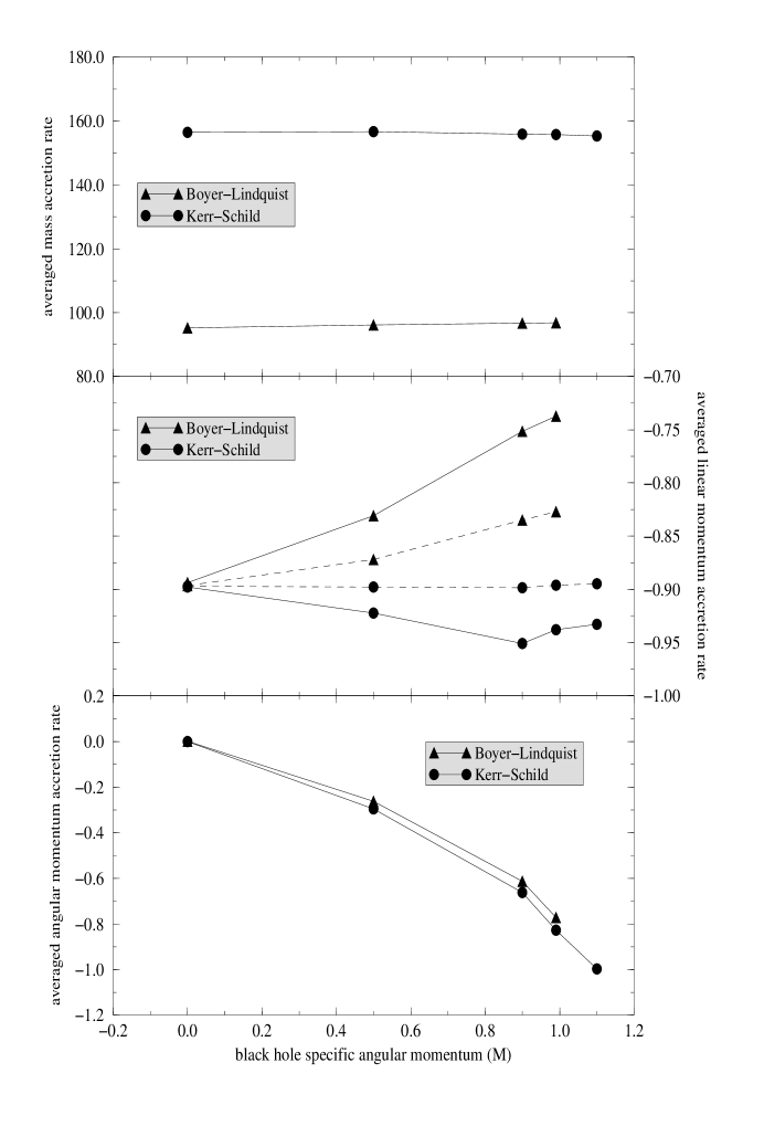
Figure 15: Averaged accretion rates of mass (top), linear momentum (middle) and angular momentum (bottom) versus the black hole spin. All rates are averaged at the final $200M$ of the evolution. They are all computed at the accretion radius except for the linear momentum rate which is also computed at $r_{max}$ (dashed lines). The non-dependence of the mass and linear momentum rates with $a$ is noticeable, especially for the KS coordinate system. For the linear momentum rate this is particularly true when computed at large radii ($r_{max}$, dashed lines) but does not hold, for numerical reasons, at small radii ($r_{a}$, solid lines).

To clarify the discrepancies found in the computation of the accretion rates in the different coordinate systems we plot in Fig. 15 the dependence of those rates with the specific angular momentum of the black hole. In order to do so, we average the rates over the final $200M$ of the evolution, once the steady state is well established. Results for the BL system are depicted with a filled triangle whereas results for the KS system are represented by filled circles. We are only considering the subset of models 1-5 in Table 1. As in the previous figures, the momentum accretion rates have been properly scaled with adequate factors. The radial momentum rates presented in this plot are computed both at $r_{a}$ (solid lines) and at $r_{max}$ (dashed lines). From this figure the non-dependence of the mass accretion rate on $a$ becomes more clear. This is the expected result, as the mass accretion rate is an integral invariant, and hence does not change by deformations of the surface over which it is computed. Deforming this surface outwards, by increasing the radius at which the mass accretion rate is measured, must lead to the same result, so long as the solution is in a steady state. At sufficiently large radii, the rotating aspect of the metric is essentially “hidden” and the accretion rate should depend only on the total mass of the central potential. We conclude that the larger discrepancies found when computing the mass accretion rate in the BL coordinates (see Fig. 7 for models 1 to 4) are purely due to numerical reasons, induced for instance, by the more extreme dynamical behaviour of some fields in the near zone of the black hole potential. However, the deviations never exceed a few percent, more specifically, $1.5\%$ for the BL system simulation and $1.2\%$ using KS coordinates.

Coming back to the radial momentum accretion rate computation, we have verified that its dependence on the black hole angular momentum is strongly related to the radius at which it is computed. We find that at large radii its value remains remarkably constant for all values of $a$. In Figs. 9 and 12 we plot the drag rate computed at the accretion radius. In BL coordinates (Fig. 9) we get a $15\%$ difference between the $a=0$ and $a=0.99$ cases. For KS coordinates (Fig. 12) this difference is reduced to $5\%$. However, if the radial momentum accretion rate is computed at $r_{max}$ (as in Fig. 15, dashed lines) we obtain significantly smaller differences: $7\%$ for BL coordinates and only $0.4\%$ for KS coordinates.

We quantify next how the mass accretion rate depends on the arbitrary location (but necessarily larger than $r_{+}$) of the inner boundary in BL coordinates. Placing this inner boundary at $r=2.1M$ for model 3 we find the surprising result that, although the broad flow morphology looks qualitatively similar in both cases, the accretion rates strongly depend on the value of the innermost radius. We note that a small change in location (such as from $1.89M$ to $2.1M$) introduces, roughly, a $10\%$ difference on the computed mass accretion rate.

Fig. 15 also illustrates the dependence of the angular momentum accretion rate with the spin of the black hole. Clearly, this quantity increases with $a$ in a non-linear way.

We complete our study of the different accretion rates presenting their dependence on the fluid adiabatic index. To do this, we choose the rapidly rotating hole ($a=0.99M$) of models 4, 6 and 7. Table 2 shows the results obtained using the KS coordinate system. Again, we are averaging the accretion rates on the final $200M$ of evolution. We note that we are now choosing a different normalization. The reason is that the canonical mass accretion rate we are using to scale all rates (see Petrich et al 1989; see also Shapiro and Teukolsky 1983) is ill defined for $\gamma>5/3$. As we are mostly interested in their qualitative behaviour and not in the particular numbers, re-normalizing all rates to unity suffices for our purposes. Our numerical study shows that all accretion rates decrease (in absolute value for the momentum rates) as $\gamma$ increases from $4/3$ to $2$. This is in contrast with the results presented in FI98a for the non-rotating case. However, this is just an apparent disagreement related to the different normalization procedures employed in the two surveys.

3.4 Coordinate system comparison

We focus now on a direct comparison between the accretion patterns obtained with the different coordinate systems. In order to do so we take advantage of the stationarity of the solution at late times. In Fig. 16 we show the setup that allows for a simple comparison between the BL and KS coordinate systems in the case of stationary flows. For such flows, a one-to-one correspondence between physical points can be established using the appropriate coordinate transformations presented before.

The procedure of comparison involves a transformation from $(r,\tilde{\phi})$ coordinates to $(r,\phi)$ and, finally, to $(x,y)\equiv(r\cos\phi,r\sin\phi)$. For the case of scalar quantities, such as the density, the comparison procedure ends here. For vector fields, such as the velocity, we employ in addition the linear transformations given by Eqs. (26)-(28).

We focus on model 4 of Table 1 ($a=0.99M$). Fig. 17 shows the isodensity contours at the final time ($t=500M$) in BL coordinates. The left panel corresponds to an actual BL evolution, while the right one shows how results from a simulation originally performed in KS coordinates look like when transformed to BL coordinates. The innermost dotted circle marks the location of the horizon. The dashed line marks the position of $r_{min}$ in BL coordinates (we intentionally cut out the interior region in the right panel). The qualitative agreement of the two plots is remarkable.

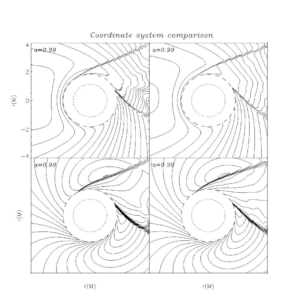
Figure 18: Comparison of the stationary accretion pattern (model 4). Isocontours of the radial (top) and azimuthal (bottom) 3-velocity components. The left and right panels follow the same convention of Fig. 17. The agreement in the simulations is again excellent.

We turn now to the comparison of the radial and azimuthal components of the velocity. This is depicted in Fig. 18. The convention for the left and right panels follows the same criteria as in Fig. 17. Again, the agreement is excellent, even though comparing these two quantities involves, besides the coordinate shift (from $\tilde{\phi}$ to $\phi$), also a non-trivial linear transformation.

From these figures one can notice that the smooth features of the solution (i.e., the pre-shocked part of the flow) are well captured in both systems, whereas the shock and the innermost regions present slightly more numerical noise in BL coordinates. Notice also that, although in BL coordinates we are forced to cut out an important domain of integration (due to numerical instabilities associated to this pathological system), it is also true that the solution does not seem to be qualititavely affected, at least for the flows considered here. This may be explained by the fact that the flow is highly supersonic at the innermost zone. This simplifies the task of imposing appropriate boundary conditions there, e.g., a simple linear extrapolation will always work.

It is instructive to see how the solution would look like in BL coordinates if the location of $r_{min}$ were moved inwards. This is plotted in Fig. 19. Here we show isodensity contours starting in a region much closer to the horizon than in Fig. 17 (note that at the horizon the coordinate transformation is singular). We can now follow the shock location all the way down to those inner regions, showing the singular spiralling around the central hole.

As our final comparison between quantities computed in the two coordinate systems we study the correlation of the mass accretion rates. In order to do so, we must compute the mass rate with respect to proper time, through a given physical surface. The relation between the proper, $\tau$, and coordinate, $t$, times (which is the one employed in the plots of the accretion rates) involves the lapse function, $d\tau=\alpha dt$. Making the comparison, hence, requires including the ratio of the lapse in the two coordinate systems at that physical location. The final relation is given by the surface integral

$${\dot{m}}_{BL}=-\int\frac{1}{\Psi}D\alpha\sqrt{\gamma}\left(v^{\tilde{r}}-\frac{\beta^{\tilde{r}}}{\alpha}\right)d\Sigma$$ (45)

where ${\dot{m}}$ denotes the rate of change in (coordinate) time of the mass accreted and all quantities (except $\Psi$, see Eq. (30)) in the integrand are computed in the KS system. The result of the comparison, for model 4, is plotted in Fig. 20. We show the mass accretion rate sampled at discrete (coordinate) times (every $50M$). The circles indicate the mass accretion estimate in the original BL simulation. The plus signs show this rate as a result of the transformation from the KS simulation. We can again conclude that the qualitative agreement is good, especially, and as expected by the comparison procedure we use, once the steady-state is reached.

4 Discussion

In this paper we have presented detailed numerical computations of non-axisymmetric relativistic Bondi-Hoyle accretion onto a rotating (Kerr) black hole. The integrations have been performed with an advanced high-resolution shock-capturing scheme based on an approximate Riemann solver. In particular, we have studied accretion flows onto rapidly-rotating black holes.

We have demonstrated that even in the presence of rotation, the relativistic accretion patterns always proceed in a stationary way. This seems to be a common feature of relativistic flows as opposed to non-axisymmetric Newtonian computations. Previous relativistic simulations for Schwarzschild (non-rotating) black holes already pointed out this stability (FI98b). The physical minimum size of the accretor considered now is $r_{+}=M$, the (outermost) event horizon of a Kerr black hole. For our initial data, the minimum value corresponds to $0.29r_{a}$, with $r_{a}$ being the accretion radius. This parameter controls the appearance of the tangential instability in Newtonian flows. The instability was found there to appear only for tiny accretors. Although we have now smaller accretors than in the Schwarzschild case the flow patterns still relax to a final steady-state.

The effects of the black hole rotation on the flow morphology were seen to be confined to the inner regions of the black hole potential. Within this region, the black hole angular momentum drags the flow, wrapping the shock structure around, and generating an overpressure on the counter-rotating side. This is reminiscent of similar behavior in classical fluid mechanics (i.e., the Magnus effect), although there does not appear to be a deeper physical similarity between the two contexts.

As a hypothetical scenario, we have also considered accretion flows onto a naked singularity ($a>M$). Our preliminary observation is that the morphology of the flow in this case is a smooth continuation of the black hole simulations.

The validity of the results has been double-checked by performing the simulations in two different coordinate systems. A gratifying result of our study, confirming the accuracy of the computations, is the overall agreement obtained in this comparison (performed for a variety of matter fields), taking advantage of the stationarity of the final accretion flow. Although the transformations of scalars and vectors from one coordinate system to the other are far from trivial, we have found good overall agreement in our results.

The stationarity of the solution has been also demonstrated computing the accretion rates of mass and momentum. Those rates were found to depend on the coordinate system used, but they roughly agree when transformed to the same frame. The mass and radial momentum rates show (slight) dependence on the spin of the black hole when using BL coordinates, but not so for the KS system. As those quantities should be independent of the black hole angular momentum, the computations using KS coordinates were, numerically, more accurate. On the other hand, as one would expect, the angular momentum accretion rates vanish only for Schwarzschild holes and substantially increase as $a$ increases. We have also presented the dependence of the different accretion rates on the adiabatic index of the (perfect fluid) equation of state. The results found for a rotating black hole with $a=0.99M$ show smaller values for all rates as $\gamma$ increases.

We have shown that the choice of the Kerr-Schild form of the Kerr metric, regular at the horizon, allows for more accurate integrations of the general relativistic hydrodynamic equations than the standard singular choice (i.e., Boyer-Lindquist coordinates). Such horizon adapted (regular) systems eliminate numerical inconsistencies by placing the inner boundary of the domain inside the black hole horizon, hence, causally disconnecting unwanted boundary influences.

Appendix

In this appendix we write down, explicitly, the fluxes and the source terms of the general relativistic hydrodynamic equations for the Kerr line element. In addition, we also write the non-vanishing Christoffel symbols needed for the computation of the sources. All the expressions are written for the two different system of coordinates used in the computations and are specialized for the equatorial plane $(\theta=\pi/2)$.

Fluxes

Boyer-Lindquist:

$${\bf F}^{r}({\bf w})=\left(Dv^{r},S_{r}v^{r}+p,S_{\phi}v^{r},(\tau+p)v^{r}\right)$$ (46)

$${\bf F}^{\phi}({\bf w})=\left(D\left(v^{\phi}-{{\beta^{\phi}}\over{\alpha}}\right),S_{r}\left(v^{\phi}-{{\beta^{\phi}}\over{\alpha}}\right),S_{\phi}\left(v^{\phi}-{{\beta^{\phi}}\over{\alpha}}\right)+p,\tau\left(v^{\phi}-{{\beta^{\phi}}\over{\alpha}}\right)+pv^{\phi}\right).$$ (47)

Kerr-Schild:

$${\bf F}^{r}({\bf w})=\left(D\left(v^{r}-\frac{\beta^{r}}{\alpha}\right),S_{r}\left(v^{r}-\frac{\beta^{r}}{\alpha}\right)+p,S_{\tilde{\phi}}\left(v^{r}-\frac{\beta^{r}}{\alpha}\right),\tau\left(v^{r}-\frac{\beta^{r}}{\alpha}\right)+pv^{r}\right)$$ (48)

$${\bf F}^{\tilde{\phi}}({\bf w})=\left(Dv^{\tilde{\phi}},S_{r}v^{\tilde{\phi}},S_{\tilde{\phi}}v^{\tilde{\phi}}+p,(\tau+p)v^{\tilde{\phi}}\right)$$ (49)

Sources

$${\bf S}({\bf w})=(S_{1},S_{2},S_{3},S_{4})$$ (50)

Boyer-Lindquist:

$$S_{1} = -\alpha Dv^{r}\Omega$$ (51)

$$S_{2} = -\alpha(S_{r}v^{r}+p)\Omega+\alpha T^{rr}g_{rr,r}-\alpha A_{1}g_{rr}$$ (52)

$$S_{3} = -\alpha S_{\phi}v^{r}\Omega+\alpha T^{rt}g_{t\phi,r}+\alpha T^{r\phi}g_{\phi\phi,r}-2\alpha A_{2}g_{t\phi}-2\alpha A_{3}g_{\phi\phi}$$ (53)

$$S_{4} = -\alpha(\tau+p)v^{r}\Omega+\alpha T^{tr}\alpha_{,r}-2\alpha^{2}A_{2}$$ (54)

with the definitions

$$\Omega = {{1}\over{r}}+{{\Sigma_{,r}}\over{2\Sigma}}-{{\Delta_{,r}}\over{2\Delta}}$$ (55)

$$A_{1} = T^{tt}\Gamma^{r}_{tt}+T^{rr}\Gamma^{r}_{rr}+T^{\theta\theta}\Gamma^{r}_{\theta\theta}+T^{\phi\phi}\Gamma^{r}_{\phi\phi}+2T^{t\phi}\Gamma^{r}_{t\phi}$$ (56)

$$A_{2} = T^{r\phi}\Gamma^{t}_{r\phi}+T^{tr}\Gamma^{t}_{tr}$$ (57)

$$A_{3} = T^{r\phi}\Gamma^{\phi}_{r\phi}+T^{tr}\Gamma^{\phi}_{tr}$$ (58)

with $T^{\mu\nu}$ being the perfect fluid stress-energy tensor

$$T^{\mu\nu} = \rho hu^{\mu}u^{\nu}+pg^{\mu\nu}.$$ (59)

The ‘,’ denotes partial differentiation and the $\Gamma^{\delta}_{\mu\nu}$ stand for the Christoffel symbols. Quantity $h$ appearing in the stress-energy tensor is the specific enthalpy, $h=1+\varepsilon+p/\rho$.

Kerr-Schild:

$$S_{1} = -\alpha D\left(v^{r}-\frac{\beta^{r}}{\alpha}\right)\Theta$$ (60)

$$S_{2} = -\alpha\left(S_{r}\left(v^{r}-\frac{\beta^{r}}{\alpha}\right)+p\right)\Theta+$$ (61)

$$\alpha\left[T^{{\tilde{t}}r}g_{{\tilde{t}}r,r}+T^{rr}g_{rr,r}+T^{r{\tilde{\phi}}}g_{r{\tilde{\phi}},r}-\right.\left.\beta_{r}B_{1}-g_{rr}B_{2}-g_{r{\tilde{\phi}}}B_{3}\right]$$

$$S_{3} = -\alpha\left(S_{{\tilde{\phi}}}\left(v^{r}-\frac{\beta^{r}}{\alpha}\right)\right)\Theta+$$ (62)

$$\alpha\left[T^{{\tilde{t}}r}g_{{\tilde{t}}{\tilde{\phi}},r}+T^{rr}g_{r{\tilde{\phi}},r}+T^{r{\tilde{\phi}}}g_{{\tilde{\phi}}{\tilde{\phi}},r}-\right.\left.\beta_{\tilde{\phi}}B_{1}-g_{r{\tilde{\phi}}}B_{2}-g_{{\tilde{\phi}}{\tilde{\phi}}}B_{3}\right]$$

$$S_{4} = -\alpha\left(\tau\left(v^{r}-\frac{\beta^{r}}{\alpha}\right)+pv^{r}\right)\Theta+\alpha T^{{\tilde{t}}r}\alpha_{,r}-\alpha^{2}B_{1}$$ (63)

with

$$\Theta = \frac{2r-M\alpha^{2}}{r^{2}}$$ (64)

$$B_{1} = T^{{\tilde{t}}{\tilde{t}}}\Gamma^{{\tilde{t}}}_{{\tilde{t}}{\tilde{t}}}+T^{rr}\Gamma^{{\tilde{t}}}_{rr}+T^{\theta\theta}\Gamma^{{\tilde{t}}}_{\theta\theta}+T^{{\tilde{\phi}}{\tilde{\phi}}}\Gamma^{{\tilde{t}}}_{{\tilde{\phi}}{\tilde{\phi}}}+2(T^{{\tilde{t}}r}\Gamma^{{\tilde{t}}}_{{\tilde{t}}r}+T^{{\tilde{t}}{\tilde{\phi}}}\Gamma^{{\tilde{t}}}_{{\tilde{t}}{\tilde{\phi}}}+T^{r{\tilde{\phi}}}\Gamma^{{\tilde{t}}}_{r{\tilde{\phi}}})$$ (65)

$$B_{2} = T^{{\tilde{t}}{\tilde{t}}}\Gamma^{r}_{{\tilde{t}}{\tilde{t}}}+T^{rr}\Gamma^{r}_{rr}+T^{\theta\theta}\Gamma^{r}_{\theta\theta}+T^{{\tilde{\phi}}{\tilde{\phi}}}\Gamma^{r}_{{\tilde{\phi}}{\tilde{\phi}}}+2(T^{{\tilde{t}}r}\Gamma^{r}_{{\tilde{t}}r}+T^{{\tilde{t}}{\tilde{\phi}}}\Gamma^{r}_{{\tilde{t}}{\tilde{\phi}}}+T^{r{\tilde{\phi}}}\Gamma^{r}_{r{\tilde{\phi}}})$$ (66)

$$B_{3} = T^{{\tilde{t}}{\tilde{t}}}\Gamma^{{\tilde{\phi}}}_{{\tilde{t}}{\tilde{t}}}+T^{rr}\Gamma^{{\tilde{\phi}}}_{rr}+T^{\theta\theta}\Gamma^{{\tilde{\phi}}}_{\theta\theta}+T^{{\tilde{\phi}}{\tilde{\phi}}}\Gamma^{{\tilde{\phi}}}_{{\tilde{\phi}}{\tilde{\phi}}}+2(T^{{\tilde{t}}r}\Gamma^{{\tilde{\phi}}}_{{\tilde{t}}r}+T^{{\tilde{t}}{\tilde{\phi}}}\Gamma^{{\tilde{\phi}}}_{{\tilde{t}}{\tilde{\phi}}}+T^{r{\tilde{\phi}}}\Gamma^{{\tilde{\phi}}}_{r{\tilde{\phi}}})$$ (67)

Non-vanishing Christoffel symbols

Boyer-Lindquist:

$$\Gamma^{t}_{tr} = {{M}\over{\Delta r^{2}}}(a^{2}+r^{2})$$ (68)

$$\Gamma^{t}_{r\phi} = -{{aM}\over{\Delta r^{2}}}(a^{2}+3r^{2})$$ (69)

$$\Gamma^{r}_{tt} = -{{\Delta M}\over{r^{4}}}$$ (70)

$$\Gamma^{r}_{rr} = {{1}\over{r\Delta}}(a^{2}-Mr)$$ (71)

$$\Gamma^{r}_{\theta\theta} = -{{\Delta}\over{r}}$$ (72)

$$\Gamma^{r}_{\phi\phi} = {{\Delta}\over{r^{4}}}(Ma^{2}-r^{3})$$ (73)

$$\Gamma^{r}_{t\phi} = -{{Ma\Delta}\over{r^{4}}}$$ (74)

$$\Gamma^{\phi}_{r\phi} = -{{1}\over{\Delta r^{2}}}(Ma^{2}+r^{2}(2M-r))$$ (75)

$$\Gamma^{\phi}_{tr} = {{Ma}\over{\Delta r^{2}}}$$ (76)

Kerr-Schild:

$$\Gamma^{\tilde{t}}_{\tilde{t}\tilde{t}} = \frac{2M^{2}}{r^{3}}$$ (77)

$$\Gamma^{\tilde{t}}_{\tilde{t}r} = \frac{M(r+2M)}{r^{3}}$$ (78)

$$\Gamma^{\tilde{t}}_{\tilde{t}\tilde{\phi}} = -\frac{2M^{2}a}{r^{3}}$$ (79)

$$\Gamma^{\tilde{t}}_{rr} = \frac{2M(M+r)}{r^{3}}$$ (80)

$$\Gamma^{\tilde{t}}_{r\tilde{\phi}} = -\frac{Ma(r+2M)}{r^{3}}$$ (81)

$$\Gamma^{\tilde{t}}_{\theta\theta} = -2M$$ (82)

$$\Gamma^{\tilde{t}}_{\tilde{\phi}\tilde{\phi}} = \frac{2M(Ma^{2}-r^{3})}{r^{3}}$$ (83)

$$\Gamma^{r}_{\tilde{t}\tilde{t}} = \frac{M\Delta}{r^{4}}$$ (84)

$$\Gamma^{r}_{\tilde{t}r} = -\frac{M(2Mr-a^{2})}{r^{4}}$$ (85)

$$\Gamma^{r}_{\tilde{t}\tilde{\phi}} = -\frac{Ma\Delta}{r^{4}}$$ (86)

$$\Gamma^{r}_{rr} = -\frac{M(2Mr+r^{2}-a^{2})}{r^{4}}$$ (87)

$$\Gamma^{r}_{r\tilde{\phi}} = \frac{a(2M^{2}r+r^{3}-Ma^{2})}{r^{4}}$$ (88)

$$\Gamma^{r}_{\theta\theta} = -\frac{\Delta}{r}$$ (89)

$$\Gamma^{r}_{\tilde{\phi}\tilde{\phi}} = -\frac{r^{5}-2Mr^{4}+a^{2}r^{3}-Ma^{2}r^{2}+2M^{2}a^{2}r-Ma^{4}}{r^{4}}$$ (90)

$$\Gamma^{\theta}_{r\theta} = \frac{1}{r}$$ (91)

$$\Gamma^{\tilde{\phi}}_{\tilde{t}\tilde{t}} = \frac{Ma}{r^{4}}$$ (92)

$$\Gamma^{\tilde{\phi}}_{\tilde{t}r} = \frac{Ma}{r^{4}}$$ (93)

$$\Gamma^{\tilde{\phi}}_{\tilde{t}\tilde{\phi}} = -\frac{Ma}{r^{4}}$$ (94)

$$\Gamma^{\tilde{\phi}}_{rr} = \frac{Ma}{r^{4}}$$ (95)

$$\Gamma^{\tilde{\phi}}_{r\tilde{\phi}} = -\frac{Ma^{2}-r^{3}}{r^{4}}$$ (96)

$$\Gamma^{\tilde{\phi}}_{\theta\theta} = -\frac{a}{r}$$ (97)

$$\Gamma^{\tilde{\phi}}_{\tilde{\phi}\tilde{\phi}} = \frac{a(Ma^{2}-r^{3})}{r^{4}}$$ (98)

Table 1
Initial models
MODEL	$\gamma$	${\cal M}_{\infty}$	$v_{\infty}$	$a$	$r_{+}$	$r_{min}$ (BL)	$r_{max}$ (BL)	$r_{min}$ (KS)	$r_{max}$ (KS)
1	$5/3$	$5.0$	$0.5$	$0$	$2$	$2.2$	$38.5$	$1.8$	$50.9$
2	$5/3$	$5.0$	$0.5$	$0.5$	$1.87$	$2.08$	$34.7$	$1.8$	$50.9$
3	$5/3$	$5.0$	$0.5$	$0.9$	$1.44$	$1.89$	$34.9$	$1.4$	$50.9$
4	$5/3$	$5.0$	$0.5$	$0.99$	$1.14$	$1.83$	$35.0$	$1.14$	$50.9$
5	$5/3$	$5.0$	$0.5$	$1.1$	$-$	$-$	$-$	$1.0$	$50.9$
6	$4/3$	$5.0$	$0.5$	$0.99$	$1.14$	$-$	$-$	$1.0$	$50.9$
7	$2$	$5.0$	$0.5$	$0.99$	$1.14$	$-$	$-$	$1.0$	$50.9$

Table 1.- $\gamma$ is the adiabatic exponent of the fluid, ${\cal M}_{\infty}$ is the asymptotic Mach number, $v_{\infty}$ is the asymptotic flow velocity, $a$ is the Kerr angular momentum parameter, $r_{+}$ indicates the location of the horizon and $r_{min}$ and $r_{max}$ are the minimum and maximum radial values of the computational domain. BL stands for Boyer-Lindquist and KS for Kerr-Schild. All distances are measured in units of the mass of the hole, which we chose equal to 1. Note that model 5 represents a “naked” singularity $(a>1)$.

Table 2
Accretion rates versus fluid adiabatic index
MODEL	$\gamma$	mass	linear momentum	angular momentum
4	$4/3$	$0.94$	$-0.98$	$-0.91$
4	$5/3$	$0.83$	$-0.98$	$-0.69$
4	$2$	$0.74$	$-0.85$	$-0.67$

Table 2.- Dependence of the different accretion rates on the adiabatic index of the fluid for model 4 ($a=0.99M$). The results are for KS coordinates. All rates are averaged on the final $200M$ of the simulation and conveniently scaled to one.

Figure 3: Flow morphology at $t=500M$ for a simulation using Kerr-Schild coordinates. As in Fig. 1 we plot 20 isocontours of the logarithm of the scaled rest-mass density for the first four models of Table 1. The minimum value of $\log\rho$ for all models is now $-0.16$. The maximum, again, increases with $a$: $1.96$, $1.97$, $2.13$ and $2.27$ for models 1 to 4, respectively. The domain of the plot extends up to $20M$. The horizon of the black hole is now included in the computational domain. The shock extends all the way to the horizon, $r_{+}$, which is indicated by the innermost dashed line.

Figure 4: This figure represents a zoomed view of Fig. 3. Now the domain of the plot extends up to $4M$. As in Fig. 2, the effects of the angular momentum of the black hole on the accreting matter are more noticeable at the black hole close vicinity. The horizon is again represented by the innermost dashed line. Contrary to the BL evolutions, the inner radius of the domain includes now the black hole horizon. Notice that the presence of the horizon is totally “transparent” to the matter flow.

Figure 5: Stationary flow morphology for three different values of $\gamma$, the fluid adiabatic index: $4/3$ (top), $5/3$ (middle) and $2$ (bottom). The solution is depicted at a final time $t=500M$. In every case we plot 20 isocontours of the logarithm of the normalized density from $-0.18$ to $2.73$ ($\gamma=4/3$), $-0.16$ to $2.27$ ($\gamma=5/3$) and $-0.15$ to $2.22$ ($\gamma=2$). The domain extends from $-4M$ to $4M$. The black hole horizon is indicated by the dashed circle. The larger the value of $\gamma$ the larger the shock opening angle is and the more wrapped is the upper shock around the black hole.

Figure 6: Pressure profile at the innermost radius for the $a=0.99$ case. Three different values of $\gamma$ are depicted: $\gamma=4/3$ (solid line), $\gamma=5/3$ (dotted line) and $\gamma=2$ (dashed line). Note the pressure difference between the counter and co-rotating sides for the $\gamma=2$ case. This originates a lift force on the black hole. This mechanism is analogous to the Magnus effect of classical fluid mechanics.

Figure 7: Morphology of the supersonic accretion flow onto a naked singularity ($a=1.1M$, model 5) at a final time $t=500M$. Shown are 20 isocontours of the logarithm of the normalized density from $-0.16$ to $2.39$. The domain extends from $-4M$ to $4M$. Note that the flow solution follows the same trend of Fig. 4: the upper part of the shock wave moves a bit more towards the front of the “hole” as a consequence of both, the larger spin and pressure gradient at the rear part.

Figure 8: Normalized mass accretion rates as a function of (coordinate) time for the first four models in Table 1. The figure corresponds to the simulation employing Boyer-Lindquist coordinates. Regardless of the angular momentum of the black hole all models present, as expected, a similar final steady-state rate. By averaging over the final $200M$ time interval the maximum differences are found to be of $1.5\%$. For clarity purposes the $y$ axis has been offset. The non-rotating model is remarkably stable. The amplitude of the oscillations increase as $a$ increases.

Figure 9: Scaled radial momentum accretion rates as a function of (coordinate) time for the first four models of Table 1. The figure corresponds to the simulation employing Boyer-Lindquist coordinates. As already shown in the mass accretion rate (Fig. 8) all models present a similar final steady-state rate. Again, the non-rotating model shows the most stable behaviour.

Figure 10: Scaled angular momentum accretion rates as a function of (coordinate) time for the first four models of Table 1. The figure corresponds to the simulation employing Boyer-Lindquist coordinates. The accretion rate of angular momentum also proceeds in a stationary way. It vanishes for Schwarzshild black holes and increases as the angular momentum of the black hole increases.

Figure 11: Normalized mass accretion rates as a function of (coordinate) time for the first four models of Table 1. The figure corresponds to the simulation employing Kerr-Schild coordinates. For clarity purposes the $y$ axis has been offset. All models present a fairly constant value, being the maximum differences less than $1.2\%$.

Figure 12: Scaled radial momentum accretion rates as a function of (coordinate) time for the first four models of Table 1. The figure corresponds to the simulation employing Kerr-Schild coordinates. Again, it is noticeable the stability achieved for the non-rotating case.

Figure 13: Scaled angular momentum accretion rates as a function of (coordinate) time for the first four models of Table 1. The figure corresponds to the simulation employing Kerr-Schild coordinates.

Figure 14: Mass accretion rate as a function of (coordinate) time for model 4 of Table 1. All models with $a\neq 0$ present a much more oscillatory behaviour than the non-rotating one. This figure shows results obtained with three different angular resolutions. As the resolution is increased the amplitude of the oscillations is significantly reduced, which is a clear indication of the numerical nature of such oscillations. Note that, for clarity, both axis have been offset.

Figure 16: Schematic illustration of the setup that allows for a simple comparison between the Boyer-Lindquist (BL) and Kerr-Schild (KS) coordinate systems in the case of stationary flows. The black hole is assumed maximally rotating, the hypersurfaces depicted lie in the equatorial plane and the azimuthal direction is suppressed. Shown are three different KS time levels at intervals of 10M (thin horizontal lines) and the corresponding BL levels (curved lines). The BL time levels retard infinitely long at the horizon (thick vertical line at 1M). The thick long dashed lines represent the domains on which flows are being computed in both coordinate systems. The KS flow extends just inside the horizon, whereas the BL flow is truncated at about $1.8M$ (the dotted vertical line at 2M is the ergosphere boundary). For stationary flows, a one-to-one correspondence between physical points can be established using the appropriate coordinate transformations.

Figure 17: Comparison of the stationary accretion pattern. Isocontours of the logarithm of the density for Model 4 ($a=0.99$). Left panel shows the Boyer-Lindquist evolution. The right panel corresponds to a Kerr-Schild integration but transformed back to Boyer-Lindquist coordinates. The dotted and dashed circles indicate the location of the horizon and $r_{min}$, respectively. The agreement is remarkable.

Figure 19: Extension of the stationary accretion pattern of Fig. 17 (right) to regions much closer to the black hole horizon. In Boyer-Lindquist coordinates the shock is totally wrapped around the horizon.

Figure 20: Comparison of the mass accretion rates for model 4 as computed originally in Boyer-Lindquist coordinates (circles) or transformed from Kerr-Schild coordinates (plus signs). This plot clearly demonstrates and quantifies the large amount of agreement found in the simulations.

References

- [1] Abrahams, A.M., and Shapiro, S.L., 1990, Phys. Rev. D41, 327
- [2] Banyuls, F., Font, J.A., Ibáñez, J.M., Martí, J.M., and Miralles, J.A., 1997, ApJ, 476, 221
- [3] Benensohn, J.S., Lamb, D.Q., and Taam, R.E., 1997, ApJ, 478, 723
- [4] Bondi, H., and Hoyle, F. 1944, MNRAS, 104, 273
- [5] Font, J.A., Ibáñez, J.M., Marquina, A., and Martí, J.M. 1994, A&A, 282, 304
- [6] Font, J.A., and Ibáñez, J.M., 1998a, ApJ, 494, 297 (FI98a)
- [7] Font, J.A., and Ibáñez, J.M., 1998b, MNRAS, 298, 835 (FI98b)
- [8] Font, J.A., Ibáñez, J.M., and Papadopoulos, P., 1998, ApJ Letters (in press) (FIP98)
- [9] Font, J.A., Miller, M., Suen, W.-M., and Tobias, M., 1998, Phys. Rev. D (submitted)
- [10] Hawking, S.W., and Ellis, G.F.R., 1973, The large scale structure of spacetime, (Cambridge University Press, Cambridge, England)
- [11] Hoyle, F., and Lyttleton, R.A., 1939, Proc. Cambridge Phil. Soc., 35, 405
- [12] Hunt, R. 1971, MNRAS, 154, 141
- [13] Igumensshchev, I., and Beloborodov, A., 1997, MNRAS, 284, 767
- [14] Krivan, W., Laguna, P., Papadopoulos, P., and Andersson, N., 1997, Phys. Rev. D, 56, 4449
- [15] Matsuda, T., Sekino, N., Sawada, K., Shima, E., Livio, M., Anzer, U., and Börner, G., 1991, A&A, 248, 301
- [16] Misner, C.W., Thorne, K.S., and Wheeler, J.A., Gravitation, W.H. Freeman and Co. (1973)
- [17] Papadopoulos, P., and Font, J.A., 1998, Phys. Rev. D, 58, 24005 (PF98)
- [18] Petrich, L.I., Shapiro, S.L., Stark, R.F., and Teukolsky, S.A. 1989, ApJ, 336, 313
- [19] Ruffert, M. 1994, ApJ, 427, 342
- [20] Shapiro, S.L., and Teukolsky, S.A. 1983, Black Holes, White Dwarfs and Neutron Stars, (John Wiley)
- [21] Yokosawa, M., 1993, PASJ, 45, 207