The Cosmological Constant $\Lambda$,
the Age of the Universe and Dark Matter: Clues from the Ly$\alpha$–Forest

Abstract

• † Max–Planck Institut für Radioastronomie, Auf dem Hügel 69, D–53121 Bonn, Germany; cvdb@astro.uni-bonn.de

• ‡ Institut für Astrophysik, Auf dem Hügel 71, D–53121 Bonn, Germany; priester@astro.uni-bonn.de

• Abstract. Evidence for a positive cosmological constant $\Lambda$, derived from the Ly$\alpha$–forest in high–resolution spectra of quasars, leads to a closed, low–density, $\Lambda$-dominated universe. The analysis is based on the assumption of a universal shell structure expanding predominantly with the Hubble flow. Supporting evidence comes from two pairs of very wide absorption lines in the spectra of two quasars separated by 8 arcmin on the sky.

  These results contradict the higher values of the density parameter $\Omega_{M,0}$ derived, for example, from clusters of galaxies by the pure gravitational instability theory. Implications thereof and for the amount of non–baryonic dark matter in the universe are discussed with some $\Lambda$–dominated models, in particular with $\Omega_{M,0}=0.2$ and with pure baryonic models. The evidence points to low–density, closed models with spherical metric, expanding forever.

• † Max–Planck Institut für Radioastronomie, Auf dem Hügel 69, D–53121 Bonn, Germany; cvdb@astro.uni-bonn.de

• ‡ Institut für Astrophysik, Auf dem Hügel 71, D–53121 Bonn, Germany; priester@astro.uni-bonn.de

• Abstract. Evidence for a positive cosmological constant $\Lambda$, derived from the Ly$\alpha$–forest in high–resolution spectra of quasars, leads to a closed, low–density, $\Lambda$-dominated universe. The analysis is based on the assumption of a universal shell structure expanding predominantly with the Hubble flow. Supporting evidence comes from two pairs of very wide absorption lines in the spectra of two quasars separated by 8 arcmin on the sky.

  These results contradict the higher values of the density parameter $\Omega_{M,0}$ derived, for example, from clusters of galaxies by the pure gravitational instability theory. Implications thereof and for the amount of non–baryonic dark matter in the universe are discussed with some $\Lambda$–dominated models, in particular with $\Omega_{M,0}=0.2$ and with pure baryonic models. The evidence points to low–density, closed models with spherical metric, expanding forever.

  When Albert Einstein in 1931 realized that the value of $\Lambda$ could not be determined from the cosmological observations available at that time he recommended dropping the term “aus Gründen der logischen Ökonomie” (for reasons of logical economy) until observations force us to reintroduce it again.

  His famous saying “Die Einführung von Lambda war vielleicht die größte Eselei in meinem Leben” (“$\Lambda$ was perhaps the biggest blunder in my life”) caused most of the observational astronomers to drop the $\Lambda$–term entirely a priori. The results were then called “standard cosmology”. The zero–dogma for $\Lambda$ was widely held until recent years, leading cosmology almost into a dead-end road.

  In this context Steven Weinberg wrote in 1993 “The experience of the past three quarters of our century has taught us to distrust such assumptions. We generally find that any complication in our theories that is not forbidden by some symmetry or other fundamental principle actually occurs.” [33] - But what is the physical meaning of $\Lambda$?

  Einstein’s field equations connect the curvature of spacetime with the energy-momentum tensor of matter:

  $${\cal R_{\mu\nu}}-\frac{1}{2}{\cal R}g_{\mu\nu}-\Lambda g_{\mu\nu}=\frac{8\pi G}{c^{4}}{\cal T}_{\mu\nu}.$$ (1)

  On the right-hand side is the energy-momentum tensor, here representing primarily the matter density. On the left side are the Ricci tensor ${\cal R_{\mu\nu}}$, the curvature scalar ${\cal R}$ and the cosmological constant $\Lambda$. We must realize that $\Lambda$ represents the inherent curvature of the universe. There is no physical reason for assuming that $\Lambda$ ought to be zero.

  We shall later see, that the corresponding curvature radius $R_{\Lambda}=1/\sqrt{\Lambda}$ is the curvature radius in closed Friedmann-Lemaître models (M1) with spherical space metric during the loitering phase when the density parameter goes through its maximum. There, $\Omega_{M}$ could be larger than 4. In these models the universe evolves at $t=0$ from a singularity or after a phase transition by which the primordial matter (quarks and leptons) was created at the end of an inflationary phase. The universe with a positive $\Lambda$-value in (M1)-models expands forever. The lemma $\Lambda c^{2}=3H_{\infty}^{2}$ prevails where $H_{\infty}$ is the value of the expansion rate reached asymptotically in the infinite future.

  When we put $\Lambda$ on the right hand side, then the $\Lambda$-equivalent density represents the energy density of the quantum vacuum, with the unusual equation of state: pressure = $-$ energy density. This aspect will not be discussed here any further. For a detailed discussion see e.g. [32, 8, 2].

  What we need here is the Friedmann–equation for the Hubble expansion rate, normalized with $H_{0}$, the present Hubble number, and with the corresponding critical density $\rho_{c,0}=3H_{0}^{2}/(8\pi G)$.

  The density parameter $\Omega_{M}(t)$ is the matter density divided by the critical density $\rho_{c}(t)$. The time dependent cosmological term is defined as $\lambda(t)=\Lambda c^{2}/(3H^{2}(t))$. The present values are named $\Omega_{M,0}$ and $\lambda_{0}$.

  If we replace the Friedmann time $t$ with the corresponding redshift factor $(1+z)$, we obtain the normalized Friedmann-equation for $H^{2}(z)$. In this equation we have $\Omega_{M,0}$ as coefficient of the cubic term, the curvature in the quadratic term, and then $\lambda_{0}$ isolated. Please note that the equation has no linear term in $(1+z)$.

  $$H^{2}(z)=H_{0}^{2}\left[\Omega_{M,0}(1+z)^{3}-(\Omega_{M,0}+\lambda_{0}-1)(1+z)^{2}+\lambda_{0}\right].$$ (2)

  The void structure in the distribution of galaxies in our neighbourhood has been investigated by Geller & Huchra [16]. They have shown that there is a spongelike shell structure with several thousands of galaxies forming the shells of the sponge. This also includes a huge number of dwarf galaxies and perhaps intergalactic clouds or filaments. Due to the Hubble expansion flow the shells, i.e. the typical average void diameter, expand with a speed at about 3000 km/s, whereas the internal peculiar motions in the walls are typically about 300 km/s; that is only 10% of the Hubble expansion. If we accept the spongelike shell structure with a typical average void diameter of 30 Mpc as a universal phenomenon, we must ask for how far back in time is this structure typical, when we go back in time to large redshifts.

  The theory of structure formation due to pure gravitational instability predicts that large scale structure formation stops at redshifts $z\approx\Omega_{M,0}^{-1}-1$ (see e.g. [23]). Thus, in an Einstein–de Sitter model with $\Omega_{M,0}=1$ the large scale structure still develops (which should be seen in the evolution of galaxy clusters), whereas in a low-density model with $\Omega_{M,0}=0.1$ the large scale structure was already formed at a redshift of $z\approx 10$. In general we expect that the spongelike structure of our cosmological neighbourhood should be present at high redshifts ($z\geq 2$) if the density parameter is small ($\Omega_{M,0}\leq 0.3$). This conclusion is nearly independent of the value of the cosmological constant. For example, N–body simulations of structure formation by the VIRGO–consortium show the described behaviour [9]. This is further supported for example by the dynamics of the great wall, observed with almost no shear ($-70\pm 210$ km/s) and a small amount of peculiar velocities (velocity dispersion $\approx$ 500 km/s), suggesting an early epoch of formation (see Bothun [4], p.129–130).

  Thus, if we live in a low-density universe our paradigm might be useful in that the expansion of the shell structure would be primarily determined by the huge Hubble expansion going back to a redshift of about 3 or 4. Here, we assume that the internal evolution within the voids is only of secondary importance.

  The evidence can be obtained from the Ly$\alpha$-forest, a huge number of absorption lines found in the rather flat synchroton spectra of distant quasars. These lines are found on the blue side of the Ly$\alpha$ emission line. The emission line comes from the very hot envelope of the quasar. The absorption lines occur, when the line of sight passes through hydrogen clouds in intervening galaxies or dwarf galaxies or even through intergalactic clouds. Our analysis of the spectra does not assume a particular cosmological model, but it intends to derive values of $\Omega_{M,0}$ and $\lambda_{0}$. Therefore, the analysis is based on the complete Friedmann equation [15, 18, 19, 27].

  From the 21-cm line observations of our own galaxy we know that the hydrogen clouds or filaments in our spiral arms have low temperatures of about 100 degrees Kelvin. Thus we might expect this to be the case also in other galaxies and dwarf galaxies and even in intergalactic clouds.

  

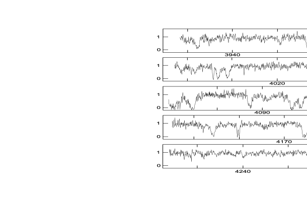
  Figure 2: Typical quasar spectrum with the Ly$\alpha$–forest of QSO 2206-199 N with high–resolution ($\Delta\lambda=0.09$Å), adapted from Pettini et al. [25].

  If the assumption of a universal shell structure in the distribution of galaxies is correct, we must expect large numbers of Ly$\alpha$ absorption lines. Each time the line of sight passes through a shell we can expect either a small absorption line or a whole group of blends, i.e. small lines, cramped together, separated by the internal peculiar velocities. The evidence from high-resolution spectra shows that the grouping of small lines into blends is caused by internal peculiar velocities typically of up to 300 km/s. See the spectra with high–resolution ($\Delta v$=6 km/s) from Pettini et al. adapted in Fig. 1 [25]. For the typical value of 300 km/s see also [7].

  The Hubble expansion of the shell structure must produce a characteristic pattern which is seen in the spectra up to redshifts of 4. There, the peculiar motions slowly begin to dominate the pattern as their effect on the line width grows with $(1+z)$. In order to determine a typical average diameter of the voids, we have to take averages over 200 Å , corresponding to 20 or 30 lines or close line groups. This then is interpreted as 20 or 30 shells. It yields the average void-diameter in $\Delta z$.

  

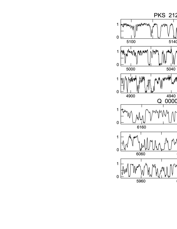
  Figure 4: Ly$\alpha$–forest spectra of two quasars a) PKS 2126-158 ($z_{\rm abs}=3.0...3.2$) and b) Q 0000-26 ($z_{\rm abs}=3.9...4.1$), adapted from Cristiani [7], as typcial examples at these redshifts.

  Fig. 2 shows some typical spectra from two quasars with redshifts 3.2 and 4.1, adapted from Cristiani [7]. Each interval of 200 Å yields one value of $\Delta z$ as function of the redshift factor $(1+z)$. From 21 quasar spectra with sufficiently high spectral resolution, we obtained 34 $\Delta z$-values from 1360 Ly$\alpha$ lines [15, 18, 19].

  Fig. 3 shows a schematic view of a lightray traversing 9 shells and the corresponding absorption spectrum.

  

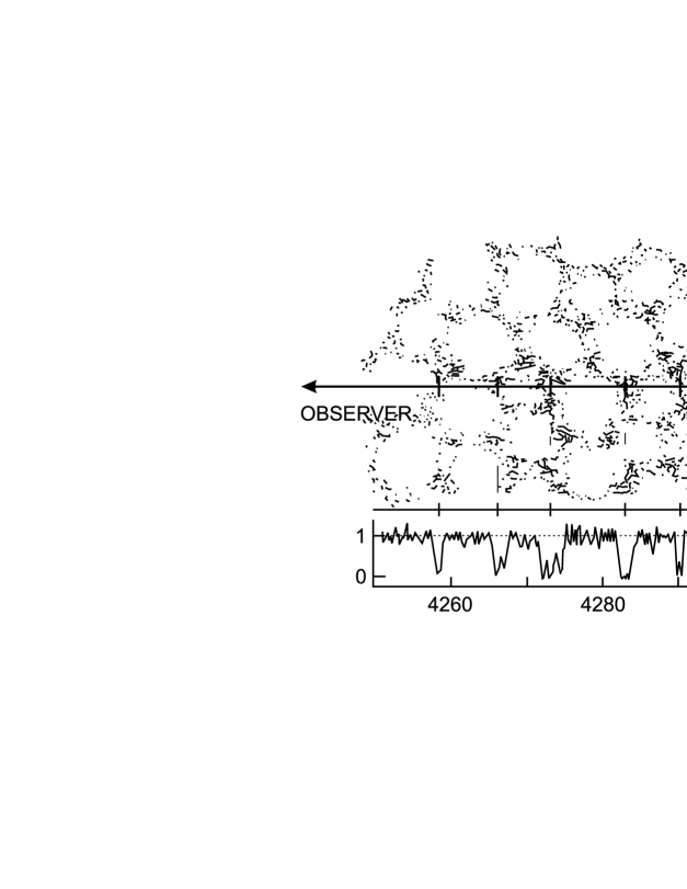
  Figure 6: A spongelike bubble structure in the spatial distribution of hydrogen in galaxies and intergalactic clouds and the corresponding Ly$\alpha$ absorption lines (schematic).

  Mathematics tells us that in a Friedmann universe the $\Delta z$-values are proportional to the Hubble expansion rate $H(t)$ at that time when the absorption takes place in the hydrogen cloud. Again, the time $t$ is being replaced by the redshift factor $(1+z)$. The lightray from the quasar traverses a void diameter $R(t)\cdot\Delta\chi$ along the radial coordinate $\chi$ in the time interval $\Delta t$:

  $$\Delta t=-\frac{1}{c}R(t)\cdot\Delta\chi.$$ (3)

  The corresponding redshift difference $\Delta z$ follows from $1+z=R_{0}/R(t)$:

  $$\Delta z=-\frac{R_{0}}{R(t)}H(t)\Delta t.$$ (4)

  Thus we have

  $$\Delta z=(R_{0}\cdot\Delta\chi)\frac{H(z)}{c}$$ (5)

  Thus, the squares of the observed $\Delta z$-values are directly proportional to the Friedmann equation. Here we use the convenient normalized form (see eq.(2)). From this we get a regression formula with three terms: $a_{0}$ corresponding to $\lambda_{0}$, $a_{2}$ corresponding to the curvature term and $a_{3}$ corresponding to the density parameter $\Omega_{M,0}$. Thus, $a_{3}$ must be positive. The regression formula for the observed $(\Delta z)^{2}$ is

  $$(\Delta z)^{2}=a_{0}+a_{2}(1+z)^{2}+a_{3}(1+z)^{3}.$$ (6)

  There is no $a_{1}$, no linear term in the Friedmann equation. This is a very lucky circumstance for the regression analysis. A regression without a linear term is highly unusual. Because of this property we named the method “Friedmann regression analysis”.

  The $(\Delta z)^{2}$-values are plotted versus the redshift factor in Fig. 4. The observed data cover a range from redshift 1.8 to 4.5. They must be represented by a curve which consists, at first, of a cubic parabola originating in the left corner at (0,0). Secondly, there must be a parabola with a negative $a_{2}$ opening into the downward direction. Both curves, together, form then the regression curve. It is remarkable and rewarding that the curve at zero-redshift yields $\Delta z\approx 0.009$, in agreement with the Harvard survey of the galaxy distribution in our neighbourhood (represented by the large rectangle in Fig. 4), showing the consistency with our basic assumption of the expanding shell structure.

  

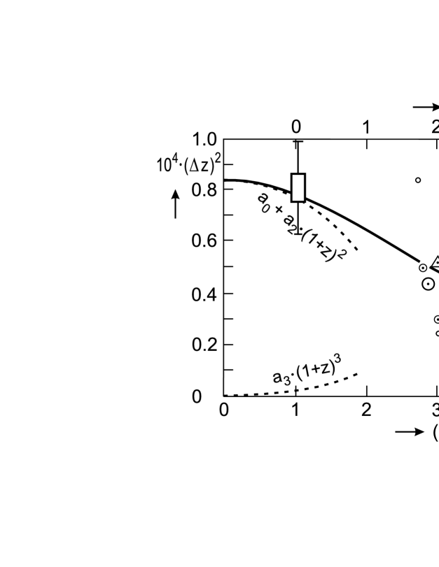
  Figure 8: Friedmann regression analysis of the observed ($\Delta z$)-values of the void–pattern in the redshift range 1.8 to 4.5 adapted from [15],[26].

  The results were quite a surprise to us. The Friedmann-Lemaître model is $\Lambda$-dominated and expands into infinity in a closed spherical metric ($\lambda_{0}=1.08$). The density parameter $\Omega_{M,0}=0.014$ corresponds to the total baryonic density derived from primordial nucleosynthesis by the Chicago group of the late Dave Schramm [31]. Thus, here is no place for a dominant contribution by non-baryonic matter. No place for exotic matter: a very provocative result!

  Fig. 5 shows the resulting Friedmann-Lemaître model, a closed model which expands into infinity. It was called the BN-P (Bonn-Potsdam)-model by “Sterne und Weltraum”, the German “Sky and Telescope” [5]. Fig. 5 also shows the pure baryonic Standard Sandage-Tammann–model, with $\Lambda=0$ and an open hyperbolic metric and $\Omega_{M,0}=0.03$ (pure baryonic) [30]. In addition, there is the Einstein-de Sitter model, the curve on the left, and the flat Ostriker-Steinhardt–model with $\Omega_{M}(t)+\lambda(t)=1$ nearly throughout the past [22]. The stars designate the points of inflection in the $\Lambda$-models. The circle on our BN-P curve shows the time, when the density parameter was larger than 4 in the loitering phase (see Fig. 8). At that time the curvature radius was $R=1/\sqrt{\Lambda}=6$ Gly at a Friedmann time of 7 Gigayears. The loitering phase provides an excellent basis for galaxy formation, because structures grow almost exponentially in this epoch.

  

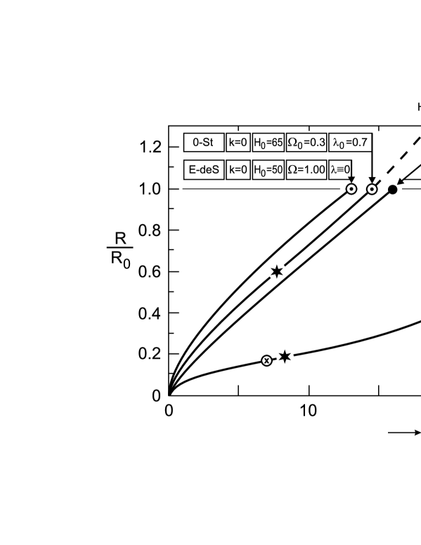
  Figure 10: Evolution of the normalized scale factor for four cosmological models with the cosmological parameters marked on each curve (see text).

  Our paradigm of a shell structure expanding primarily with the Hubble flow has resulted in a value of the density parameter, which could be considered as the possible minimum value. Thus, the corresponding age of about 30 Gigayears would count as an upper limit for the age of the universe. In that case all the early generations of stars would have burned out by now, leading to a cosmos with huge numbers of black dwarfs or neutron stars.

  One might argue that we neglected evolution in the shell structure. This could cause a somewhat too small matter density. But it is hard to see that $\Omega_{M,0}$ could be larger than 0.05, still in the Chicago regime. With a density parameter of 0.05 we could bring the cosmic age down somewhat, but hardly below 25 Gigayears. If $\Omega_{M,0}$ would be as large as 0.3, or even larger, then the Ly$\alpha$–forest must be interpreted in another way, see e.g. [20, 21].

  Supporting evidence for a more or less regular shell structure in the spongelike distribution comes from the fact, that about 30 percent of the quasars show somewhere in their spectra a very wide absorption line of about 40 Å with a Doppler width of up to 3000 km/s. These lines are optically thick, but with interesting structures in the wings. Usually the lines are called “damped Ly$\alpha$–lines”, believed to be due to huge, hot clouds of almost the size of a galaxy. Here we shall present an alternative explanation, which comes about very naturally with our paradigm of a universal shell structure.

  On the line of sight from the quasar toward the observer it will occasionally happen, that the line cuts tangentially through a shell, going through many clouds, which produce a large number of Ly$\alpha$-lines cramped together, but spread by the motions of the individual clouds over a range of 3000 km/s, the typical expansion-speed of the voids.

  This explanation is supported by a pair of two quasars [6]. They are separated on the sky by 8 arcmin. They are not physically related. Their redshifts are different (3.17 and 3.23). Their spectra were taken by Paul Francis and Paul Hewitt [12]. These spectra show twice a very wide absorption line at the same wavelength: one pair at 4110 Å and the other pair at 4690 Å . This occurred despite the fact that their lines of sight are separated by more than 10 Mpc at the positions of the absorbing clouds.

  

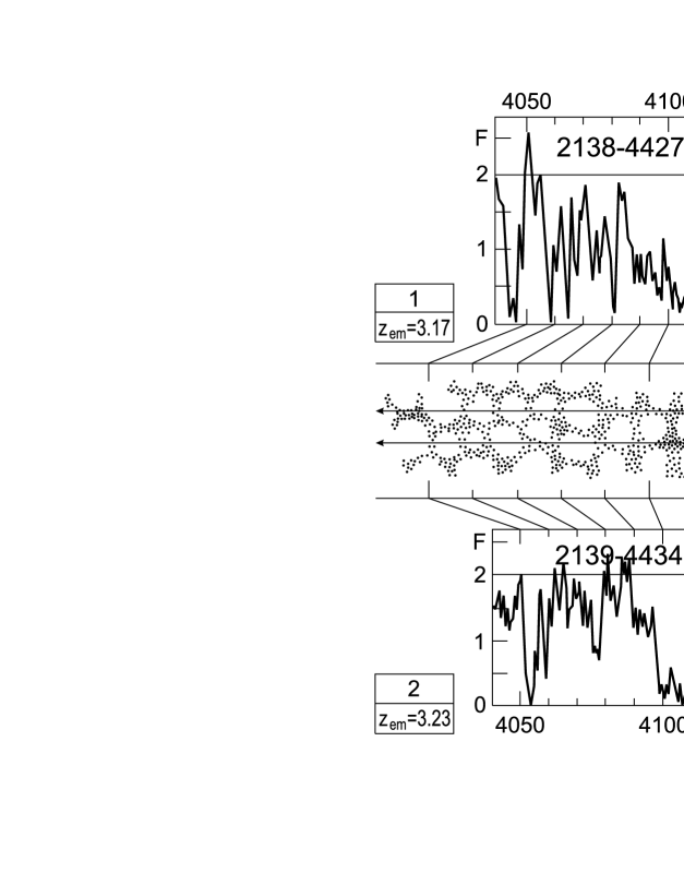
  Figure 12: A pair of very wide absorption lines occurs in the Ly$\alpha$–forest of two quasars at coinciding wavelengths, centered at 4110 Å. A similar pair (B) occurs at 4685 Å. The center part shows schematically our interpretation of the shell structure of hydrogen clouds along the two lines of sight, separated by 8 arcmin on the sky.

  In Fig. 6 we show the part (pair (A)) with the very wide lines around 4100 Å in both spectra, quasar 1 on top, quasar 2 below. In the middle, a schematic shell structure is drawn on scale, corresponding to the redshift distance of $z$ = 2.380. A very similar pair (B) of wide lines is found at $z$ = 2.853. It seems to us, that these two coincidences of two pairs of very wide spectral lines support strongly our explanation. We do not have to evoke special superlarge clouds. The tangential cuts through a shell on both sides easily explain the observations.

  The low, pure baryonic density with $\Omega_{M,0}=0.014$ contradicts the results from the gravitational instability theory, which yields higher densities, pointing to a dominant contribution by non–baryonic, exotic dark matter. As an example we show in Fig. 7 Friedmann-Lemaître models with $\Omega_{M,0}=0.2$. It implies that perhaps 90 percent of the mass is in the form of non–baryonic, exotic particles. This confronts us with the fundamental problem: What is the universe made of? Do we need a dominance by exotic matter or can the universe be baryonic, if it is sufficiently old and most of the stars are already dead bodies or neutron stars? This density parameter (0.2) was recently derived by Neta Bahcall from the distribution of clusters of galaxies [1]. The curve with $\lambda_{0}=0.8$ in Fig.7 shows her preference for a flat $\Lambda$-model with an age of 14 Gyrs (with $H_{0}$ = 75 km/(s Mpc)).

  We should, however, not neglect the closed models. The situation at the Planck-time in the very early universe can be reasonably understood only in a closed model with spherical metric. Thus, we should consider closed models in particular: Here we discuss the curve with $\lambda_{0}=1.4$ and an age of 22 Gigayears for $H_{0}$ = 75 km/(s$\cdot$Mpc). In this model (marked 2 in Fig.8) at a Friedman time of 7 Gigayears the density parameter went through its maximum with $\Omega_{M}$ = 4 and a corresponding value of $R_{\Lambda}=1/\sqrt{\Lambda}$ of 6.4 Gly, about the same value as in our BN-P-model.

  

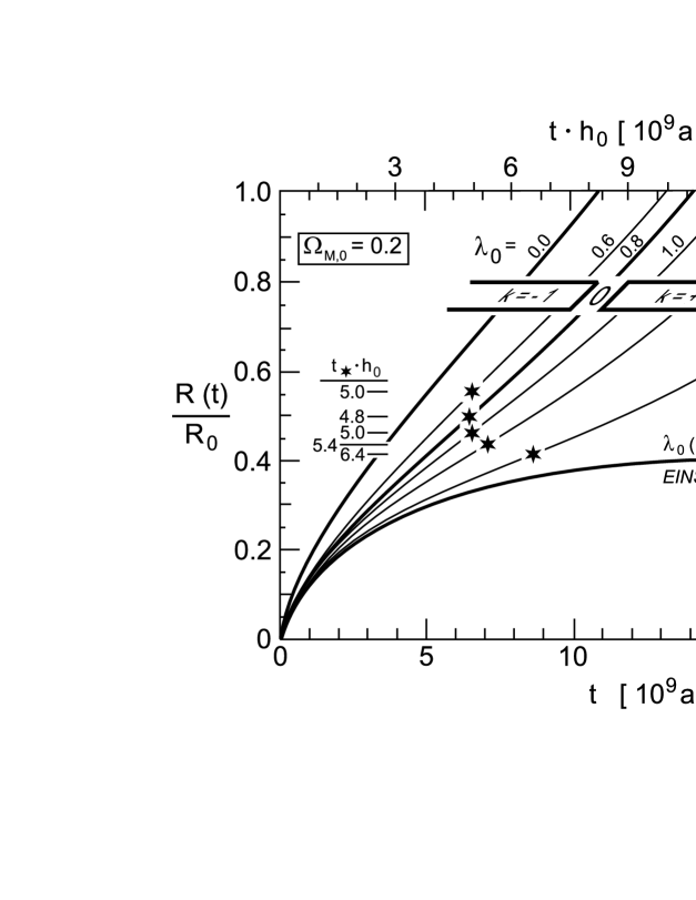
  Figure 14: Examples of models $R(t)/R_{0}$ as function of time for $\Omega_{M,0}=0.2$ with a dominant amount of non–baryonic matter.

  In Fig. 8 the evolution of $\Omega_{M}(t)$ and $\lambda(t)$ is shown for the closed model (marked 2) and the flat model (marked 3). The evolution is shown together with our pure-baryonic BN-P model (marked 1). In flat models the density parameter sticks to the straight line representing a fine tuning. Its value remains below 1 throughout. The two curves of the closed, $\Lambda$-dominated models (marked 1 and 2) provide sufficient time for galaxy formation at redshifts between 2 and 6 during the loitering phase, even in a pure baryonic, low density model without cold dark matter. Of course, this model would be a “top down model” of structure formation, because the Jeans–mass is as large as the mass of a massive galaxy cluster and the galaxies have to fragment out of this material (if adiabatic perturbations where present in the early universe).

  

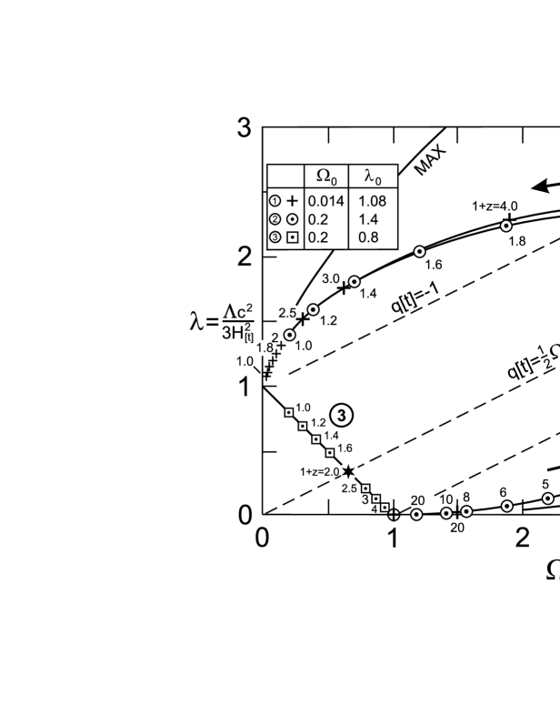
  Figure 16: Evolution of the cosmological parameters in the $\Omega(t)$, $\lambda(t)$ plane for a flat model (3) and two models (1), (2) with spherical metric. The time $t$ is represented by $(1+z)$. For further details see the text.

  

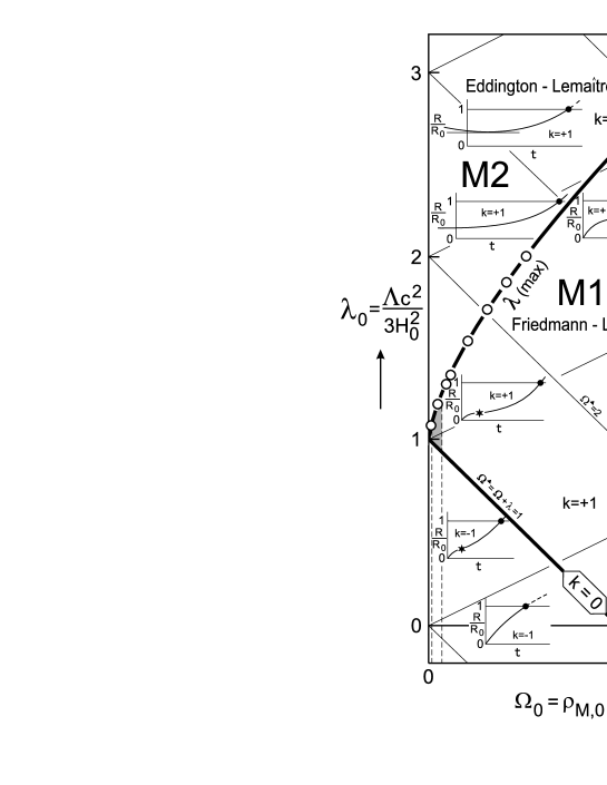
  Figure 18: Classification of Friedmann models as function of the present matter density parameter $\Omega_{0}$ and the cosmological term $\lambda_{0}$. The “Einstein–limits” ($\lambda_{0}(max)$ and $\lambda_{0}(min)$) give the limits for Friedmann’s M1 models. The two dashed lines on the left side show the range of the baryonic density ($0.01...0.06$), derived from the primordial nucleosynthesis. The figure is adapted from Blome, Priester (1991) [3].

  This leaves us with the question whether the paradigm of the simple gravitational instability theory (due to adiabatic perturbations) is really sufficient and whether it is a complete theory for the explanation of structure formation, in particular of the spongelike shell structure. How much of exotic, non-baryonic matter is really necessary? What is it percentage-wise? At the present time this remains an unsolved problem. On the other hand, if the simple theory of structure formation due to adiabatic perturbations (leading to $\Omega_{M,0}\geq 0.2$) turns out to be right, the Ly$\alpha$-forest has to be interpreted in another way.

  Recently, Fukugita, Hogan and Peebles reconsidered the cosmic baryon budget in an extensive study [14]. Their fair accounting yields as a reasonable value for the net baryon density parameter $\Omega_{B,0}=0.021\pm 0.007$ for $h=0.7$ or $(0.015\pm 0.005)h^{-1}$. This agrees reasonably well with $\Omega_{B,0}=(0.0125\pm 0.0025)h^{-2}$ from the primordial nucleosynthesis [31]. The density parameter of the gravitational mass including non–baryonic dark matter remains debatable. With the assumption that the mass to spheroid light ratio (with luminosity in the B–band) $M/L_{B}=(270\pm 60)h$ is universal i.e. applicable to the majority of field galaxies, Fukugita et al. derive $\Omega_{M,0}=0.18+0.07,-0.05$. The field galaxies outnumber the compact cluster galaxies by a factor between 10 and 20. From the flat rotation curves of field galaxies a typical value $M/L\approx 20h$ in solar units was generally obtained. Applying this value to the field galaxies yields $\Omega_{M,0}=0.013\pm 0.004$, in good agreement with $\Omega_{M,0}=0.014$ from our Ly$\alpha$ analysis. This result supports a conclusion that the mass of the universe is dominated by the baryons. It would further imply that the evolution in the compact clusters proceeded much earlier or faster as compared to the field galaxies. A loitering phase in the Friedmann models would probably favour the different evolution efficiencies (see the investigation by Feldman and Evrard of structure formation in a loitering universe [11]).

  Recent estimates of cosmological parameters show a preference for low–density, $\Lambda-$dominated models, see for instance the analysis of high–redshift supernovae [28] or the analysis of classical double radio galaxies [17]. Euclidian space metric is often assumed in these cases with $\Omega_{M}(t)+\lambda(t)\equiv 1$, as the analysis does not provide a specific value for $\lambda_{0}$. In our analysis of the Ly$\alpha$–forest, using as a basic assumption a shell structure expanding predominately with the Hubble flow, both parameters ($\Omega_{M,0}=0.014\pm 0.006$ and $\lambda_{0}=1.08\pm 0.02$) were derived with small errors (Friedmann regression analysis) [15]. This provides significant evidence for a low–density, closed, $\Lambda$–dominated model with spherical metric, expanding forever. These models belong to the Friedmann–Lemaître models (M1) (see Fig. 9). In 1922 Friedmann named them: “Monotone Weltmodelle der ersten Art” [13].

  Albert Einstein wrote in 1954: “Besonders befriedigend erscheint die Möglichkeit, daß die expandierende Welt räumlich geschlossen sei, weil dann die so unbequemen Grenzbedingungen für das Unendliche durch die viel natürlichere Geschlossenheitsbedingung zu ersetzen wäre” [10]. In short: The conditions for a closed cosmos are much more natural than the inconvenient, uncomfortable boundary conditions for the infiniteness in an unlimited universe.

  Acknowledgements: We are grateful to Bulent Uyanıker for his careful reading of the manuscript and for useful discussions. Our special thanks go to Prof. Hans Volker Klapdor–Kleingrothaus for the invitation to “dark98”, Heidelberg, July 20–25, 1998. C.v.d.B. was supported by the Deutsche Forschungsgemeinschaft (DFG) and the Max–Planck Gesellschaft.

References

- [1] Bahcall, N., preprint astro-ph/9711062 (1997)
- [2] Blome, H.J., Hoell, J., Priester, W., Kosmologie, Chap. 4 in Bergmann–Schaefer: Lehrbuch der Experimentalphysik, Band 8: Sterne und Weltraum, p.311–427 W. de Gruyter, Berlin (1997)
- [3] Blome, H.J., Priester, W., A&A 250, 43 (1991)
- [4] Bothun, G., Modern Cosmological Observations and Problems, Taylor and Francis, London (1998)
- [5] Bruck, C. van de, Sterne und Weltraum 34, 529 (1995)
- [6] Bruck, C. van de, Priester, W., in Clusters, Lensing, and the Future of the Universe, ASP. Conf. Ser. 88, 290 (1996)
- [7] Cristiani, S., Preprint ESO SP 1117 (1996); Cristiani, S., D’Odorico, S., D’Odorico, V., Fontana, A., Giallongo, E., Savaglio, S., MNRAS 285, 209 (1997)
- [8] Carroll, S.M., Press, W.H., Turner, E.L., Ann. Rev. Astron. Astrophys. 30, 499 (1992)
- [9] see http://www.mpa-garching.mpg.de/ jgc/
- [10] Einstein, A., Grundzüge der Relativitätstheorie, Vieweg-Verlag (1956)
- [11] Feldman, H.A., Evrard, A.E., Int. Journ. Mod. Phys. D 2, 113 (1993)
- [12] Francis, P., Hewitt, P., Astron. Journ. 123, 1066 (1993)
- [13] Friedmann, A., Z. Phys. 10, 377 (1922)
- [14] Fukugita, M., Hogan, J.C., Peebles, P.J.E., ApJ 503, 518 (1998)
- [15] Hoell, J., Liebscher, D.E., Priester, W., Astron. Nachr. 315, 89 (1994)
- [16] Geller, M., Huchra, J., Science 246, 897 (1989)
- [17] Guerra, E.J., Daly, R.A., Wan, L., astro–ph/9807249 (1998)
- [18] Liebscher, D.E., Hoell, J., Priester, W., A& A 261, 377 (1992a)
- [19] Liebscher, D.E., Priester, W., Hoell, J., Astron. Nachr. 313, 265 (1992b)
- [20] Muecket, J.P., Petitjean, P., Kates, R.E., Riediger, R., A&A 308, 17 (1996)
- [21] Machacek, M.E., Bryan, G.L., Anninos, P., Norman, M.L., astro–ph 9808029 (1998)
- [22] Ostriker, J.P., Steinhardt, P.J., Nature 377, 600 (1995)
- [23] Padmanabhan, T., Structure formation in the universe, Cambridge University Press (1993)
- [24] Persic, M., Salucci, P., MNRAS 258, 14P (1992)
- [25] Pettini, M., Hunstead, R.W., Smith, L.J., Mar, D.P., MNRAS 246, 545 (1990)
- [26] Priester, W., Hoell, J., Liebscher, D.E., Bruck, C. van de, Proc. Third Alexander Friedmann Internat. Sem. on Gravitation and Cosmology (ed. Gnedin, Grib, Mostepanenko), p.52–67, Friedmann Lab. Publ. St. Petersburg (1996)
- [27] Priester, W., Hoell, J., Bruck, C. van de, in Clusters, Lensing, and the Future of the Universe, ASP. Conf. Ser. 88, 286 (1996)
- [28] Riess, A., et al., astro-ph/9805201, to appear in the Astronomical Journal (1998)
- [29] Salucci, P., Persic, M., preprint astro–ph/9601018 (1996)
- [30] Tammann, G., Rev. Mod. Astronomy 9, 139 (1997)
- [31] Walker, T.P., Steigmann, G., Schramm, D., Olive, K., Kang, H.S., ApJ 376, 51 (1991)
- [32] Weinberg, S., Rev. Mod. Phys. 61, 1 (1989)
- [33] Weinberg, S., The dreams of a final theory, Pantheon Books, New York (1993)