HST OBSERVATIONS OF THE BROAD ABSORPTION LINE QUASAR PG 0946+301

Abstract

We analyze HST and ground based spectra of the brightest BALQSO in the UV: PG 0946+301. A detailed study of the absorption troughs as a function of velocity is presented, facilitated by the use of a new algorithm to solve for the optical depth as a function of velocity for multiplet lines. We find convincing evidence for saturation in parts of the troughs. This supports our previous assertion that saturation is common in BALs and therefore cast doubts on claims for very high metallicity in BAL flows. Due to the importance of BAL saturation we also discuss its evidence in other objects. In PG 0946+301 large differences in ionization as a function of velocity are detected and our findings supports the hypothesis that the line of sight intersects a number of flow components that combine to give the appearance of the whole trough. Based on the optical depth profiles, we develop a geometrical-kinematical model for the flow. We have positively identified 16 ions of 8 elements (H I, C III, C IV, N III, N IV, N V, O III, O IV, O V, O VI, Ne V, Ne VIII, P V, Si IV, S V, S VI) and have a probable identifications of Mg X and S IV. Unlike earlier analysis of IUE data, we find no evidence for BALs arising from excited ionic states in the HST spectrum of PG 0946+301.

Key words: quasars: absorption lines

1 INTRODUCTION

Broad absorption troughs associated with prominent resonance lines such as C IV $\lambda$1549, Si IV $\lambda$1397, N V $\lambda$1240, and Ly$\alpha$ $\lambda$1215 appear in about 10% of all radio quiet quasars (Foltz et al. 1990). These troughs are known as broad absorption lines (BALs) and are commonly attributed to material flowing out from the vicinity of the central engine. Typical velocity widths of the BALs are $\sim 10,000$ km s^-1 (Weymann, Turnshek, & Christiansen 1985; Turnshek 1988) with terminal velocities of up to 60,000 km s^-1. These high terminal velocities are seen in H1414+089 (66,000 km s^-1, Foltz et al. 1983) and in Q1231+1320 (58,000 km s^-1, spectrum from Korista et al. 1993). The percentage of BALQSOs among all quasars combined with the assertion that the flow covers $\mathrel{\raise 1.29167pt\hbox{$<$}\mkern-14.0mu\lower 2.58334pt\hbox{$\sim$}}0.2$ of the sky on average as viewed from the nucleus of the QSO (Hamann, Korista, & Morris 1993), suggests that all QSOs have BAL flows. This conclusion is supported by the similarity of the broad emission lines (BELs) in the spectra of BALQSOs and non-BALQSOs (Weymann et al. 1991). The BAL region is probably situated further away from the continuum source than the broad emission line region based on the attenuation of the BELs by the BALs (Junkkarinen, Burbidge, & Smith 1983; Turnshek 1988; for alternative view see Murray et al. 1995). Radiative acceleration probably governs the dynamics of the flow (Arav, Li & Begelman 1994; Murray et al. 1995; de Kool & Begelmen 1995; Arav et al. 1995)

Establishing the physical properties of the flow by determining the ionization equilibrium and abundances (IEA) of the BAL material is a fundamental issue in BALQSOs studies. Data from HST are crucial in trying to answer these questions. Ground based observations show only a small number of BALs (most of which are listed above) that arise from different elements. HST observations of moderate to high redshift ($z=1-3$) objects allow us to access the 500–1000 Å rest-wavelength region which contains many more BALs, including BALs from different ions of the same element, and even different BALs from the same ions. Without data on BALs from different ions of the same element the effects of ionization and abundances are very difficult to decouple. The first and heretofore the most comprehensive study of a BALQSO using HST data was done by Korista et al. (1992, hereafter K92) on BALQSO 0226–1024. In the combined HST and ground based spectrum at least 12 different absorbing ions were identified including the following CNO ions: C III, C IV, N III, N IV, N V, O III, O IV, O VI. Several groups (Korista et al. 1996; Turnshek et al. 1996; Hamann 1996) have used these data in their IEA studies while introducing innovative theoretical approaches to the problem.

However, these works suffer from large uncertainties, which comes from reliance on apparent integrated ionic column densities ($N_{ion}$). Accurate $N_{ion}$ are crucial because inferences on the IEA in the BAL region are derived by trying to simulate BAL column densities using photoionization codes. The problem is that the measured apparent optical depths in the BALs (defined as $\tau=-ln(I_{r})$, where $I_{r}$ is the residual intensity seen in the trough) cannot be directly translated to realistic $N_{ion}$ due to loose constraints on the covering factor and level of saturation (see discussion in K92). We note that the term “covering factor” is defined in this paper as the portion of the radiating source covered by the flow as seen by the observer. This is to be distinguished from the percentage of solid angle which the flow covers as viewed fron the nucleus of the QSO. Arav (1997) has demonstrated that in the case of BALQSO 0226–1024 the major BALs are very probably saturated although not black. If the BALs are saturated, the inferred $N_{ion}$ are only lower limits, and thus the previous conclusions regarding the IEA in this object, and by extension in all BALQSOs, are very uncertain. By now the body of evidence for non-black BAL saturation has grown considerably and in § 4.2 we discuss these in detail.

Therefore, a crucial step in BAL IEA studies is a careful analysis of the BAL profiles aimed at determining the real optical depths and thus real column densities. In order to do so we have to abandon the use of integrated column densities. Different parts in the BALs can (and do, see below) show different levels of saturation and covering factors, and the apparent optical depths show velocity-dependent ionization changes. Supporting evidence comes from the so called mini-BALs, which are defined as intrinsic absorbers with velocity width smaller than 2000 km s^-1, whereas traditional BALs are wider then 2000 km s^-1(Weymann et al. 1991). Mini-BALs show large variation in covering factor on scales of hundreds of km s^-1 (Barlow 1997). Thus, in order to shed light on the IEA of BAL flows, there is no substitute for a detailed study of optical depth as a function of velocity ($\tau(v)$) for as many BALs as possible in a given object.

Figure 1: Composite spectrum of PG 0946+301, flux is measured in the observed frame.

To this effect, we analyze the spectrum of PG 0946+301, which was discovered by Wilkes (1985) and observed in the UV by Pettini and Boksenberg (1986) using the IUE satellite. This object is by far the most suitable for such an analysis. From all the BALQSOs that were observed with HST it is the brightest with observable lines down to 570 Å rest frame, and has at least five times higher UV flux, shortward of 1000 Å rest frame, than any observed object. Unlike the cases of BALQSO 0226–1024 and a few other BALQSOs in the HST archive, the flux of PG 0946+301 does not diminish rapidly shortward of 1000 Å. Another important advantage is that due to its low redshift (z=1.223), the Ly$\alpha$ forest in the spectrum of PG 0946+301 is much less dense than in other observed BALQSOs and therefore the BALs are less contaminated with unrelated absorption. These advantages are crucial since in order to make a detailed $\tau(v)$ analysis much higher quality “clean” data are needed than for the apparent-$N_{ion}$ approach. This analysis is based on a new algorithm we developed that enables us to solve for the optical depth of the line whether it is a doublet, triplet or higher order multiplet. Solving for multiplets other than doublets was not possible with the algorithm published by Junkkarinen et al. (1983; which was also used in a modified way by K92). Our algorithm is also more stable and can be used to extract apparent-optical depth under saturated conditions. Grillmair & Turnshek (1987) used a different algorithm, but give too few details to allow a comparison. We give a detailed description of our optical depth solution method in Appendix A.

Supplementing the $\tau(v)$ analysis we also present results from the traditional apparent-$N_{ion}$ approach. This is done for two reasons. First, there are regions in the spectrum where several BALs are blended together and therefore a $\tau(v)$ analysis in these region is impossible. In these regions the $N_{ion}$ analysis allow us to obtain reasonable estimates for the existence and importance of different BALs. Second, the quality of available data is much lower shortward of 750 Å (rest frame). and does not allow a detailed $\tau(v)$ analysis. Several important lines reside in that part of the data and our only inferences about them can be obtained by the apparent-$N_{ion}$ analysis.

The plan of the paper is as follows: In § 2 we describe the data acquisition and reduction. In § 3 we analyze the apparent optical depth of the BALs. Evidence for non-black saturation in PG 0946+301 is presented in § 4 supplemented by a summery of evidence from other objects. Results from the integrated $N_{ion}$ approach (template fitting procedure) are given in § 5. A kinematic model for the flow is presented in § 6. In § 7 we discuss the significance of these findings and address the meta-stable lines issue. Appendix A describes the methods to extract $\tau(v)$ for different lines, and Appendix B identifies the non-BAL absorption seen in the spectrum.

2 DATA ACQUISITION AND REDUCTION

HST FOS observations of PG 0946+301 were made on 16 February 1992 as part of the FOS GTO program. A low resolution spectrum was obtained with the FOS Blue side using the rapid mode, the G160L grating, and the 1.0" aperture. The integration time with the G160L was 1768 seconds. The G160L spectrum has a FWHM resolution of about 8.0 Å and a sampling of about 1.74 Å per pixel. Observations were obtained with the FOS Red side on the same date with both the G190H and G270H gratings with the 1.0" aperture and exposure times of 4441 and 2663 seconds respectively. The G190H resolution is 1.5 Å FWHM with 0.36 Å per pixel sampling and the G270H resolution is 2.2 Å FWHM with 0.51 Å per pixel sampling. The usual reduction procedure was used to generate flux as a function of wavelength. The G160L Blue and G190H Red observations were corrected for particle background and any wavelength independent scattering using spectral regions where the sensitivity is essentially zero. The data were corrected for detector and spectrograph sensitivity variations using flat field observations close in time to the actual observations. Since the flat fields of the FOS vary in time, the flat field corrections sometimes leave residual features. In these observations, there are no apparent spurious features due to flat field variations. Spectra from the three HST gratings were combined to obtain a full HST spectrum. The relative wavelength determination was done by using common features at the edges of the gratings. We estimate the relative wavelength error to be less than half a pixel width. The absolute wavelength calibration was determined by the Galactic Mg II absorption lines seen in the G270H grating, assuming they lie at their vacuum wavlengths in the frame of our Galaxy.

Optical observations of PG 0946+301 were made at Lick Observatory on 28 March 1992 (UT) using the Kast double spectrograph system on the Shane 3m telescope. A 3000s observation was obtained using the blue side of the spectrograph with a 600 line mm^-1 grism blazed at 4310 Å. The spectrum has a useful wavelength range of 3150 – 5250  Å with a resolution of about 5 Å FWHM. The usual optical reduction procedures were followed using the VISTA reduction package.

3 ANALYSIS OF THE BALs APPARENT $\tau(v)$

In Figures 2 we present $\tau(v)$ solutions for seven BALs. A detailed description of the method used to extract these solutions from the data is given in appendix A. In this section we describe and analyze the apparent optical depth solutions. The apparent $\tau(v)$ is extracted under the assumptions that the source is completely covered, and that the bottoms of the troughs are not filled-in by scattering or some other light source. We identify two major components (A and B) and three minor components (C, D and E) in the flow. In figure 2 the $\tau(v)$ are organized according to the ionization energy needed to destroy the ion, with the highest ionization stage at the top.

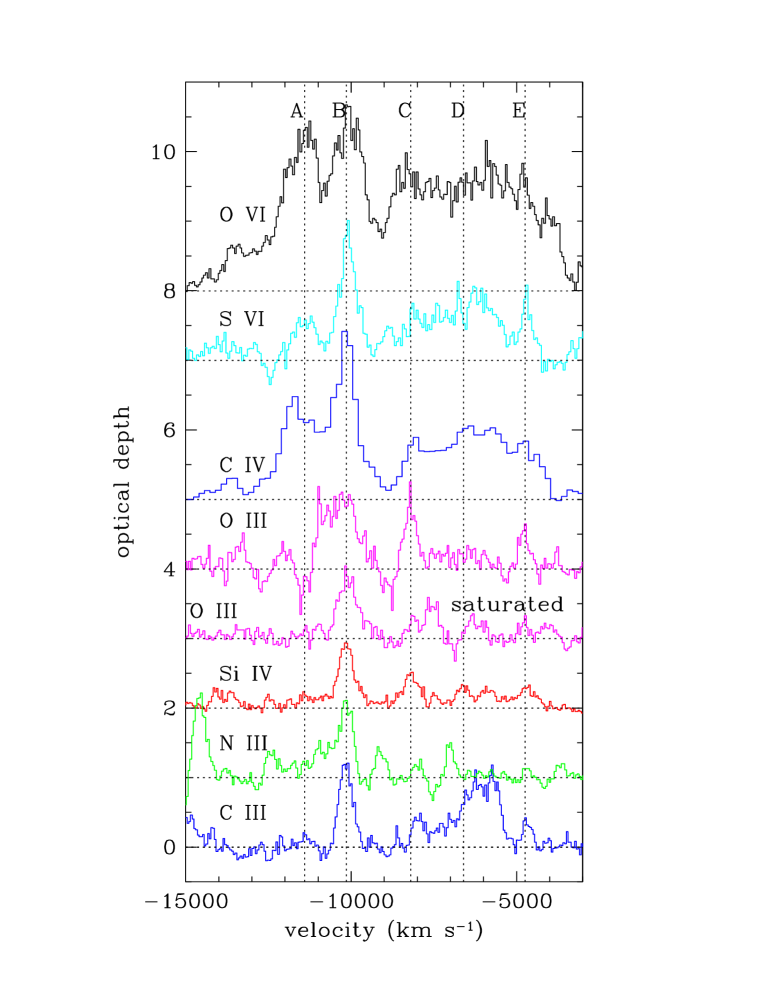
Figure 2: $\tau(v)$ for seven lines. The horizontal dotted line at the base of each $\tau(v)$ mark the $\tau=0$ for this line. Vertical dotted lines identify the components discussed in the text. Both an optically thin and a saturated solution of O III are shown (see § 4.1). For presentation purposes each solution is shown with a $\Delta\tau=1$ offset with respect to the one beneath it. The exception is S VI which for clarity has an offset of $\Delta\tau=2$ from the C IV solution.

3.1 The Different Components

Component A is clearly detected only in the high ionization lines: O VI, S VI and C IV. It is strongest in O VI ($\tau_{max}=2.3$), where its width is 1200 km s^-1. In S VI component A is very similar in shape and position to the O VI one with $\tau_{max}=0.6$. Across most of component A profile $\tau_{\scriptscriptstyle O~{}VI}/\tau_{\scriptscriptstyle S~{}VI}\simeq constant$, this is in contrast to the situation in Component B (see Fig. 3 and discussion below). A small difference is seen at high velocity where the O VI seems to be somewhat more extended. In C IV component A is also strong ($\tau_{max}=1.3$), but the location of the peak is shifted by $\sim$400 km s^-1 to the blue with respect to those of O VI and S VI. However, the C IV data has lower resolution than the HST data and the position of the peak is based on only two pixels. C III and Si IV show marginal optical depth at the velocity position of component A and the other low ionization lines have $\tau(\mbox{A})\simeq 0$.

Component B is the most prominent feature in each BAL. The width of component B differs substantially in different lines. In the high ionization lines O VI and C IV the full-width-half-maximun (FWHM) of component B is 1100 and 800 km s^-1 respectively, whereas in the low ionization lines the FWHM is $\simeq$500 km s^-1 with very similar component profile. However, the S VI line does not adhere to the separation based on ionization scheme. Although S VI ionization potential is higher than that of C IV, its component B profile is very similar to the profiles seen in the low ionization lines (see Fig. 3).

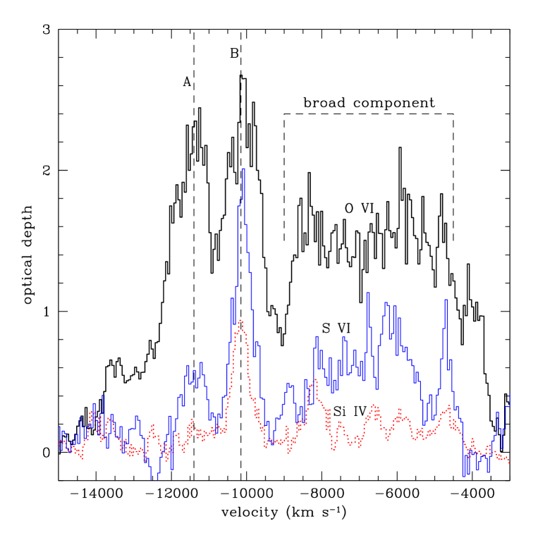
Figure 3: $\tau(v)$ for O VI, S VI and Si IV, where the main components of the flow are marked.

Being a singlet, the C III line provides the most reliable profile for component B. It is reassuring that the profiles of component B in Si IV, saturated O III (see § 4.1) and S VI are essentially identical with that of C III (within the quality of the data and the uncertainties about the continuum level). The excess optical depth in C III near 6000 km s^-1 is due to the N III BAL. Component B in N III shows a deviation from this profile on its blue wing, which is probably due to blending with component D of C III.

Component C does not stand out above the smooth, broad absorption in O VI, S VI and C IV. It is strong in Si IV, and may possibly be associated with weak features in N III, C III and saturated O III with a small shift ($\sim 200$ km s^-1) to the red. The strong feature in the unsaturated O III profile is most likely due to the deconvolution procedure, and shows clearly the major effects that deconvolution with inapropriate line ratios can introduce. Component D is only seen in C IV and Si IV, and may be spurious. Component E is clearly seen in all seven BALs. The relatively strong E component in S VI might be partially due to component B of P IV $\lambda$951, but the evidence is not strong enough for a clear identification of this BAL. Components C, D and E are significantly narrower than components A and B.

3.2 Ionization as function of velocity

We find strong ionization changes as a function of velocity in the apparent optical depth of different lines. The most striking difference is seen in component A, which is strong in the high ionization lines: O VI, C IV, S VI, but is very weak or absent from the low ionization lines Si IV, N III and C III. A lower limit for the optical depth ratio in component A is $\tau_{\scriptscriptstyle O~{}VI}/\tau_{\scriptscriptstyle Si~{}IV}\mathrel{\raise 1.29167pt\hbox{$>$}\mkern-14.0mu\lower 2.58334pt\hbox{$\sim$}}10$. This is in contrast with component B which appears in all lines and is only twice as strong in the high ionization lines as in the low ionization lines. We conclude that in PG 0946+301 the apparent ionization has a strong dependence on velocity. However, the actual physical situation is more complicated since component B is saturated in all lines (see § 4.1). It is therefore possible that the ratios of real optical depths show less dependence on velocity.

A better diagnostic for the behavior of the real optical depth ratio is available from the broad component between –9000 km s^-1 and –4500 km s^-1 (see Fig. 3), which encompasses components C, D and E. This component is much more prominent in the high ionization lines. It is deepest in O VI with roughly a constant $\tau=1.5$. The high, flat-topped profile suggests that the line is saturated, and that the remaining flux at the bottom of the absorption trough comes either from a part of the continuum source that is not completely covered (partial covering) or consists of scattered light. For brevity, we refer to this combination of effects as “saturation”. In C IV and S VI the optical depth of the broad component is not constant, but is still substantial ($\overline{\tau}\simeq 0.8$ and 0.6 respectively). Neither the $\tau(v)_{\scriptscriptstyle S~{}VI}/\tau(v)_{\scriptscriptstyle Si~{}IV}$ nor the $\tau(v)_{\scriptscriptstyle C~{}IV}/\tau(v)_{\scriptscriptstyle Si~{}IV}$ ratios for this feature are approximately constant. This behavior is indicative of large variation in real $\tau(v)$ ratios since the S VI and C IV are probably not strongly saturated. Ionization changes as a function of velocity are the simplest explanation for non-proportional $\tau(v)$ once saturation is not the main culprit.

4 EVIDENCE FOR NON BLACK SATURATION

4.1 Evidence for saturation and partial covering in PG 0946+301

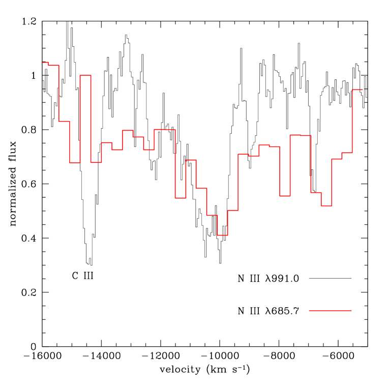
Figure 4: Residual intensity of the two N III BALs presented on the same velocity scale. The multiplet at 685 Å should have an optical depth 2.3 times larger than the 991 Å multiplet. Although the data for the 685 Å BAL are of inferior quality, it is clear that the apparent optical depth of both multiplets are equal within the errors. This 1:1 ratio for the residual intensity in the two multiplets is a direct evidence for non-black saturation in the BALs of PG 0946+301.

4.1.1 Optical depth ratio of the N III BALs

The best diagnostic for non-black saturation comes from comparing the optical depth of two BALs from the same ion. Transitions from the same ion should have a $\tau$ ratio equal the ratio of their $g_{i}f_{ik}\lambda$ (where $g_{i}$ is the degeneracy of the level, $f_{ik}$ is the oscilator strength of the transition and $\lambda$ is the transition’s wavelength). This $\tau$ ratio should not depend on the ionizing flux, density, colisional processes, ionization equilibrium or adundeces of the flow. In the PG 0946+301 data we have two unambiguos occurences of two BALs from the same ion. Two O III BALs (834 Å and 703 Å) are detected but the ratio of their $g_{i}f_{ik}\lambda$ is 1:1.1 and therefore they cannot be used as saturation diagnostic since they are expected to have very similar $\tau$. A good saturation diagonstic is found in the observed N III BALs (685 Å and 991 Å) which have $(g_{i}f_{ik}\lambda)_{685}/(g_{i}f_{ik}\lambda)_{991}=2.3$. In figure 4 we show the two N III BALs on the same velocity scale. It is evident that the residual intensities of component B in both BALs ($\sim 10,000$ km s^-1) are the same within the quality of the data. However, based on the residual intensity of N III 991 Å (0.4) the residual intensity of N III 685 Å should have been 0.12.

Before we can establish the ratio of apparent $\tau$ in the N III BALs as evidence for non-black saturation, we should examine possible caveats. If the absorption feature is significantly narrower than the spectral resulotion, then the observed trough would be shallower than expected. Data of the N III 685 Å BAL were taken with the G160L grating which has a FWHM spectral resolution of $\sim 1300$ km s^-1. Based on the wavelength and strength of the N III 685 Å quadruplet transitions, we expect the FWHM of the absorption feature associated with component B to be $\sim 1200$ km s^-1. Independantly, this width should be similar to that of the same feature in N III 991 Å  which also has a FWHM of $\sim 1200$ km s^-1. Since the width of the expected feature and the resolution of the grating are similar, the depth of the observed feature should not be affected appreciably by instrumental-resolution. Another possible problem is the blending of the N III 991 Å BAL with the C III 977 Å BAL. If the C III BAL contributes most of the optical depth at the deepest part of the N III 991 Å BAL, it might explain why the N III 991 Å trough is so deep compared with the N III 685 Å trough. Since the BALs are blended the only way to test this hypothesis is to use results from the template fitting technique (See § 5). From fitting the whole C III trough with the optical depth template extracted from the Si IV BAL we find that at the deepest part of the N III 991 Å BAL the $\tau$ contribution of C III is less then 0.2. If we account for that contribution the $\tau$ ratio of N III 685 Å to N III 991 Å is 1.3 which is still substentially different then the expected ratio of 2.3.

The availability of two BALs from the same ion allows to solve for the real optical depth and the effective covering-factor ($C$) of the flow. $C$ is defined such that $(1-C)$ accounts for observed continuum-photons that are not covered by the BAL flow and for photons that are scattered into the observer’s line of sight. If scattering into the line of sight is negligible, then $C$ is the continuum covering fraction of the BAL flow. The relationships between the residual intensity in each line ($I_{1}$ and $I_{2}$), $C$ and the optical depth are given by:

$$I_{1}-1+C = Ce^{-\tau}$$ (1)

$$I_{2}-1+C = Ce^{-R\tau},$$ (2)

where $R\equiv(g_{i}f_{ik}\lambda)_{2}/(g_{i}f_{ik}\lambda)_{1}$. Given $I_{1}$, $I_{2}$ and $R$, equations (1,2) can be solved numerically thus enabling us to put limits on the degree of saturation seen in the BAL flow. The upper limit is achieved under the assumption that the part of the C III BAL that contributes to the absorption in component B of N III 991 Å has the same $C$ as the latter. Under such conditions, since $I_{1}$ and $I_{2}$ of component B in the two N III BALs are equal within the error of measurement, the upper limit from equations (1,2) is $\tau=\infty$. When we add all the uncertainties due to photon shot noise and continuum level for each line (see § 5.2 for discussion of continuum uncertainties), we find that $\tau{\mbox{(B)}}_{\mbox{min}}=2.4$ based on 1 $\sigma$ deviation. Since $\tau_{\mbox{apparent}}=1.0$, the minimal degree of saturation (defined as $\tau_{\mbox{real}}/\tau_{\mbox{apparent}}$) in this case is 2.4 and roughly 2.3 times larger for N III 685Å. Assuming no connection between the C III absorption and component B of N III 991 Å yields the minimal estimate for saturation since in this case we subtract the C III absorption contribution from the N III trough. We obtain $\tau{\mbox{(B)}}_{\mbox{min}}=2.9_{-1.4}^{+\infty}$. In this case the degree of saturation for N III 991 Å is $3.7_{-1.9}^{+\infty}$. We conclude that the ratio of apparent $\tau$ in the N III BALs is a direct quantitative evidence for non-black saturation in the deepest part of the BAL flow.

4.1.2 The optical depth solution for the O III 834 Å BAL

In figure 2 we show two solutions for $\tau(v)$ of O III 834 Å. For the upper solution we made the usual assumptions that the ratio of optical depths for the different line-components equal the ratio of their $g_{i}f_{ik}\lambda$, and that the source is completely covered. It is evident that this $\tau(v)$ is very different than those of all the other lines and furthermore it has the largest negative values of $\tau(v)$. These two features indicate that our simple line formation model of a homogeneous absorbing screen is wrong, and that much of the structure seen is an artifact of the deconvolution procedure being applied to a line profile that is not formed under the assumed conditions. In contrast, the lower solution assumes that the absorption profile is caused by very optically thick material that does not fully covers the continuum source. In this case all line components cause an equal flux reduction, and hence can be described as having equal effective $\tau$. This $\tau$ should then be interpreted as $-\ln(1-C)$. The similarity of the O III $\tau$ profile of component B derived in this way to those of Si IV and C III is a compelling evidence for non-black saturation in component B. On the other hand between $-8500<v<-4000$ km s^-1 the O III solution with complete homogeneous covering seems to be in a better agreement with the Si IV solution than the saturated O III solution (especially components C and E). This suggests that the flow is not strongly saturated at that velocity interval.

4.1.3 Residual intensity in component B of Si IV and S VI

Similar to the two N III lines mentioned above, we can test for saturation by comparing the residual intensity ($I_{r}$) of absorption features seen in well separated doublets. In PG 0946+301 the best examples are the Si IV and S VI doublets. Component B is well separated in both doublets. In Si IV $I_{r}$(red)=$0.37\pm 0.02$ and $I_{r}$(blue)=$0.36\pm 0.02$. If component B was not saturated, then based on $I_{r}$(red), $I_{r}$(blue) should have been 0.13. For S VI we obtain $I_{r}$(red)$=0.21\pm 0.02$ and $I_{r}$(blue)=$0.17\pm 0.02$ where we would have expect $I_{r}$(blue)=0.04. These two separate comparisons are easily understood if component B is saturated. However, this evidence is not as strong as in the case of the N III lines since the width of the BAL trough is larger than the doublet separation for both Si IV and S VI. Therefore, other absorption might augment the optical depth seen in the red component and indeed there is a valid mathematical solution that can de-blend the doublet while assuming non-saturation (the $\tau$ solutions presented for Si IV and S VI where made under this assumption). However, a saturated solution can be computed just as well. The argument here is statistical in nature. If the absorption is non-saturated a special set of conditions must occur in order for the red doublet line of component B to appear with the same residual intensity as the blue doublet line. Furthermore, these special circumstance are different for Si IV and S VI since their doublet separation are not the same (1933 km s^-1 and 3558 km s^-1, respectively). This highly contrived scenario is avoided in a straightforward way once non-black saturation is assumed.

4.1.4 Similar $\tau$ for component B of the low ionization lines

Additional evidence for saturation and partial covering in component B is the remarkable coincidence in which $\tau(B)_{max}$ in all four low ionization lines is between 0.95–1.2 (see for example the troughs due to C III and N III 991 Å in Fig. 4). To obtain an estimate for the probability of such occurrence we make the simplest assumption that each BAL can have an optical depth between 0.2–3 (a smaller $\tau$ will be difficult to detect and a larger one will be consistent with a black profile) with equal probability. The quality of the data allow us to differentiate between at least 10 $\tau$ values separated by 1.3 multiplicative factors in the range 0.2–3. Combining these two assertions we find that the chance probability of having $\tau(B)_{max}$ in all four low ionization lines is between 0.95–1.2 is less then $10^{-3}$. This is therefore the probability that the apparent $\tau(B)_{max}$ in these BALs is indeed the actual $\tau$. Once again, these remarkably similar $\tau$ values are naturally explained if component B is highly saturated but not black.

The larger apparent optical depth seen in the high ionization lines is explained by a larger covering factor for this gas, similar to the situation observed in Q0449–13 (Barlow 1997). Saturation probably also occurs in the broad component between –9000 km s^-1 and –4500 km s^-1 where $\tau(v)_{\scriptscriptstyle O~{}VI}\simeq 1.5$ and roughly constant.

We conclude that non-black BAL saturation is prevalent in PG 0946+301. The unequivocal evidence is seen in component B by comparing the two N III BALs (§ 4.1.1). Supportive evidence comes from the optical depth solution of the O III BAL (§ 4.1.2), from the equality of residual intensity of the blue and red doublet components in Si IV and in S VI (§ 4.1.2), and from the remarkable coincidence of similar optical depth for component B in all four low ionization lines (§ 4.1.4).

4.2 Evidence for non-black Saturation in other objects

Evidence for non-black saturation in the BALs has been accumulating in the past several years. Due to the crucial impact that non-black saturation can have on BAL studies it is important to establish its existence. Therefore, besides our findings from the spectrum of PG 0946+301, we also describe evidence for non-black saturation from other objects.

1. Narrow intrinsic absorbers:

   In several observed cases where the intrinsic absorption is narrow enough to show a resolved doublet, we see non-black saturation by comparing the optical depth ratios of the two resolved components. Some of the examples are: BALQSO CSO 755 (Barlow & Junkkarinen 1994), UM 675 (Hamann et al. 1997) Q0449-13 (Barlow 1997), second trough of BALQSO 0226–1024 (K92). BALs were defined as absorption troughs wider then 2000 km s^-1 (Weymann et al. 1991) for the sole purpose of distinguishing them from intervening and associated absorption systems. Narrower intrinsic absorbers share all the physical character of ‘classical BALs’: Variability on $\sim$ year time scale, smoothness of the absorption trough, similar ionization state. For these reasons the narrow intrinsic absorbers should be regarded as the narrow-velocity-width extension of the BAL phenomenon. Furthermore, there is no gap in the distribution of velocity width in intrinsic absorbers. Such systems can be found across the whole range from a few hundred to a few ten-thousands km s^-1 width.

   In ‘classical BALs’ the width of the trough is larger than the observed doublet separations and therefore establishing cases of non-black saturation is not as simple. However, since non-black saturation is evident in narrow intrinsic absorbers, it seems prudent to hold that wider intrinsic absorption (i.e. BALs) are also saturated until proven otherwise.

2. BALQSO 0226–1024:

   Using the measurements of K92 and Turnshek et al. (1996), Arav (1997) demonstrated that in BALQSO 0226–1024 the optical depths in the C IV, N V and O VI BALs are identical within measurement errors. If we make the simplest assumption that each BAL can have an optical depth between 0.3–3 (a smaller $\tau$ will be difficult to detect and a larger one will be consistent with a black profile) with equal probability, then the chance occurrence of this coincidence is less than 1%. Non-black saturation is a simple non-contrived explanation for this coincidence.

3. Comparison with intervening absorption:

   BALs are very rarely black. In the sample of 72 BALQSOs taken by Korista and Weymann (Korista et al. 1993) there are only two objects (Q0041–4032 and Q0059–2735) that have zero flux in the C IV BAL across three or more resolution elements. Only one object (Q0059–2735) shows a similar black Si IV BAL (out of 69 objects that cover the appropriate wavelength interval), and no object shows a black N V or Ly$\alpha$ BALs (out of 58 objects that cover the appropriate wavelength interval). This is very different from intervening absorption systems where high resolution observations show a considerable fraction of absorption troughs to have zero intensity at their bottoms. Furthermore, wider intervening absorption systems are much more likely to show zero intensity in both Ly$\alpha$ forest lines and metal lines. With no physical justification, the odds that only three out of 191 observed BALs will reach zero intensity are negligible (less than $10^{-51}$, if we make the naive assumption of equal probability for black and non-black troughs). Therefore, unless a compelling reason for the absence of black BALs is found, the extreme rarity of black BALs is a strong indication for non-black saturation in most BALQSOs.

4. Spectropolarimetry observations:

   Spectropolarimetry of BALQSOs provides direct evidence for photons filling in the bottoms of the BALs. Cohen et al (1995) and Ogle (1997) show that in most objects where they obtained spectropolarimetry data, the polarization at the bottom of the troughs is much higher than the continuum level polarization. This finding demonstrates that a considerable flux at the bottom of the troughs is from scattered photons. Therefore, a known and verified mechanism is filling in the bottoms of the troughs and can easily cause non-black saturation.

   Ogle (1997) study of spectropolarimetry data in BALQSO 0226–1024 deserves a special mentioning. Due to its width and depth, the broad high velocity trough of this object (–14,000 to –20,000 km s^-1) is definitely a proper BAL absorption. Ogle finds that the polarization level in this trough is about 7% compared to 2% in the continuum. Since only a fraction of the scattered light is polarized, it can account for much, if not all, of the residual intensity in this trough. The morphology of the trough in polarized light supports this assertion. Instead of being flat bottomed (as it appears in non-polarized light) it shows considerable variations in optical depth.. This contrast in morphologies suggests a high degree of saturation in the direct light path, which is therefore insensitive to moderate optical depth fluctuations, whereas the smaller optical depth seen in polarized light reflects these fluctuations readily.

5. SBS1542+541:

   While revising this paper, we became aware of an extensive analysis of the very high ionization BALQSO SBS1542+541. In their paper Telfer et al (1998) show unambiguous cases of non-black saturation in the observed BALs. Their analysis is facilitated by the fact that the BALs of SBS1542+541 are less than 3000 km s^-1 wide and therefore the doublet components of most lines from the lithium iso-sequence are fully resolved (Ne VIII, Mg X and Si XII).

5 RESULTS FROM TEMPLATE FITTINGS

As was found in BALQSO 0226$-$1024 (K92), the spectrum below 1000 Å is rich in resonance line troughs. Trough overlap and confusion with the Ly$\alpha$ forest make measurements of individual BAL troughs difficult. While the Ly$\alpha$ forest in PG 0946$+$301 does not confuse the spectrum nearly as much as in the higher redshift BALQSO 0226$-$1024, we had to rely on synthetic spectrum fitting using optical depth templates to identify and measure many of the BALs.

5.1 The Optical Depth Templates

We began our analysis by isolating two relatively strong troughs that are unblended with other BALs or broad emission lines: Si IV and C IV. These served as our optical depth templates for creating the synthetic spectra. Using the method described in Appendix A, we derived the optical depth of the stronger doublet transition as a function of outflow velocity for each of these two ions. Essentially, we assume the residual intensity is equal to $e^{-\tau}$, with the caveats described in K92. For a choice of effective continuum, these caveats ensure that we measure a lower limit to the ionic column density. The effective continuum is defined as that which contains all sources of photons which are scattered by the BAL flow; this includes the central continuum source, and in some instances emission lines. Differences in the optical depth velocity profile that cannot be accounted for by a velocity-independent scale factor indicate the presence of ionization stratification (see § 3.2 and § 4.1) and/or differences in the line-of-sight source coverage.

5.2 Deriving the Effective Continuum

A modified version of a mean quasar emission line spectrum (Weymann et al. 1991) used by K92 formed the basis of the emission line portion of the effective continuum. This spectrum was first normalized by a fit to the underlying continuum. Then using Gaussians, additional emission lines of O III $\lambda$834 and O IV $\lambda$789 $+$ Ne VIII $\lambda$774 were added. Slight additions to the broad emission lines of C III $\lambda$977, O VI $\lambda$1034, N V $\lambda$1240, Si IV $\lambda$1400, and C IV $\lambda$1549 were made, but otherwise the mean quasar emission line spectrum fit the strong lines of PG 0946$+$301 quite well. A small narrow line contribution to Ly$\alpha$ $\lambda$1216, uncovered by the BAL outflow was also added to the spectrum. This narrow feature is seen in the spectrum near 1216 Å and is almost certainly uncovered, since a tremendous EW in this narrow line would be required to match the feature if it were covered by the outflow with the optical depth of the N V $\lambda$1240 resonance line. Its rest frame FWHM is approximately 4 Å (985 km s^-1) and has an integrated rest frame flux of $\approx 8.5\times 10^{-15}$ ergs/s/cm².

A 4-piece power law continuum was allowed to vary in the fit. The pieces were pinned together at 855 Å, 1060 Å, and 1150 Å, and the fit was allowed to determine the overall normalization plus 4 power law indices. However, the fitting-determined continuum is not the best approximation for the true continuum due to the following reasons. First, our fitting routine did not account for intervening absorption seen in the “high” quality data ($\lambda>800$ Å restframe). As a result the fit consistently underestimated the true continuum level. We have corrected for that by forcing the continuum up by 5–10% compared to the fitting-determined one. Second, in the “low”-quality data ($\lambda<800$ Å restframe) the fitting routine tends to find unrealistically high continuum due to the small size of BAL-free continuum segments and the low quality of data in this regime. Given enough free parameters and narrow BAL-free continuum-segments, the fitting routine tends to get better $\chi^{2}$ fit by greatly overestimating the continuum level and correcting for that by deepening the many available BALs. Our optimal continuum for this region is based on more physical criteria: It matches the two BAL-free continuum-segments (see § 5.7), it has only one free parameter which seems desirable in view of the low data-quality, and most of the flux above it can be associated with expected broad emission lines (O III $\lambda$703, O V $\lambda$630 and He I $\lambda$584). Due to the low data-quality and since modeling these BELs was not important in the BAL analysis, we opted not to include them as extra free parameters in the model.

Our optimal continuum longward of 800Å is between the one found by the fitting algorithm and the one created independently by Junkkarinenet al. (1997). These continua, compared to the data, appear to be lower and upper limits to the true continuum and from these we estimate a conservative error of 10% for our optimal continuum. Shortward of 800 Å we estimate the error in fixing the continuum level to be 10% at 800Å increasing to 20% around 600Å. For comparison, results of both the optimal continuum and the fitting-determined continuum are presented in Table 1.

5.3 Fitting the Spectrum

The normalized line spectrum was multiplied by the assumed continuum to form the effective continuum that was used by the fitting algorithm. Scaled versions of the appropriate optical depth template were then placed in the rest frames of all transitions included in the fit. Atomic data for these transitions — wavelengths, oscillator strengths ($f_{ik}$), and statistical weights ($g_{i}$)— were found in Verner, Barthel, & Tytler (1994) and Verner, Verner, & Ferland (1996). Initially, a comprehensive metal line list was compiled to include all possible transitions, lying within the spectral range of the observations, of parent ions whose ionization potentials lay above that of C II (24 eV). This cutoff was imposed due to the lack of a C II $\lambda$1335 BAL. Fits of the spectrum were then constructed (described below), and gauging the oscillator strengths and the ionization potentials of ions whose transitions were too weak to be constrained by the data, certain ions were iteratively rejected. These included N II and Fe III — the two lowest ionization ions considered. We included He I $\lambda$584 to search for the presence of this important ion. The strongest transitions of each ion present in our final fit are listed in Table 1, along with a code that identifies which optical depth template was used to fit the ion’s BAL trough. The S IV transition listed in Table 1 is not the strongest for reasons that will become clear in § 5.7.

We used the C IV template for the stronger, higher ionization troughs and Si IV for the weaker lower ionization troughs. This makes physical sense and produced the best fits for the stronger lines. H I is an exception, since although it has a small ionization potential, some neutral hydrogen is always available. We modeled it with both templates. All transitions for each ion were considered; all were scaled in strength to the strongest transition by $g_{i}f_{ik}\lambda\/$. The optical depth template scale factors, or “multipliers” for every ion were optimized using a downhill simplex minimization routine (“Amoeba”; Press et al. 1992). A $\chi\/^{2}$ was computed using the statistical error bars of the data and comparison of the synthetic spectrum to the observed one. Prior to optimization the observed spectrum was normalized by a fit to the effective continuum, described above. The optimal optical depth multipliers were those that minimized $\chi\/^{2}$. Once a solution was found, the process was restarted from the new starting point — a single iteration proved sufficient to converge to the minimum. A full description of this process may be found in K92. The inclusion of the effective continuum in the optimization did not change the results in a believably significant manner.

Figure 5: The solid line is the observed spectrum of PG 0946$+$301 and the synthetic spectrum is dotted. The vertical axis has the same units as Figure 1. Ions are labeled near their principle troughs.

Figure 6: The solid line is the observed spectrum of PG 0946$+$301 and the synthetic spectrum is dotted. The vertical axis has the same units as Figure 1. Ions are labeled near their principle troughs.

Figure 7: The solid line is the observed spectrum of PG 0946$+$301 and the two synthetic spectra are dotted and dot-dashed. The dotted one assumed the Si IV optical depth template for the fit to the BAL trough of Ly$\alpha$, the dot-dashed one assumed the C IV template. The vertical axis has the same units as Figure 1. Ions are labeled near their principle troughs.

In Figures 5–7 the synthetic spectrum of PG 0946$+$301 for the case of a fixed effective continuum is plotted over the observed. The optical depth multipliers for the fixed continuum case and the derived integrated ionic column densities for both types of effective continua are given in Table 1. Also given in Table 1 are the velocity integrated column densities computed directly from the 7 ionic optical depth templates derived in $\S$ 2. To compute the column densities from these templates we assumed:

$$\rm{N_{ion}}\geq\frac{\rm{m_{e}c}}{\pi\/\rm{e}^{2}}~{}\frac{1}{\lambda_{\rm{o}}\rm{f_{ik}}}\int{\tau\/(v)dv}=\frac{3.7679\times 10^{14}~{}\rm{cm}^{-2}}{\lambda_{\rm{o}}\rm{f_{ik}}}\int{\tau\/(v)dv},$$ (3)

with velocity measured in km s^-1. In all cases but C III and N III, which are contaminated with each other, the results derived from the fits match well those computed directly. This result helps validate our method of representing the BALs troughs of other ions by templates constructed from the BAL troughs of C IV and Si IV. The C IV and Si IV templates are not a perfect match at every velocity, however, as Figure 2 and Figures 5–7 show. Except for C III and N III, the column densities listed in column 6 of Table 1 should be the most accurate.

Table 1: Apparent Ionic Column Densities
Ion	Transition (Å)	Templatea	Multiplier	$\rm{logN_{ion}^{b}}$	$\rm{logN_{ion}^{c}}$	$\rm{logN_{ion}^{d}}$
(1)	(2)	(3)	(4)	(5)	(6)	(7)
H I	1215.670	A	0.36	15.32	–	15.25
H I	1215.670	B	0.85	15.04	–	14.99
He I	584.334	B	0.28	15.04::	–	15.56::
C III	977.020	B	0.93	14.91	14.82e	14.88
C IV	1548.195	A	1.00	15.99	15.99	15.99
N III	991.577	B	0.43	15.42	15.68f	15.39
N IV	765.147	A	0.76	15.67	–	15.77
N V	1238.820	A	1.28	16.28	–	16.26
O III	835.2891	B	0.97	15.93	15.99	15.88
O IV	790.199	A	0.35	16.12	–	16.11
O V	629.732	A	1.17	16.02	–	16.06
O VI	1031.926	A	2.08	16.64	16.61	16.63
Ne V	572.338	A	0.63	16.62	–	16.77
Ne VIII	770.409	A	1.39	16.71	–	16.69

Table 1 Continued: Apparent Ionic Column Densities
Ion	Transition (Å)	Templatea	Multiplierb	$\rm{logN_{ion}^{b}}$	$\rm{logN_{ion}^{c}}$	$\rm{logN_{ion}^{d}}$
(1)	(2)	(3)	(4)	(5)	(6)	(7)
Na IX	681.719	A	0.14	15.80::	–	15.90::
Mg X	609.7930	A	0.57	16.51	–	16.60
Si III	1206.500	B	0.71	14.36::	–	14.17::
Si IV	1393.755	B	1.00	14.95	14.95	14.95
P IV	950.657	B	–	–	–	–
P V	1117.977	B	–	–	–	–
S IV	750.222	B	1.85	15.41:	–	15.32::
S V	786.464	A	0.53	15.14	–	15.12
S VI	933.378	A	0.63	15.64	15.63	15.62

^aA is C IV template; B is Si IV template.
^bOptical depth template multiplier and column density derived from template fitting using a fixed effective continuum. (::) identification and column density both highly uncertain; (:) identification secure, but column density highly uncertain
^cColumn density derived from direct optical depth solutions using a fixed effective continuum.
^dColumn density derived from template fitting using a floating effective continuum.
^eVelocity interval of integration 7000–14000 km s^-1 to minimize contamination by N III.
^fVelocity interval of integration 7500–13000 km s^-1, but still contaminated by C III.

5.4 The Highest Ionization Lines: Ne VIII, Na IX, and Mg X

We report the presence of very high ionization BAL troughs from two members of the Li isoelectronic series: Ne VIII and Mg X. K92 reported the possible presence of Ne VIII in 0226$-$1024 and Telfer et al. (1998) have identified the BALs of Ne VIII, Mg X and Si XII in the extraordinary SBS1542$+$541. The ionization potentials of these ions are over 200 eV, and significant column densities would point to the presence of highly ionized gas as an important constituent of the BAL outflow. The presence of such highly ionized gas is required by some models for the formation of BALs (Murray et al. 1995, Murray & Chiang 1995), and measured column densities for these species are also very important for models connecting the BAL absorption with the highly ionized soft X-ray absorbers seen in some AGN (e.g. Mathur et al. 1994, Mathur, Wilkes & Aldcroft 1997).

In Figure 8 we show the results of removing Mg X $\lambda$ $\lambda$610,625 from the fitting process. The steps above were repeated with these transitions absent, and in this case we allowed the fitting process to vary the underlying power law continua, giving it more freedom. In the end, however, this had very little effect upon the results below. The stronger transition of the doublet overlaps with O IV $\lambda$609. In Figure 8 one can see a large discrepancy between the fit and the data in just the region where the largest optical depths occur for the Mg X doublet. The O IV $\lambda$609 transition is not allowed to get stronger to deepen the synthetic trough near 587 Å because its strength is constrained by that of O IV $\lambda$789. Even if it could, the region near 600 Å would still be too high in the synthetic spectrum; the depression here is due to mainly Mg X $\lambda$625. The fit shown in Figure 5, which includes Mg X, is a much better one.

Figure 8: The same as Figure 8 but with the Mg X doublet removed from the fit.

In Figure 9 we demonstrate the same effect of the absence of Ne VIII $\lambda\lambda$770,780 from the spectrum. Upon comparison with Figure 5 it is seen that the derived synthetic spectrum allows too much light too leak through the deep 730–780 Å feature, especially near 742 Å and 763 Å. The confirmed presence of Ne V (the deep trough at the short wavelength end of the spectrum) and the apparent presence of Mg X also seem to suggest a significant column density in Ne VIII.

Figure 9: The same as Figure 8 but with the Ne VIII doublet removed from the fit.

The transitions of Na IX $\lambda\lambda$682,694 also occur in the G160L spectrum. Their presence or not in the line list had too little impact on the fit to determine the reality of this ion’s presence. This is because whatever might be there is apparently weak — as found by the fit, the multiplier for the stronger transition indicates an optical depth of only 14% that of C IV $\lambda$1548 (Table 1). Higher quality data will be necessary to determine the presence of the ion of this normally under-abundant element.

5.5 The Phosphorus Abundance

The P IV trough overlaps, unfortunately, with that of the weaker transition of S VI ($\lambda$944); it is not likely that we will ever be able to measure its possible contribution in this object. However, we confirm the identification of P V $\lambda$1118,1128 reported by Junkkarinen et al. (1997). We do not report the analyses of this spectral region here; however, in Figure 1 one may view the depression in the continuum near 1100 Å due to P V. The fit to this spectral region and the derived column density of P V will be presented in Junkkarinen et al. (1998).

5.6 He I and Si III

Given that helium may be a significant opacity source in the flow, it would be important to set meaningful limits on its neutral column density. A measured column density in a neighboring ion to Si IV would help constrain silicon’s ionization balance. If present at all, the lines of He I $\lambda$584 and Si III $\lambda$1207 are apparently weak and the present data do not allow for their solid identifications. The troughs centered near 575 Å and near 1167 Å in Figures 5 and 7, respectively, are the features that the fit is identifying with these two ions. The fits to both sets of features are rather poor. Higher S/N, spectral resolution data to replace the G160L spectrum will be necessary in confirming the presence of He I; coincidental intervening absorption may be confusing the fit. The identification of Si III may also be confused with intervening absorbers as well as high velocity Ly$\alpha$ BAL. In using the C IV optical depth template to fit the Ly$\alpha$ BAL, the predicted Si III column density fell to 46% of its already small value shown in Table 1. This is because the C IV template has larger optical depths at high velocities. He I and Si III are the lowest ionization species remaining in the line list (excepting hydrogen) and probably are not important constituents of the BAL flow.

5.7 The S IV Conundrum

Several sets of S IV transitions occur throughout the spectrum, as labeled in Figures 5 and 6. Significant absorption features that appear on top of the O VI $\lambda$1034 ($\lambda\lambda$1063,1073) and the O IV $\lambda$789 $+$ Ne VIII $\lambda$774 emission lines ($\lambda\lambda$810,816) as well as the features on the short wavelength edge of the broad depression near 730–780 Å (745 Å, 748 Å, 750 Å, 754 Å) together provide substantial evidence for the presence of this ion. The last of these is particularly interesting, since in the absence of S IV the synthetic spectrum recovers from the deep broad depression much more rapidly to shorter wavelengths than is observed. This problem was noted in the analyses of BALQSO 0226$-$1024 (K92), but this set of transitions was overlooked.

With the inclusion of S IV all three of the aforementioned features are fit reasonably well, but only if the oscillator strengths for the weak doublet $\lambda\lambda$1063,1073 are increased over their tabulated values by a factor of 2.7 (see Figs. 5 and 6). While these lines are weak (tabulated $f_{ik}=0.0434,0.0487$), there is no reason to suspect the accuracy of their oscillator strengths. Morton’s compilation (1991) found similar values to those used here, derived from the Opacity Project data base (Seaton et al. 1992; Verner et al. 1996), and the oscillator strengths of the stronger transitions should be more accurate. And yet, if the troughs of the weak transitions ($\lambda\lambda$1063,1073) are fit, all of the rest are predicted to be too strong by roughly the factor of 2.7.

However, even allowing for this “correction” the troughs of the strongest S IV transitions near 657 Å and 661 Å ($f_{ik}\approx 1$) are not at all fitted. In fact, the effective continuum level around 640 Å would have to lie 50% – 100% higher than our adopted level, and this excess would have to be completely uncovered by the outflow (see Fig 5). No strong emission lines are known to lie in this region, and why would such emission be completely uncovered in any case? Given the two spectral segments of BAL-free continuum at 625 Å and 700 Å and the expected paucity of Ly$\alpha$ forest lines at these redshifts, the emission line free continuum level near 640 Å could lie no higher than 20% above our adopted level. However, emission lines of O V 630 and O III 703 may account for the flux in excess of our adopted continuum in these two BAL-free windows, and so our adopted continuum level is probably accurate. Finally, only 2 of the 5 major troughs expected from the S IV actually align with corresponding features in the data. The possible absence of significant S IV is puzzling given the presence of other sulphur ions as well as the fact that the creation and destruction ionization potentials of S IV are similar to those of Si IV, C III, and N III. The resolution of this conundrum will have to await higher quality data.

5.8 The N V – Ly$\alpha$ troughs

The modeling of the N V trough (Figure 7) is complicated by the fact that an unknown broad-emission line profile of Ly$\alpha$ has been scattered by the N V ions in the BAL flow. A remnant of this strongest of quasar broad emission lines is seen near 1216 Å in Figure 7. This narrow feature is apparently uncovered by the BAL flow, as discussed above. Also, it is not clear which if either of the optical depth templates is best suited to modeling the Ly$\alpha$ BAL. We decided to use both; the resulting fits appear as dotted and dashed lines in Figure 7. Many features in this spectral region are matched, others are not or are shifted in wavelength. In some places the Si IV template fits better, in others the C IV template. Luckily, the bulk of the N V trough occurs $\sim$ 5200 km s^-1 shortward of the Ly$\alpha$ emission line peak, although a small contribution from the Ly$\alpha$ BAL overlaps here. Thus the fit to the N V BAL does not depend heavily on our choice of the Ly$\alpha$ broad emission line profile. Also, the choice of template for the Ly$\alpha$ fit had very little impact (3%) on the predicted N V integrated column density, although it did affect the inferred H I column density by roughly a factor of 2. Both sets of H I column densities are listed in Table 1. The size of this difference was the exception, not the rule, in the dependence of the determination of the ions’ column densities to the optical depth template used in the fitting.

6 Kinematic Model of the Flow

A fundamental issue in the study of BAL flows is determining their geometry and origin (Weymann 1997; de Kool 1997). No compelling evidence in favor of a specific picture exists and the uncertainty in these issues is hampering our attempts to obtain a complete physical model for the flows. One of the main models is that of a disk wind (de Kool and Begelman 1995; Murray et al. 1995) . A disk wind gives a natural origin for the ejected material and can explain the prevalence of detached and multiple troughs seen in the BALs, which radial flow-models are hard pressed to explain (Arav 1996, § 2.3; Arav & Li 1994).

A cylindrically-symmetric disk-wind is ejected upward from the surface of the disk and is radiatively-accelerated radially once exposed to the strong continuum source, thus producing curved stream lines. Flow sheets develop in the wind in one of two ways. Either the ejection of the wind is restricted to certain annuli of the disk, or else, stream lines from a whole disk wind do not stay parallel to each other but tend to clump in several regions and effectively produce separate flow sheets. Numerical solutions of disk winds tend to show the latter behavior (Stone 1998, private communication). Cylindrical symmetry of the wind is necessary to explain the stability of observed features against Keplerian motion and is natural consequence of a disk scenario.

We now describe a kinematic model specific to PG 0946+301, which is based on the general picture described above. We note however, that although our model is consistent with the data other models cannot be ruled out. As seen in the highest ionization line (O VI), the flow has three main components: A, B and the broader component between –9000 km s^-1 and –4500 km s^-1 (hereafter, the broad component). We argue that these components represent three separate outflows. Supporting this assertion is the uniqueness of each component: Component A has a higher ionization state than the other two (absence of low ionization lines). Component B is very similar in all the low ionization lines, is heavily saturated and in O VI it covers at least 93% of the continuum source. This is significantly larger coverage than is seen in the broad component, where the constant $\tau(v)_{\scriptscriptstyle O~{}VI}$ suggests a saturated flow with effective covering factor of 80%. Furthermore, the broad component shows low ionization BAL flow in subcomponents C, D and E and therefore is qualitatively different than component A.

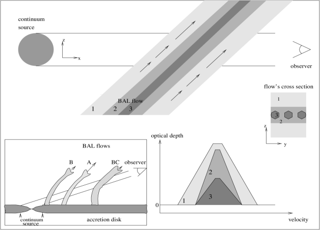
Figure 10: Illustration of the kinematic model. Top sketch shows an accelerating BAL flow crossing the line of sight between the observer and the continuum source, this geometry explains the appearance of stable (velocity-wise) detached troughs seen in most BALQSOs. In PG 0946+301 we postulate the existence of three substrates in the flow: 1. High ionization material with a small total column density per unit velocity [$N(v)$]. 2. High ionization material with large $N(v)$. 3. Low ionization material embedded in substrate 2 but with a smaller covering factor. On the middle right of the figure we show a possible cross section for the flow which assumes that the low ionization material appears in separated flow tubes. This gives the low ionization material smaller covering factor than that of the high ionization material. In the plot at the bottom right of the figure we show the resulting apparent optical depths from this model. Substrate 1 represents the optical depth seen in the O VI and C IV lines, substrate 2 represents the optical depth seen in the S VI and substrate 3 is for the low ionization lines O III, Si IV, N III and C III. The cartoon at the bottom left shows a possible geometry for the entire BAL flow seen in PG 0946+301 (BC: broad component).

Component B is seen in all seven lines and has a well defined profile, therefore we concentrate on constructing a detailed flow model for it. The model is based on the generic BAL flow-model described in Arav (1996). What is seen in the HST data is a wide (velocity-wise; with similar use of the term ‘wide’ hereafter) high-ionization flow that reaches $\tau_{max}\simeq 2-2.5$ at –10100 km s^-1. In the midst of this flow there is a low ionization component which is narrower and although it is probably optically thick, it reaches only $\tau_{max}\simeq 1.1$ (also at –10100 km s^-1). However, to complicate this picture, the high ionization S VI seems to follow the morphology of the low ionization lines but with $\tau_{max}\simeq 2$. The simplest model that is consistent with this phenomenology is of a wide high-ionization flow with a positive gradient of total column density per unit velocity [$N(v)$] toward its center (–10100 km s^-1). We propose that once $N(v)$ is high enough, sub-flows of lower ionization material are forming. The low ionization flows have a lower covering factor than the high-ionization flows, and one can picture them as flow tubes directed along the high ionization flow sheets (see Fig. 4). We invoke the gradient of $N(v)$ in the high-ionization flow in order to explain the absence of a wide S VI component. Since the solar abundance of sulphur is 20 and 50 times lower than those of carbon and oxygen, a larger high-ionization $N(v)$ is needed to detect the S VI line. A larger high-ionization $N(v)$ at the midst of the flow also makes the appearance of low ionization material more plausible. A smaller covering factor for the low ionization flow is necessary once we accept that the low ionization flow is saturated but not as deep as the O VI or S VI flow.

The C IV ground-based observation is of much lower resolution. It shows a well defined component B at the expected velocity position with a FWHM of 800 km s^-1 and $\tau_{max}\simeq 2.3$ (see Fig 2). An 800 km s^-1 FWHM value is between the 1100 km s^-1 FWHM of O VI and the 500 km s^-1 FWHM of the low ionization lines. In the context of the kinematic model, we would expect such a behavior since carbon is less abundant than oxygen (by a factor of 2.4) and since C IV ionization potential is 64 eV compared to 138 eV of O VI.

Another feature that is widest in O VI, less wide in C IV and narrower still in the other lines, is the optical depth rise around –4000 km s^-1. The O VI trough starts rising at –3500 km s^-1 and at –3700 km s^-1 it reaches $\tau=1$ The C IV trough starts rising only around –4000 km s^-1 and reaches $\tau=0.5$ at –4200 km s^-1. All the other BALs (including S VI) have $\tau=0$ between –3800 km s^-1 and –4000 km s^-1. Only beyond –4200 km s^-1 the other lines start having appreciable optical depths. This is consistent with the gradient of $N(v)$ we invoked above and again shows a somewhat wider velocity covering for O VI relative to C IV.

To explain the smaller covering factor observed in the low ionization flow, the model of component B invokes the existence of low ionization flow tubes within the high ionization flow sheets, A prediction of such a model is that stronger variability should be observed in the low ionization lines as the flow tubes move across the line of sight in a keplerian motion. However, this is not the case if the number of flow tubes is large enough to smooth the variability caused by the few flow tubes which are entering or leaving the line of sight.

An alternative explanation for the different covering factors seen in component B can be related to size of continuum emitting region. If the continuum emission arise from an accretion disk, the higher energy photons should come from a smaller hotter part of the disk. Therefore, the shorter wavelength lines in the flow should see a smaller emitting region and thus will have larger covering factors. We reject this alternative since we would expect that the O III line, which sees the hardest continuum of all seven BALs, to have the highest covering factor and thus the largest optical depth. As the data show, this is not the case.

Models for the other flow components are less constrained by the data. However, the main features of component B model are consistent with the data for the other two. In the broad component we again have a wide high ionization flow (seen in O VI, C IV and S VI) in which low ionization sub-flows are embedded (subcomponents C, D and E). Due to the different morphologies, it is plausible that the C IV and S VI absorptions are not saturated, whereas the O VI is. This factor will be significant for ionization and abundances studies of the flow. Higher quality data are needed to verify this assumption and for studying the low ionization subcomponents in detail. It is of course possible that some of the subcomponents C, D, and E are in fact totally separate outflows. Component E has the highest chance of being a separate flow since it is seen in all seven lines and is the lowest velocity feature in the whole flow. In component A only the high ionization flow is present and the non (or marginal) detection of a low ionization component might be correlated with the lower $\tau_{max}(S~{}VI)$ seen in this component compared with $\tau_{max}(S~{}VI)$ seen in Component B.

7 DISCUSSION

7.1 The validity of the integrated column density approach in IEA studies

Almost all attempts to study ionization equilibrium and abundances (IEA) of BAL outflows used apparent integrated ionic column densities ($N_{ion}$) measured from the BALs as the basis of the analysis (Korista et al. 1996; Turnshek et al. 1996; Hamann 1996). It was always stated that these $N_{ion}$ are only lower limits due to the assumption made in their extractions (see discussion in K92), but the severity of the problem was not realized and the IEA studies proceeded on the assumption that the apparent $N_{ion}$ are a good approximation to the real $N_{ion}$. The work presented here demonstrates the inadequacy of this approach and thus strengthens similar conclusions reached by Arav (1997). As shown in § 3.2 there are strong variations in the ratio of apparent $\tau(v)$ in different BALs. This feature suggests that comparing integrated $N_{ion}$ of different lines is misleading and that it is necessary to work with $N(v)_{ion}$ to obtain physically meaningful results. Even more important is the evidence for BAL saturation over parts of their velocity extent (§ 4.1). Although the apparent $\tau_{max}$ in component B only vary by a factor of two between the different BALs, the true optical depth can vary by a much larger factor (even a factor of a hundred cannot be excluded), which is different for each ion. Therefore, saturation and velocity-dependent ionization changes, renders an IEA analysis based on apparent $N_{ion}$ futile and misleading.

How can we use the available data to obtain better constraints on the IEA in PG 0946+301? From the section above it is clear that before any ionization codes can be used we must obtain a reliable determination of real $N(v)_{ion}$. Parts of the flow that are saturated can only tell about the geometry of the flow. On the other hand the broad component (between –9000 and –4500 km s^-1) is probably the least saturated part in most BALs (see § 3.2). We can use the fact that O VI is saturated across the broad component in order to derive more accurate $\tau(v)$ for the other lines. While doing so we must address the possibility that the covering factors of the ions may differ. We can make the assumption that the relative covering factors in the broad component are similar to those seen in component B. This is of course by no means certain, only plausible. Extrapolating from component B we can expect the covering factors of C IV to be most similar to O VI followed by that of S VI. Component B of S VI is only half as wide as the O VI one, but has a similar $\tau_{max}$. In the broad component it seems that the O VI profile is broadest followed by C IV and than S VI. However, this affects only about 1000 km s^-1 interval at the low velocity edge of the flow (between –3500 and –4500 km s^-1) and much less than that at the high velocity edge. Therefore, it is reasonable to assume that between –9000 and –4500 km s^-1 the covering factor of O VI, C IV and S VI are similar. In the low ionization lines the broad component does not appear to be saturated. Therefore, assuming the same covering factor as that of the high ionization lines should not lead to large underestimates of real optical depth.

We note that the available data for the O III $\lambda$702, O IV $\lambda$609, O V $\lambda$630 and N III $\lambda$685 BALs is of too low a quality for IEA studies. It is the combined analysis of high quality data for these lines together with similar data for the longer wavelength CNO BALs that will enable us to substantially improve our understanding of the IEA in this object, and by extension in high ionization BALQSOs in general.

7.2 On the question of meta stable lines

Pettini and Boksenberg (1986) identified the O V^∗ $\lambda$760.4 meta stable line in the IUE spectrum of PG 0946+301. Detection of meta-stable lines is of high interest since these lines can only come from a very high density gas ($n_{e}\mathrel{\raise 1.29167pt\hbox{$>$}\mkern-14.0mu\lower 2.58334pt\hbox{$\sim$}}10^{11}$; see K92 for discussion). Therefore, we checked our better data of PG 0946+301 for the existence of BALs from meta-stable lines. Our upper limit for $\tau$ C III^∗ $\lambda$1175.7 meta-stable line is 0.05. No significant upper limit can be set for the O V^∗ $\lambda$760.4 meta-stable line, since its B component occurs at the midst of the BAL blend (710–785 Å) and at the edge of the G190H data which is of low quality. Within these limits no feature is seen in the data. For N IV^∗ $\lambda$923 meta-stable line the limit is more tricky to asses. The expected position of component B for N IV^∗ $\lambda$923 (892 Å) appears at the edge of an observed absorption feature with $\tau=0.3-0.4$. However, this absorption feature is very probably due to intervening absorption systems. Based on observed Ly$\alpha$ forest lines (see Appendix B) we identify two intervening O VI absorption components within this feature, the red component of one and the blue of the other. The reliability of this identification is strengthened by the appearance of the other doublet component in both systems. Therefore, it is most likely that the observed feature is due to intervening O VI, but a small contribution from N IV^∗ $\lambda$923 cannot be excluded. We conclude that there is no evidence for BALs from meta-stable lines in the HST data of PG 0946+301.

It is possible that the absorption feature that Pettini and Boksenberg (1986) attributed to O V^∗ $\lambda$760.4, might be due to absorption from N IV $\lambda$765 and/or the S IV quadruplet at 750 Å, which were not considered in that work. the IUE data.

7.3 Micro-physics of the Flow

A long standing question concerns the existence and properties of a confining medium for the BAL flow. (Weymann, Turnshek, & Christiansen 1985; Arav & Li 1994, Murray et al. 1995, Weymann 1997). Our current analysis does not shed new light on this question. The flow model we described can be made of either continuous flow components or have these components made of little cloudlets embedded in a confining medium. At first glance cloudlets seems to make the low ionization substrate we invoke unnecessary. The difference in covering factor can arise from the difference in sizes between the low ionization and high ionization region within a given cloudlet. We think this is unlikely however, as such a model requires two forms of fine tuning. First, the need to have just the right distribution of cloudlets to make the $\sim 2/3$ covering factor for the low ionization flow (higher cloudlet concentration will make the covering factor effectively one). Second, a way must be found to avoid different covering factor for each low ionization line, since there is no a-priori reason why inside each cloudlets the optically thick zone for Si IV and C III should coincide. Therefore, it seems more plausible to create the covering factor of the low ionization flow by the global geometrical effect we use.

7.4 The Case for Better Data on PG 0946+301

As described in the Introduction, the suitability of this PG 0946$+$301 for IEA studies makes it the prime target for a multiwavelength campaign. Re-observation of the full rest frame spectral region (400 – 1700 Å) using contemporaneous HST/STIS, FUSE and ground-based spectroscopy will prove crucial to our still developing understanding of this phenomenon. The 8 ionic transitions labeled in Figure 5 as well as the important ones of O IV $\lambda$554 and O III $\lambda$508 will be available for a much better study ($\S$ 3) than we could do using the HST FOS/G160L spectrum. Saturation limits (see § 4.1) can be improved by more than an order of magnitude allowing for a determination of real column densities as function of velocity. The spectral coverage of FUSE contain BALs that can serve as unique saturation diagnostics, enabling us to determine saturation levels up to a hundred times the apparent optical depth, as well as BALs from very high ionization states (Si XII and S XIV). X-ray observations would also prove advantageous in helping to constrain the higher energy ionizing spectrum as well as providing an estimate of the total line of sight column density. Variations in the troughs on time scales of roughly one year have been observed in this object and so these multiwavelength observations would need to be contemporaneous.

Appendix A: Optical depth template extraction

In this appendix we describe in more detail how we extracted the optical depth templates for the ions with non-overlapping BAL troughs that are displayed in figures 2 and 3. Most of these lines (apart from C III) are multiplets, and the observed troughs are a convolution of the function that describes the column density as a function of velocity and the multiplet structure of the line. To probe the structure of the BAL outflow we want to compare the column densities of the different ions as a function of velocity, and a deconvolution procedure has to be applied to the observed BAL troughs. We have experimented with three different methods described below.

A.1 Direct inversion method

The simplest method, which works quite well in most cases, is direct inversion. After the continuum is determined as described in section 4.2, the spectrum is first normalized to a continuum level of one for all wavelengths. We then take a region of the spectrum that contains the BAL trough considered, and extends by at least the width of the multiplet beyond the region where absorption due to the ion is thought to be present. This part of the spectrum is then rebinned to a new wavelength grid that is equidistant in $\log(\lambda$), and has a bin separation close to the original one with the constraint that the separation between the two strongest components of the multiplet corresponds to an integer number of bins. The logarithmic grid has the advantage that the separation of the different multiplet components remains the same number of bins as the multiplet is Doppler-shifted. Since our original spectrum is highly oversampled the rebinning does not degrade the spectrum significantly.

Now consider the most simple case of a doublet. We first define the following symbols:

• $n$ is the total number of points in the fitted spectrum

• $s$ is the number of bins corresponding to the doublet separation

• $w_{i}$ ($1\leq i\leq n$) is the wavelength of a gridpoint on the logarithmic grid

• $f_{i}$ is the normalized flux at $w_{i}$

• $v_{i}$ is the velocity that shifts component 1 of the doublet from rest to the wavelength $w_{i}$, and component 2 to $w_{i+s}$

• $\tau_{k,i}$ ($k=1,2$) is the Sobolev optical depth in component k of the multiplet due to the column density of the ion at velocity $v_{i}$:

  $$\tau_{k,i}={{\pi e^{2}}\over{m_{e}c}}g_{l}f_{lu}\lambda{d({{N_{l}}/{g_{l}}})\over{dv}},$$ (A.1)

  where in order to avoid confusion with the algebraic indices we use the notation $g_{l}f_{lu}$ instead of $g_{i}f_{ik}$.

• $\tau_{i}$ is the total optical depth at $w_{i}$

Using these definitions and equation A1, we can now write down the following equation for $\tau_{i}$:

$$\tau_{i}\ =\ \tau_{1,i}\ +\ \tau_{2,i-s}\ =\ \tau_{1,i}+\ {{(g_{l}f_{lu})_{2}}\over{(g_{l}f_{lu})_{1}}}\tau_{1,i-s}\quad$$

as long as we can assume that the population of the lower levels is proportional to their statistical weights. Repeating this for all $v_{i}$ yields a set of coupled linear equations that we can solve for $\tau_{1,i}$, for a given vector $\tau_{i}=-\ln(f_{i})$. The set of equations can be written symbolically as $\rm{\bf A}\ \cdot{\bf\tau}_{1}=-\ln({\bf f})$, where A has non-zero elements only on the main diagonal (equal to 1) and on the subdiagonal $s$ elements down from the main diagonal (equal to $(g_{l}f_{lu})_{2}/(g_{l}f_{lu})_{1}$).

It is obvious that this method can easily be generalized to multiplets with an arbitrary number of components. The resulting sets of linear equations will have a non-zero diagonal for each component of the multiplet, filled with the constant value ${{(g_{l}f_{lu})_{k}}/(g_{l}f_{lu})_{1}}$, and shifted down or up from the main diagonal by a number of elements equal to the number of wavelength bins that corresponds to the difference in wavelength between component 1 and component k. Even for a large number of points in the spectrum the set of linear equations can be solved fast and efficiently by the use of a banded matrix linear equation solver.

A.2 Regularization methods

Since we are solving for the same number of variables as there are equations, the direct method forces an exact solution, i.e. the fitted spectrum is identical to the observed one. This is not always a desirable property, since for various reasons (very significant noise, or partial covering effects that influence the doublet ratio) the observed spectrum does not behave exactly as our theoretical model assumes. Requiring an exact match with the given doublet ratio can lead to instability and oscillating solutions. This effect is not serious as long as one component of the multiplet has a significantly higher $g_{l}f_{lu}$ value than the others, since in this case the oscillations caused by features in the spectrum that do not follow the expected line ratio model exactly are damped, and die out quickly.

To see this, consider what happens when we try to fit a single strong line with a doublet model. To get the correct optical depth, the fitting procedure will put the strongest line of the doublet at the position of this line. It then expects another absorption line at the position of the other doublet component, but there is none in the data. To compensate for the absorption implied by fitting the single line, the method will then assume negative optical depth in the strongest doublet component at this wavelength. This in turn predicts emission at the position of the other doublet line, and an oscillation sets in. When the $g_{l}f_{lu}$ value of the primary component is much larger than that of the secondary, the oscillation will be damped since each correction is smaller than the previous one by a factor equal to the ratio of the $g_{l}f_{lu}$ values. Otherwise, the oscillations will extend over the entire wavelength range. Thus, this method can cause problems when extracting column density templates in the case that the multiplet components have comparable $g_{l}f_{lu}$ values.

However, since there are physically reasonable models that could lead to equal “effective” optical depth in each component of the multiplet, such as the case in which the line depth is caused by very optically thick clouds that cover the source only partly, it is interesting to extract templates under this assumptions. We have experimented with two methods to stabilize the solution.

The first is the linear regularization technique described in Press et al. (1992). For details we refer to this reference, but the basic idea is that one does not minimize the difference between the fit and the model alone (i.e. solve the equation $\rm{\bf A}\ \cdot{\bf\tau}_{1}=-\ln{\bf f}$), but rather attempts to find the best fitting solution while also getting as close as possible to some a priori constraint, for instance that the solution should be relatively smooth. As derived in Press et al., this leads to a set of linear equations of the form

$$\rm({\bf A}^{T}\ \cdot{\bf A}\ +\ \lambda{\bf H})\cdot{\bf\tau}_{1}=-{\bf A}^{T}\cdot\ln{\bf f}$$ (A.2)

in which the matrix H describes the a priori constraint, and the parameter $\lambda$ allows a trade-off between fitting as close as possible to the original equation ($\lambda=0$) or to the constraint ($\lambda>>1$). We experimented with the form of H, and found good regularization for the choice $h_{i,i}=4$, $h_{i-1,i}=-1$, $h_{i-2,i}=-1$, $h_{i+1,i}=-1$, $h_{i+2,i}=-1$ and all other elements equal to zero. For $\lambda$ we used the value 0.5.

The second method we tried was modeling the $\tau_{1,i}$ distribution by a large number of gaussians with a width comparable to the resolution, i.e. about 4 datapoints. Each gaussian in the primary component of the multiplet implies similar gaussians at the wavelengths corresponding to the other multiplet lines, the amplitudes again being proportional to the $g_{l}f_{lu}$ values. We then used a least squares method based on singular value decomposition to obtain the optical depths of the primary multiplet component that best fit the spectrum.

In figure 11 we plot the results of an extraction of the column density profile for the C IV line under the assumption that the doublet ratio is 1 instead of 0.5 . Clearly the direct method is unstable, and unusable for this profile. The method of Gaussian fits damps out a lot of the instability, but still shows a considerable amount of oscillation at the doublet separation. The regularization method performs best, yielding a column density distribution without negative excursions, and relatively little oscillation. It should be noted however that the regularization does involve smoothing and loss off information.

Figure 11: The results of applying three different deconvolution methods to the observed line profile of C IV, under the assumption that the effective doublet ratio is 1. Both direct inversion and multiple Gaussian fitting introduce oscillations, only the regularization method gives physically acceptable results.

The three methods were also tested by applying them to simulated line profiles with added noise or constructed with the wrong line ratios. The direct method was found to perform best since it does not manipulate the original data. However, it is most likely to introduce oscillations if the line ratios are wrong. The regularization is the best for avoiding the instability associated with equal strength components and noise. We found that the gaussian fitting method is good at suppressing the noise while still showing oscillations if the line ratios are incorrect, which is a useful diagnostic tool.

A.3 Noise and spurious features

Figure 12: This figure illustrates the expected level of fluctuations in the deconvolved profiles of optical depth as a function velocity due to noise in the observations. A smooth underlying optical depth profile (the thin line in the figure) was used to generate an absorption line profile, which was then degraded to a signal to noise level corresponding to the ones for O VI, C IV and Si IV. The resulting line profile was then deconvolved using direct inversion, just as it was done for the real profiles in Figure 2. Features in the real profile comparable or smaller than those present in the simulation shown here are not significant.

To estimate what features in the extracted templates are real and which ones are likely to be due to noise, we extracted templates from artificial spectra that were realizations (with a realistic signal to noise ratio) of a smooth spectrum similar in shape to the observed one. The results for O VI, C IV and Si IV are plotted in figure 12, which can be compared with the real spectra in Figure 2. For these lines, the S/N ratios in the continuum are about 18, 45 and 24 respectively. From this comparison e conclude that in the broad component the O VI profile does not contain measurable substructure, but that the substructures in the C IV and Si IV templates are significant.

Even if structures are significant, they need not necessarily be reflections of features in the column density distribution, since there are also other effects apart from noise that could influence the templates, such as lines of other species, or components that are optically thick but partially covering the source and thus do not fit the assumed multiplet structure. A good example of this is the C IV template for a doublet ratio of one obtained by the Gaussian fitting method in figure 11. However, moderate departures from the theoretical line ratios (say 0.7 instead of 0.5) do not lead to large apparent substructures.

APPENDIX B: INTERVENING ABSORPTION

As in all quasars, absorption features from intervening material are also seen in the spectrum of PG 0946+301. In this appendix we attempt to catalogue the intervening absorption features in order to avoid confusion with BAL features, facilitate future studies of this object, and account for all the absorption features seen in the spectrum.

B.1 Ly$\alpha$ systems

We identify 14 suspected Ly$\alpha$ absorption systems. Three of these (5, 9 and 10) are clearly seen in other lines and two more might be seen in Ly$\beta$ (7 and 12). Observed wavelength and equivalent widths for the Ly$\alpha$ systems are given in Table 3. We note that system 1 might be a BAL feature associated with component B of Si III $\lambda$1206.5 but we classify it as an intervening Ly$\alpha$ absorption since it is significantly narrower than other BAL features associated with component B. Also, Ly$\alpha$ lines 4 and 8 are quite marginal with the available S/N.

In Table 3 we also give a subjective assessment for the reality of absorption features that can arise from other lines associated with each intervening Ly$\alpha$ line. It is interesting to notice how much of the non-BAL absorption features around 1920–1980 Å can be explained by lines associated with the Ly$\alpha$ systems (see figure 13). In particularly system 10 has a strong Ly$\beta$ and O VI lines in that region (and also a clear C IV doublet). The most intriguing is system 9, which is too broad too be a simple Ly$\alpha$ forest line. Some of the absorption features that can be explained by system 10 around 1960–1990 Å can also arise from system 9. Furthermore, the absorption feature at 840 Å (rest frame, see Fig. 5) is consistent with being the Ly$\gamma$ of system 9. However, system 9 doesn’t have a definite C IV component, although it might be somewhat obscured by the edge of the Si IV BAL. System 5 is clearly seen in C III, C IV, and may be seen in O VI. C IV absorption associated with system 10 appears at the high velocity edge of the Si IV BAL and should not be confused as being a part of it. We do not find N V or Si IV lines associated with any of the Ly$\alpha$ systems.

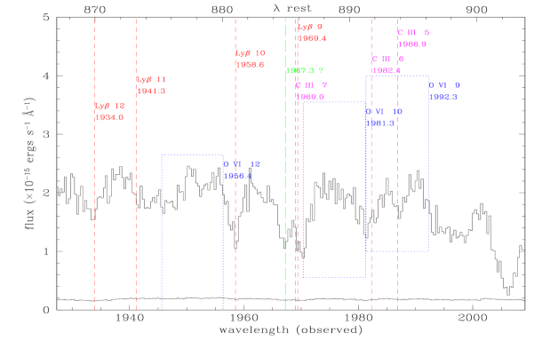
Figure 13: Segment of PG 0946+301 spectrum with intervening absorption marked. Vertical lines designate the calculated positions of metal lines and Ly$\beta$, which correspond to identified Ly$\alpha$ systems (see table 3). Ly$\beta$ and C III lines are marked with dashed lines. The ion and the number of the system is written just to the right of the line and its calculated wavelength is written underneath. The O VI doublets are marked with a rectangular dotted box where the vertical sides correspond to the positions of the doublet components. The label of the system and the calculated wavelength of the red component are attached to the right of the component. To avoid cluttering we omitted most of the non detected lines. About 75% of the absorption features seen in this part of the spectrum can be identified with lines associated with known Ly$\alpha$ intervening systems. Absorption seen longward of 1990 Å is part of the S VI BAL.

B.2 Galactic Lines

A strong Mg II doublet ($\lambda\lambda$2796.35, 2803.32) is seen in the observed frame and we used it to calibrate the the observed wavelengths. Two systems of galactic Fe II absorption lines at almost zero redshift are seen in the spectrum. Working in the frame where the observed galactic Mg II is at zero velocity, we find that observed absorption features are matching well with Fe II lines (2344.21, 2374.46 and 2382.76 Å) The second identified system is the two Fe II zero energy level transitions at 2586.65 and 2600.17 Å. The absence of other components of the Fe II multiplets is explained by noticing that all these components are not truly ground state transitions, but arise from slightly higher energy states.

B.3 Unidentified Lines

Very few absorption features in the spectrum are left unexplained once the BAL absorption and the different intervening systems are accounted for. The feature at 1967.3 Å is probably another Ly$\alpha$ forest line. The absorption features seen at 2138 Å and 2177.4 Å are part of the BAL flow. They match component E of the flow in C III and N III respectively. We identified this component (the lowest velocity one) in all 7 BALs for which we have an optical depth solution. The very broad feature at 2305.9 Å should be a BAL feature. There is a very good agreement with the expected position of a S IV BAL, but this is a relatively weak line and its stronger brothers to the blue should be much deeper. As noted in § 5.7, this is one of the most puzzling issues in the BAL features of this object

Table 3: Intervening lines
no.	$\lambda$(Ly$\alpha$)	EW(Ly$\alpha$)	Ly$\beta$	C III	C IVb	C IVr	O VIb	O VIr
	(obs)	(rest)
1	2592.7	0.20	0	0	1b	0b	0b	0b
2	2517.5	0.24	1b	0	0	0	1b	0
3	2514.9	0.23	1b	0	0	0	0	0
4	2494.9	0.10	1	0b	1	1	0	0
5	2472.2	0.48	1	3	3	3	2	1b
6	2466.6	0.37	1	2b	1	1	0	1
7	2450.0	0.32	2b	0b	0	1	1	2
8	2351.9	0.15	0	0	0	0b	0b	0b
9	2334.2	1.65	2b	0	1	1	3	2b
10	2321.3	0.82	3	1	3	3	3	3
11	2300.8	0.14	1	0	0	0	1	1
12	2292.1	0.52	2	0	0	0	1	1
13	2283.9	0.29	0	0	0	0	0	0
14	2153.2	0.44	1	0	0	0	1	2b

Column 1 gives the number the system, column 2 the observed wavelength of the Ly$\alpha$  line and column 3 gives its rest equivalent width. In columns 4–9 we give a qualitative assessment for the existence of an absorption feature in other lines from the same system. Our key is as follows: 0 - no feature, 1 - marginal, 2 - an absorption feature exists but it either not strong enough for an unambiguous identification or its position does not precisely match the expected one, 3 unambiguous detection at the expected position and with a similar profile. The letter b designate a feature blended with other absorption (mostly BAL but not always). For C IV and O VI the subscript designate the red or blue component of the doublet.

References

- (1) Arav, N., & Li, Z. Y. 1994, ApJ, 427, 700
- (2) Arav, N., Li, Z. Y., & Begelman, M. C. 1994, ApJ, 432, 62
- (3) Arav, N., Korista, T. K., Barlow, T. A., & Begelman, M. C. 1995, Nature, 376, 576
- (4) Arav, N., 1996, ApJ, 465, 617
- (5) Arav, N., 1997 in Mass Ejection from AGN, ASP Conference Series, Vol. 128, ed. N. Arav, I. Shlosman, and R. J. Weymann, p. 208
- (6) Barlow, T. A., in Mass Ejection from AGN, ASP Conference Series, Vol. 128, ed. N. Arav, I. Shlosman, and R. J. Weymann, p. 13
- (7) Barlow, T. A. & Junkkarinen, V. T. 1994, BAAS, 26, 1339
- (8) Cohen, M. H., Ogle, P. M., Tran, H. D., Vermeulen, R. C., Miller, J. S., Goodrich, R. W., & Martel, A. R. 1995, ApJ, 448, L77
- (9) de Kool, M., & Begelman, M.C 1995, ApJ, 455, 448
- (10) de Kool, M., 1997 in Mass Ejection from AGN, ASP Conference Series, Vol. 128, ed. N. Arav, I. Shlosman, and R. J. Weymann, p. 233
- (11) Foltz, C. B., Chafee, F. H., Hewett, P. C., Weymann, R. J., & Morris, S. L. 1990, BAAS, 2, 806
- (12) Foltz, C. B., Weymann, R. J., Morris, S. L., & Turnshek, D. A. 1987, ApJ, 317, 450
- (13) Foltz, C. B., Wilkes, B., Weymann, R. J., & Turnshek, D. A. 1983, PASP, 95, 341
- (14) Grillmair, C.J., & Turnshek, D.A. 1987, poster paper from the QSO Absorption Lines: Probing the Universe conference
- (15) Hamann, F. 1996, ApJS, 109, 279
- (16) Hamann, F., Korista, T. K., & Morris, S. L. 1993 ApJ, 415, 541
- (17) Hamann, F., Barlow, T. A., Junkkarinen, V. T., & Burbidge, E. M. 1997, ApJ, 478, 80.
- (18) Korista, K.T., Weymann, R.J., Morris, S.L., Kopko, M., Turnshek, D.A., Hartig, G.F., Foltz, C.B., Burbidge, E.M., & Junkkarinen, V.T. 1992, ApJ, 401, 529
- (19) Korista, T. K., Voit, G. M., Morris, S. L., & Weymann, R. J. 1993, ApJS, 88, 357
- (20) Korista, T. K., Hamann, F., Ferguson, J., & Ferland, G. J. 1996, ApJ, 461, 645
- (21) Junkkarinen, V.T., Beaver, E.A., Burbidge, E.M., Cohen, R.D., Hamann, F., & Lyons, R. W., 1997, in Mass Ejection from AGN, ASP Conference Series, Vol. 128, ed. N. Arav, I. Shlosman, and R. J. Weymann, p. 220
- (22) Junkkarinen, V.T. et al. 1998, in preparation
- (23) Junkkarinen, V.T., Burbidge, E.M. & Smith, H.E 1983, ApJ, 265, 51
- (24) Mathur, S., Wilkes, B.J., Elvis, M.S., & Fiore, F. 1994, ApJ,434, 493
- (25) Mathur, S., Wilkes, B.J., & Aldcroft, T. 1997, ApJ, 478, 182
- (26) Morton, D.C. 1991, ApJS, 77, 119
- (27) Murray, N., Chiang, J., Grossman, S.A., & Voit, G.M. 1995, ApJ, 451, 498
- (28) Murray, N., & Chiang,J. 1995, ApJ, 454, L105
- (29) Ogle, P. M., 1997 in Mass Ejection from AGN, ASP Conference Series, Vol. 128, ed. N. Arav, I. Shlosman, and R. J. Weymann, p. 78
- (30) Press, W.H., Teukolsky, S.A., Vetterling, W.T., & Flannery, B.P. 1992, Numerical Recipes: The Art of Scientific Computing, Second Edition (Cambridge: Cambridge University Press)
- (31) Pettini, M. & Boksenberg, A., in ESA Proceedings of an International Symposium on New Insights in Astrophysics. Eight Years of UV Astronomy with IUE, p 627
- (32) Seaton, M.J. 1992, Rev. Mex. Astron. Astrofis., 23, 19
- (33) Telfer, R.C., Kriss, G.A., Zheng, W., Davidson, A.F., & Green, R.F. 1998, ApJ, in press
- (34) Turnshek, D. A. 1988, in Space Telescope Sci. Inst. Symp. 2, QSO Absorption Lines: Probing the Universe, ed. S. C. Blades, D. A. Turnshek, & C. A. Norman (Cambridge: Cambridge Univ. Press), 17
- (35) Turnshek, D. A., et al. 1996, ApJ, 463, 110
- (36) Verner, D.A., Barthel, P.D., & Tytler, D. 1994, A&AS, 108, 287
- (37) Verner, D.A., Verner, E.M., & Ferland, G.J. 1996, Atomic Data & Nuclear Data Tables, 64, 1
- (38) Weymann, R. J., Turnshek, D. A., & Christiansen, W. A. 1985, in Astrophysics of Active Galaxies and Quasi-stellar Objects, ed. J. Miller (Oxford: Oxford Univ. Press) 333
- (39) Weymann, R. J., Morris, S. L., Foltz, C. B., & Hewett, P. C. 1991, ApJ, 373, 23
- (40) Weymann, R. J., in Mass Ejection from AGN, ASP Conference Series, Vol. 128, ed. N. Arav, I. Shlosman, and R. J. Weymann, p. 3
- (41) Wilkes, B.J., 1985, ApJ, 288, L1.