Dynamical models of NGC 3115

Abstract

We present new dynamical models of the S0 galaxy N3115, making use of the available published photometry and kinematics as well as of two-dimensional TIGER spectrography.

The models are based on a detailed model of the luminosity distribution built using an MGE fit on HST/WFPC2 and ground-based photometric data. We first examined the kinematics in the central $40\arcsec$ in the light of two-integral $f(E,J)$ models. Jeans equations were used to constrain the mass to light ratio, and the central dark mass whose existence was suggested by previous studies. The even part of the distribution function was then retrieved via the Hunter & Qian formalism. We thus confirmed that the velocity and dispersion profiles in the central region could be well fit with a two-integral model, given the presence of a central dark mass of $\sim 10^{9}$ $\mbox{M}_{\sun}$. However, no two-integral model could fit the $h_{3}$ profile around a radius of about $25\arcsec$ where the outer disc dominates the surface brightness distribution.

Three integral analytical models were therefore built using a Quadratic Programming technique. These models showed that three integral components do indeed provide a reasonable fit to the kinematics, including the higher Gauss-Hermite moments. Again, models without a central dark mass failed to reproduce the observed kinematics in the central arcseconds. This clearly supports the presence of a nuclear black hole of at least $6.5\times 10^{8}$ $\mbox{M}_{\sun}$in the centre of NGC 3115. These models were finally used to estimate the importance of the dark matter in the outer part of NGC 3115, suggested by the flat stellar rotation curve observed by Capaccioli et al. (1993).

This study finally points out the difficulty of integrating independently published data in a coherent and consistent way, thus demonstrating the importance of taking into account the details of the instrumental setup and the reduction processes.

1 Introduction

Early-type disc galaxies pose a specific problem for dynamical modeling as neither the bulge nor the disc can be neglected in the computation of the gravitational potential. First, it is generally difficult to disentangle the photometric components according to a priori fixed criteria such as the ellipticity or surface brightness profiles. Although there exists different methods to build corresponding realistic photometric models, they are usually limited to two component systems (e.g. disc plus spheroid, Byun & Freeman 1995) which do often not reflect the true morphology of the galaxy. Then, the different internal dynamics of each component has to be taken into account. Asymetrical Line Of Sight Velocity Distributions (LOSVDs) observed in discy ellipticals (e.g. Scorza & Bender 1995) confirmed the fact that the classically measured velocity $V$ and dispersion $\sigma$ do not sufficiently constrain their dynamical structure. Because of these difficulties, the analysis is usually restricted to the central region, or to regions where one component dominates the light (e.g. Jarvis & Freeman 1985).

A number of techniques to build realistic distribution functions of such complex objects have recently been developed. Hunter & Qian (1993) proposed a viable scheme to retrieve the even part of the axisymmetric two integral distribution function corresponding to a given mass model. It was used by van den Bosch & de Zeeuw (1996) for a set of models including a spheroid and a disc. In principle, this method can be applied to more complex potentials: this will be demonstrated in the present paper. As a further step, three integral axisymmetric models can be built, using for example the Schwarzschild method in which one derives the best combination of orbits constrained to fit a set of observational data (e.g. van der Marel et al. 1998, Cretton & van den Bosch 1998). In this paper, we wish to present the application of another technique, namely Quadratic Programming (Dejonghe 1989)

NGC 3115 is interesting in many different aspects. First it has long been assumed to be the prototype of the S0 galaxy type: a bulge dominated galaxy with an embedded disc and very little gas and dust. With a distance of about 10 Mpc and a nearly edge-on inclination, NGC 3115 is also a perfect target for optical observations. Numerous studies were focused on the understanding of its morphology and kinematics. NGC 3115 contains a double disc structure with an outer Freeman type II disc extending up to $\sim 140\arcsec$ and a nuclear disc (inside $3\arcsec$) clearly revealed by the HST/WFPC2 pictures (Kormendy et al. 1996). Its outer disc was found to exhibit a weak spiral arm structure (Capaccioli et al. 1987, Silva et al. 1988) and to thicken outwards (Capaccioli et al. 1988). The spheroidal component does not seem to follow the classical $r^{1/4}$ law, and the flattened halo of NGC 3115 extends up to $20\arcmin$ (Capaccioli et al. 1987).

The kinematics of NGC 3115 also deserved a complete survey: Illingworth & Schechter (1982) presented an extensive series of spectroscopic observations demonstrating that the bulge of this galaxy was nearly consistent with being an isotropic rotator. NGC 3115 has also been one of the best candidates for the presence of a central dark mass since the spectroscopic observations of Kormendy & Richstone (1992): spherical models suggested an increase of $M/L$ by more than a factor of 10 inside $2\arcsec$, which is difficult to account for with normal stellar populations. This conclusion was based on the observed velocity gradient and central gaussian velocity dispersion $\sigma_{0}$, the latter nearly reaching 300 $\mbox{km.s}^{-1}$at a resolution of $\sim 1\arcsec$ FWHM. This trend has been very recently confirmed with FOS spectroscopy (Kormendy et al. 1996), yielding $\sigma_{0}\sim 445$ $\mbox{km.s}^{-1}$at HST resolution. Other studies mainly focused on the major-axis kinematics (Carter & Jenkins 1993, van der Marel et al. 1994, Bender et al. 1994, Fisher 1997). Finally Capaccioli et al. (1993) have shown that the stellar rotation and dispersion profiles were flat at large radii ($R>100\arcsec$), thus indicating the presence of a massive dark halo.

In this paper, our aim is to make detailed models of this early type disc galaxy, e.g. constrain its distribution function, fully taking into account the available published data. This includes, for the first time, two-dimensional spectroscopic observations. In Sect. 2 we describe the photometry and spectroscopic observations used for the modeling, including new HRCAM images, the WFPC2 $V$ band image as well as original TIGER spectrography of the central region. The photometric models based on the MGE formalism are presented in Sect. 3 and their corresponding dynamical Jeans models in Sect. 4. Numerical two integral distribution functions are derived using the Hunter & Qian method and analysed in Sect. 5. Two and three integral models are computed in Sect. 6 with the help of the Quadratic Programming method. Conclusions are drawn in Sect. 7.

2 Observational data

2.1 Photometry

Dynamical modeling first implies the availability of a luminosity model. This requires images with high resolution to get details on the central region, but also with a large field of view to correctly sample the line-of-sight at large radii. A wide field $V$ band image, obtained with a focal reducer on the 1.23m telescope at Calar Alto, was kindly put at our disposal by Cecilia Scorza. We then retrieved the $V$ band WFPC2 image (F555W) of NGC 3115 from the HST archives at ECF (PI Faber). We finally used a $V$ band image obtained by Jean-Luc Nieto in April 1992 with HRCAM at the CFHT. All these images were reduced and normalized using aperture photometry available in the literature (Poulain 1986 & 1988, de Vaucouleurs & Longo 1988). These calibrations led to individual errors smaller than 0.05 $\mbox{mag.arcsec}^{-2}$with an excellent overall agreement. The characteristics of the different images are given in Table 1.

Table 1: Characteristics of the $V$ band images of NGC 3115.

	Calar Alto	HRCAM	WFPC2
pixel size	$1\aas@@fstack{\prime\prime}55$	$0\aas@@fstack{\prime\prime}11$	$0\aas@@fstack{\prime\prime}0455$
seeing ($\sigma_{\star}$)	$\sim 3\arcsec$	$0\aas@@fstack{\prime\prime}7$	-
field of view	$10\arcmin\times 15\arcmin$	$70\arcsec\times 110\arcsec$	$34\arcsec\times 33\arcsec$
exp. time	240s	120s	1030s
airmass	1.65	1.13	–

2.2 Spectroscopy and kinematics

2.2.1 TIGER data

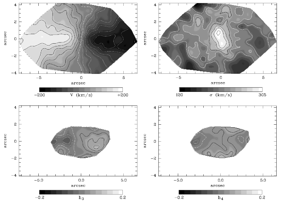
Figure 1: TIGER stellar kinematical maps: velocity (top left), dispersion (top right), $h_{3}$ (bottom left) and $h_{4}$ (bottom right). The isocontour step is 25 $\mbox{km.s}^{-1}$for both $V$ and $\sigma$, and 0.05 for $h_{3}$ and $h_{4}$.

Figure 2: Comparison between the different published kinematics and the TIGER 1992 data. Each symbol corresponds to a reference as shown in the $V$ panel. F97 = Fisher 1997; vdM = van der Marel et al. 1994 (WHT data only); BSG = Bender et al. 1994; KR = Kormendy & Richstone 1992 (exposures 29F48, 29F42, 34F16; see KR92); CJ = Carter & Jenkins 1993.

We observed NGC 3115 with the TIGER integral field spectrograph (Bacon et al. 1995) at the CFHT in April 1992 and subsequently in April 1996. The lens diameter was set to $0\aas@@fstack{\prime\prime}39$ and the spectral domain to 5130–5520 Å for both runs. The spectra were extracted and calibrated in the standard way using the TIGER software written at the Lyon Observatory. This includes bias subtraction, flat-fielding, spectra extraction, wavelength calibration, cosmic rays removal and differential refraction correction (see Emsellem et al. 1996 for more details). The individual exposures were then accurately centred and merged. Variations in the overall atmospheric transparency were smaller than 1% and corrected. We thus obtained one set of spectra for each run, consisting of 624 and 391 spectra for the run92 and run96 respectively. The final seeing of each data cube was estimated a posteriori by comparing images reconstructed from the spectra with the $V$ band WFPC2 image. Details on the characteristics of both sets of data are given in Table 2. Note that although the set of data obtained in April 1996 has a significantly better spatial and spectral resolution, we will mainly present the data set obtained in April 1992 as the signal to noise is higher and the field of view larger.

Table 2: Observational characteristics of the TIGER spectrographic exposures. The fields of view are only indicative as the coverage of the merged TIGER spectra are not rectangular. All individual frames had an exposure time of 30 mn.

	1992 Run	1996 Run
Lens diam.	$0\aas@@fstack{\prime\prime}39$	$0\aas@@fstack{\prime\prime}39$
Field of view	$14\aas@@fstack{\prime\prime}5\times 7\aas@@fstack{\prime\prime}9$	$7\aas@@fstack{\prime\prime}9\times 7\aas@@fstack{\prime\prime}9$
# of exposures	4	2
# of spectra	624	391
Spect. sampling	1.8 Å .$\mbox{pixel}^{-1}$	1.5 Å .$\mbox{pixel}^{-1}$
Spect. resolution	3.7 Å (FWHM)	3.2 Å (FWHM)
Instr. broadening ($\sigma$)	94 $\mbox{km.s}^{-1}$	78 $\mbox{km.s}^{-1}$
Spect. domain	5130 - 5520 Å	5130 - 5520 Å
Seeing (FWHM)	$1\aas@@fstack{\prime\prime}24$	$0\aas@@fstack{\prime\prime}8$
Stellar templates	$\eta$ Cygni	HR 127065
	K0III	K0III

In order to determine the stellar kinematics we also obtained exposures of a few stellar templates: mainly K giants for run92 and G, K and M giants for run96. All spectra were logarithmically rebinned, the stellar continuum was approximated using a fifth degree polynomial and subtracted. We then derived the 2D kinematics of the central region of NGC 3115 using the FCQ algorithm (Bender 1990) and an optimal template built with the available stellar spectra. This provides the full LOSVD for each spatial element. The LOSVDs were then parametrized with the Gauss-Hermite functions. True moments were also estimated from the positive part of the parametrized LOSVDs (see Emsellem et al. 1996). The results were found to be rather insensitive to the choice of the template, so we decided to use the spectrum of a single K0 giant for both runs. We finally built the maps for each kinematical quantity: $V$, $\sigma$, $h_{3}$ and $h_{4}$ which correspond to the Gauss-Hermite parametrization as well as the estimations of the four first true moments of the LOSVD $\tilde{V}$, $\tilde{\sigma}$, the skewness and the kurtosis.

The mean velocity, velocity dispersion (gaussian fit), $h_{3}$ and $h_{4}$ two-dimensional maps are presented in Fig. 1 (run92). We detect a slight tilt of $10\degr$ of the velocity minor-axis in the 1992 data. The low signal to noise of the new TIGER data set prevented us to confirm this: it would therefore be useful to obtain new high spatial resolution kinematical data along the minor-axis. Note that the $h_{3}$ and $h_{4}$ maps only include spectra with a signal to noise higher than 20.

2.2.2 Comparison with published kinematics

All kinematical data available were compiled, and the FOS/HST ($0\aas@@fstack{\prime\prime}21$ square aperture) and SIS/CFHT data obtained by Kormendy et al. (1996) scanned. As emphasized by different authors (e.g. van der Marel et al. 1994) the gaussian velocity $V$ and dispersion $\sigma$ are not always good estimations of the true $\tilde{V}$ and $\tilde{\sigma}$ moments. This is particularly important in the case of NGC 3115 where high values of $h_{3}$ have been measured (e.g. van der Marel et al. 1994). Therefore, we mainly focused on the data sets including higher order moments of the LOSVDs: van der Marel et al. (1994, hereafter vdM+94), Bender et al. (1994, hereafter B+94), Fisher (1997, hereafter F97) and the TIGER data. In these cases, we used the Gauss-Hermite expansion of the LOSVDs to estimate $\tilde{V}$ and $\tilde{\sigma}$ using the same method as used by Emsellem et al. (1996). Still we made use of other published kinematics such as Kormendy & Richstone (1992, hereafter KR92), Carter & Jenkins (1993), and the recent high spatial resolution FOS/HST and SIS/CFHT data (Kormendy et al. 1996, hereafter K+96). We finally included the data of Illingworth & Schechter (1982, hereafter IS82) for offset axes and of Capaccioli et al. (1993, hereafter C+93) for the kinematics at large radii along the major-axis. The characteristics of each data set are given in Table 3.

Table 3: Observational characteristics of the kinematical (long-slit) data used in this paper (for the FOS/HST data, see Kormendy et al. 1996).

Ref.	slit width	$\sigma_{v}$	seeing (FWHM)	$h_{3},h_{4}$
Illingworth & Schechter 1982	$2$–$3\arcsec$	$100$–$130$ $\mbox{km.s}^{-1}$	$1\aas@@fstack{\prime\prime}5$–$5\arcsec$	no
Capaccioli et al. 1993	$1$–$1\aas@@fstack{\prime\prime}6$	$\sim 40$ $\mbox{km.s}^{-1}$	$>1\aas@@fstack{\prime\prime}5$	no
Kormendy & Richstone 1992	$0\aas@@fstack{\prime\prime}5$	$68$ $\mbox{km.s}^{-1}$	$1\arcsec$–$1\aas@@fstack{\prime\prime}6$	no
Carter & Jenkins 1993	$0\aas@@fstack{\prime\prime}45$	$10$ $\mbox{km.s}^{-1}$	$0\aas@@fstack{\prime\prime}8$	no
van der Marel et al. 1994	$1\arcsec$	$38$ $\mbox{km.s}^{-1}$	$0\aas@@fstack{\prime\prime}96$	yes
Bender et al. 1994	$2\aas@@fstack{\prime\prime}1$	$46$ $\mbox{km.s}^{-1}$	$1$–$2\aas@@fstack{\prime\prime}5$	yes
Fisher 1997	$2\arcsec$	$75$ $\mbox{km.s}^{-1}$	$>1\aas@@fstack{\prime\prime}5$	yes
Kormendy et al. 1996	$0\aas@@fstack{\prime\prime}26$	$\sim 35$ $\mbox{km.s}^{-1}$	$0\aas@@fstack{\prime\prime}57$	-

In Fig. 2, we compare the TIGER kinematics along the major-axis with the ground-based data with similar resolution: they are all in good agreement. The error bars of the TIGER data were determined by the statistics on the fluctuations inside a spatial resolution element, here taken as the FWHM of the PSF. As it turns out, this defines a beam containing on average 7 spectra.

2.3 Convolution and pixel integration

The comparison between observed kinematics and theoretical models requires to take into account the observational characteristics. The seeing smearing and pixel binning have been computed through a double quadrature (see Appendix A). All the comparisons presented in the following sections include this processing, according to the parameters of the relevant data set as tabulated in Table 3. Note that the PSF of the FOS data was derived using an approximation as given in van der Marel et al. (1997).

2.4 Uncertainties in the kinematics

Additional factors linked with the instrumental setup or the data reduction processes can significantly influence the measured kinematics, and in particular the higher order Gauss-Hermite moments. Firstly, an error in the centering or position angle of the slit induces a change in the observed kinematics. In the case of NGC 3115, an offset of $\Delta\alpha=2\degr$ (major-axis) in the position angle of the slit gives $\Delta h_{3}\sim 10$% at $R=35\arcsec$, while the change in velocity amounts to only about 3%. It is also important to control the spectral filtering applied for the retrieval of the LOSVDs as it could lead to underestimate the higher order moments. Finally, the obtained kinematics may be sensitive to the method used (e.g. Fourier fitting, FCQ, etc). In the following paragraph, we discuss such an effect on the central FOS LOSVD.

2.4.1 The central $h_{4}$ value

The central observed FOS LOSVD is one of the best data set we can use to constrain the central dark mass in NGC 3115, as it has the highest available spatial resolution, it includes the higher order kinematical terms and does not depend on the odd part of the distribution function (or very weakly since $r=0\aas@@fstack{\prime\prime}01$). K+96 quotes a central value of $h_{4}=0.10\pm 0.03$. However, higher order Gauss-Hermite moments may significantly depend on the instrumental setup and reduction procedures. We thus wish here to assess the robustness of the central $h_{4}$ value before attempting any detailed modeling.

We have therefore retrieved and reduced the FOS spectra and tried to reproduce the analysis mentioned in K+96. Our velocity and dispersion profiles obtained with the Fourier Quotient method (FQ) are compatible (within 15 km.s^-1) with the ones quoted by K+96: e.g. we find a value of $\sigma(0)=448$ km.s^-1 to be compared with $\sigma(0)=443\pm 18$ km.s^-1 as given by K+96. However, the shape of the LOSVD, and thus the dispersion and $h_{4}$ values, obtained using the Fourier Correlation Quotient (FCQ) can be severely influenced by template mismatch, a bad continuum subtraction and the spectral filtering (see also vdM+94). These would in turn affect the high frequencies of the LOSVD, thus diminishing its peakedness, and/or the low frequencies smoothing out its wings. Moreover, large $h_{4}$ values may be anyway difficult to obtain, as already emphasized by van der Marel (1994).

We have thus simulated artificial FOS spectra by convolving a FOS stellar template with different numerical LOSVDs, including the noise level present in the observed FOS spectra of NGC 3115. We then calculated the LOSVDs via FCQ, as in K+96, and parametrized them using Gauss-Hermite functions. These simulations clearly demonstrate that large $h_{4}$ values are underestimated (and as a consequence, gaussian dispersion obtained via FCQ probably overestimated): the dominant effect is a strong filtering of the central peak, although the large wings of the LOSVDs are also significantly affected. Considering the central LOSVD presented in K+96 and the results of our simulations, we can estimate the true value of the central $h_{4}$ to be $\sim 0.17$ with a possible range $0.14<h_{4}<0.21$. But as discussed above, these values are ill-constrained and an accurate estimation would require additional observations. We should finally note that this sensitivity is particularly important for the FOS/HST data: at a lower spatial resolution, gradients are not as extreme and the LOSVDs closer to Gaussians.

3 The MGE luminosity model

Figure 3: Isophotes of the $V$ band images of NGC 3115 (thin lines) and of the corresponding convolved MGE model (19 components): wide field image (Calar Alto, top), HRCAM (middle) and WFPC2 (bottom). The isophotes step is 0.5 $\mbox{mag.arcsec}^{-2}$, and the faintest isophotes are 25, 20.5 and 17.5 $\mbox{mag.arcsec}^{-2}$respectively

We applied the MGE technique (Monnet et al. 1992, Emsellem et al. 1994, Emsellem 1995) to the available $V$ band images to build a complete photometric model of NGC 3115. The individual Point Spread Functions were taken into account to obtain a deconvolved model which fits the data from the central HST/WFPC2 pixel ($0\aas@@fstack{\prime\prime}0455$) to $300\arcsec$. In Fig. 3 we present the isophotes of NGC 3115 at three different scales compared with the MGE $V$ band model. The fit is excellent at all scales (see also Fig.4). The only significant discrepancies are observed at $R\sim 5\arcsec$ where the isophotes are boxy due to a detected spiral-like structure, and at $R\sim 30\arcsec$ where the galaxy slightly departs from axisymmetry. The largest component has a FWHM of $895\arcsec$ and an axis ratio of 0.85.
We did not attempt to go beyond this scale as the photometry becomes rather uncertain. Hence, at radii larger than $600\arcsec$ along the major-axis, the MGE model decreases more rapidly (exponentially) than the $B$ band profile published by Capaccioli et al. (1987). However we tested that this does not significantly influence the dynamics up to $150\arcsec$, radius of the last observed kinematic data point.

Figure 4: Central $V$ band major and minor-axis profiles. The HST/WFPC2 points are compared with the MGE models and a three integral model (dashed curves, see Sect. 6) along the major-axis (left panel) and minor-axis (right panel). In each panel, the lower solid and dotted curves correspond to the convolved (and binned) MGE models with a central gaussian (solid lines) or a cusp ($\gamma=1.5$, dotted lines; see Appendix B). The corresponding deconvolved MGE models are also shown for comparison (two upper curves in each panel).

Figure 5: Isophotes of the deprojected (and deconvolved) MGE model of NGC 3115 ($V$ band) in the meridian plane $(R,z)$: the steps are 0.5 in $\log{\left(\mbox{L${}_{\odot}$.pc${}^{-3}$}\right)}$, with the faintest isophotes corresponding to (from top to bottom) -4, -1.5, and 0.5 respectively. The nucleus peaks at $\sim 5.42$ ($\sim 1.29\;10^{7}$ L_⊙.pc^-3, model with a central gaussian).

In Fig. 5, we show the isophotes of the deprojected MGE model for an inclination angle of $86\degr$. The different components clearly appear in this plot:

• the flattened extended halo which dominates the light of the galaxy at radii larger than $100\arcsec$ ($\epsilon\sim 0.65$ at $300\arcsec$).

• the outer disc which extends up to $\sim 100\arcsec$ and is truncated at $R\sim 5\arcsec$ (Freeman type II disc);

• the inner spheroid which exhibits a boxy shape and an ellipticity in the range $0.4-0.6$;

• the inner or nuclear disc which continues up the the centre and has a radial extent of about $3\arcsec$;

• and finally the point-like nuclear source with a magnitude $m_{V}=16.63$ $\mbox{mag.arcsec}^{-2}$and a half light radius of $r_{h}\sim 0\aas@@fstack{\prime\prime}054$, values consistent with the ones given by Kormendy et al. (1996). Note that it is yet impossible to disentangle between a flattening of the surface brigtness profile of this nucleus inside $0.1\arcsec$ and a still increasing power law (Fig. 4).

In the following modeling we will always use a distance of $10$ Mpc for NGC 3115: this value is intermediate between 11.0 recently given by Elson (1997) and the previously used one (9.24 Mpc - e.g. KR92).

4 Two integral Jeans models

In this Section we wish to constrain the mass to light ratio in the central $40\arcsec$ of NGC 3115 by comparing the observed kinematics with Jeans dynamical models. We assumed a constant $M/L_{V}$ for the luminous mass of the galaxy, and added any required additional dark mass. We computed the second order non-centred projected velocity moment $\mu_{2}\equiv\sqrt{\tilde{V}^{2}+\tilde{\sigma}^{2}}$ ($\tilde{V}$ and $\tilde{\sigma}$ are the projected mean velocity and velocity dispersion respectively) by solving the Jeans equations for a two-integral distribution function $f(E,J)$. This is particularly straightforward in the context of the MGE formalism as $\mu_{2}$ can be evaluated through a single quadrature (see Emsellem et al. 1994). Moreover, in the frame of a $f(E,J)$ dynamical model, $\mu_{2}$ does not depend on the dispersion tensor anisotropy. Observed $\mu_{2}$ can only be determined with reasonable accuracy for data including higher order moments.

4.1 The inclination angle

Taking into account the axis ratios of the disc components, the inclination angle $i$ of the galaxy is restricted to a small range between about $83\degr$ and $90\degr$ (edge-on). Note that the lower limit is slightly model dependent as the MGE model cannot exactly reproduce the thickness of the outer disc which is constant or slightly rising outwards (see Capaccioli et al. 1988). We have built Jeans models assuming different values for $i$, sampling the interval between $83\degr$ and $90\degr$. Varying the value of $i$ mostly affects the major-axis kinematics, where the flattened components dominate the light distribution. The minor-axis $\mu_{2}$ profile remains nearly unchanged. We can thus use the observed ratio between the value of $\mu_{2}$ along the minor-axis and along the major-axis as an indicator for the inclination angle, as it does not depend on the mass to light ratio and anisotropy. A value of $i=86\degr$ gives the best fit, and will be used for all following models.

4.2 The stellar mass to light ratio

Fig. 6 clearly shows that the central second order moment is underestimated in the model with constant $M/L_{V}$. In the restrictive frame of our axisymmetric Jeans models with constant $M/L$ that we consider in this section, we could not find a reasonable fit to the data in the central $3^{\prime\prime}$. Outwards from the central $3\arcsec$, we obtained a rather good agreement with the $\mu_{2}$ profiles along both the minor and major axes using $M/L_{V}=6.5$ (Fig. 6).

Figure 6: Major and minor axes second order moment profile (squares: vdM+94; circles: F+96; losanges: KR92; crosses: IS82) compared with the MGE jeans model with $M/L_{V}=6.5$ (solid lines) and $M/L_{V}=5.8$.

4.3 An estimation of the central dark mass

As emphasized already in the previous Section and by previous studies (see K+96 and references therein), the central dispersion gradient calls for an increase of the mass to light ratio in the central few arcseconds of NGC 3115. The FOS kinematics presented by K+96 then implies that this takes place inside a radius of $\sim 0\aas@@fstack{\prime\prime}2$. According to our Jeans models, the observed gradients in the kinematics would lead to $M/L_{V}$ greater than 60 for the nucleus. This strongly suggests the presence of a central dark mass, which we denote by ${M_{\rm BH}}$, that is larger than $10^{8}$ $\mbox{M}_{\sun}$ (the mass of the nucleus with $M/L_{V}=6.5$ would be $\sim 6.3\times 10^{7}$ $\mbox{M}_{\sun}$). In the following paragraphs we now provide some constraints on the central mass concentration in the frame of a $f(E,J)$ dynamical model.

The addition of a central point-like mass in the MGE model is straightforward and the formalism is described in Appendix A of Emsellem et al. (1994). We built a number of models with masses ${M_{\rm BH}}$ ranging from $10^{8}$ to $2\times 10^{9}$ $\mbox{M}_{\sun}$ and for different $M/L_{V}$. In the following, we give the values of ${M_{\rm BH}}$ which best fit each individual data set, as well as an indicative range in an attempt to take into account the formal error bars of the measured kinematics. Note that fitting the central kinematics requires to vary both ${M_{\rm BH}}$ and $M/L_{V}$. Fig. 7 presents the comparison between these models and data inside $7\arcsec$ along the major-axis.

Estimations of the true moments are sensitive to errors in the measured high order Gauss-Hermite moments (e.g. $h_{3}$ and $h_{4}$, see Bender et al. 1994): this may be the cause of the low central dispersion value in vdM+94’s data. If we ignore the two central points in the fit we find ${M_{\rm BH}}\sim 6\pm 1\times 10^{8}$ $\mbox{M}_{\sun}$ and $M/L_{V}=6.1\pm 0.4$. The overall best fit to the vdM+94 data is obtained with ${M_{\rm BH}}\sim 4\pm 1.5\times 10^{8}$ $\mbox{M}_{\sun}$ and $M/L_{V}=6.2\pm 0.3$. The TIGER data indicates a slightly higher value for the central dark mass of ${M_{\rm BH}}=6.6\pm 1\times 10^{8}$ $\mbox{M}_{\sun}$ with $M/L_{V}=6.5\pm 0.5$. Similar comparisons have been done with the data of Fisher (1997) and Bender et al. (1994) which both give similar values of ${M_{\rm BH}}\sim 7.0\pm 3\times 10^{8}$ $\mbox{M}_{\sun}$ and $M/L_{V}=6.8\pm 0.5$.

Figure 7: Observed kinematics for 3 data sets (upper panel: vdM+94, middle panel: TIGER, lower panel: B+94) along the major-axis compared with models with different black hole masses ${M_{\rm BH}}$: 0, $3.7\times 10^{8}$, $6.5\times 10^{8}$, $1.0\times 10^{9}$ and $2.0\times 10^{9}$ $\mbox{M}_{\sun}$.

For the global set of kinematical data, the best estimation for the black hole mass is then ${M_{\rm BH}}=6.5\pm 3.5\times 10^{8}$ $\mbox{M}_{\sun}$ with $M/L_{V}=6.5\pm 0.7$. Values as high as $2\times 10^{9}$ quoted by K+96 are excluded at more than the 3$\sigma$ level for the simple $f(E,J)$ case.

4.4 Dark matter at large radii

At radii larger than $40\arcsec$ along the major-axis the observed velocity and dispersion profiles are almost flat out to the last measured point with $\langle V\rangle\sim 250$ $\mbox{km.s}^{-1}$and $\langle\sigma\rangle\sim 100$ $\mbox{km.s}^{-1}$(Capaccioli et al.  1993). The Jeans model with $M/L_{V}=6.5$ predicts a dispersion profile that is consistent with the observed one at large radii, but underestimates the velocity profile for $R>70\arcsec$ by as much as 60% at $R=120^{\prime\prime}$. As will be seen in Section 6, this implies a strong increase of the mass to light ratio at large radii.

5 Two integral distribution functions

5.1 The method

In Sect. 4, we have restricted the range of values for the central dark mass using Jeans models and estimations of the true moments, and found a best fit with ${M_{\rm BH}}=6.5\pm 3.5\times 10^{8}$ $\mbox{M}_{\sun}$. We wish now to compare the models directly to the measured values, namely $V$, $\sigma$ and the higher order Gauss-Hermite moments. This requires the knowledge of the full distribution function. We therefore applied the method of Hunter & Qian (1993) to derive the even part of the distribution function $f(E,J)$ corresponding to the axisymmetric MGE mass model of NGC 3115.

The even part $f_{e}$ of $f(E,J)$ was calculated with a grid of $49\times 38$ points in $(E,J)$-space designed to properly sample the gradients of $f$ (particularly at $J(E)/J_{max}(E)\sim 1$ due to the presence of the discs). The odd part $f_{o}$ remains as a free function in our models with the constraint that $f(E,J)=f_{e}(E,J)+f_{o}(E,J)$ is positive everywhere. We have separated the contributions of the discs and the bulge in the computation of the distribution function: this is achieved by using the mass density of each component but including the total potential.

In order to derive the odd part $f_{o}$ we used the parametrization introduced by van der Marel et al. (1994) following the work of Dejonghe (1986,1987): we define a function $h_{a}(\eta\equiv J/J_{max}(E))$ such as

$$h_{a}(\eta)=\left\{\begin{array}[]{lll}&\tanh{\left(a\eta/2\right)}/\tanh{\left(a/2\right)}&(a>0)\\ &\eta&(a=0)\\ &\left(2/a\right)\mbox{arctanh}{\left(\eta\tanh{\left(a/2\right)}\right)}&(a<0)\end{array}\right.$$ (1)

so that $f_{o}(E,J)=h_{a}(\eta)f_{e}(E,J)$. In practice, we used different values of $a$ for the disc and bulge components. This was essential to fit the detailed observed kinematics.

The LOSVDs were derived from the obtained numerical distribution function on a fine grid of more than 1000 points to allow a proper sampling of the sky plane in the central $45\arcsec$. The areas of the projected LOSVDs (normalized by the projected luminosity density) were always equal to 1 within $1\%$: this is an a posteriori check of the validity of the overall computations. This grid of LOSVDs was then used to compute (via an interpolation) the corresponding LOSVDs for each data set including the effects of seeing convolution, pixel integration and spectral resolution. Finally the resulting LOSVDs were parametrized using the Gauss-Hermite moments as well as the true velocity moments.

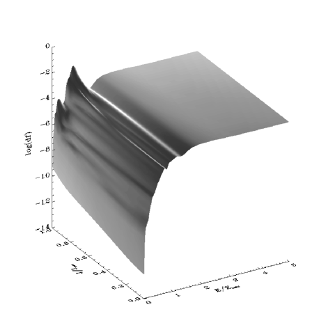
Figure 8: Even part of the distribution function obtained with a mass model of NGC 3115 including a central dark mass of ${M_{\rm BH}}=1.0\;10^{9}$ $\mbox{M}_{\sun}$: the logarithm of the distribution function is plotted as a function of the normalized energy $E/E_{max}$ and angular momentum $J/J_{max}$. $E_{max}$ corresponds to the central potential of the model when the central dark mass is excluded.

A number of models have thus been built, including different cusp slopes and a range of values for the mass to light ratio $M/L_{V}$ and for the central dark mass ${M_{\rm BH}}$. In Fig. 8, we present one example of such a distribution function obtained for $\rho\propto r^{-1.5}$ and ${M_{\rm BH}}=1.0\times 10^{9}$ $\mbox{M}_{\sun}$as a function of the normalized energy ($E_{max}$ corresponds to the central potential of the model excluding the central dark mass) and angular momentum ($J=J_{max}$ corresponds to circular orbits at a given energy). The double disc structure is clearly visible as two bumps near the line of maximum angular momentum, and the plateau at high energy corresponds to the cusp (for a cusp slope $\gamma=-1.5$ and a keplerian potential the distribution function is constant with energy, see Qian et al. 1995).

5.2 The inner 45 arcseconds

Figure 9: Observed kinematics (losanges) along the major-axis (two top panels) and the minor-axis (bottom panels) for the data of KR92 and the best fit model with ${M_{\rm BH}}=0.94\times 10^{9}$ $\mbox{M}_{\sun}$.

As shown in Sect. 4, an overall good fit to the data inside $40\arcsec$ requires a rather high mass to light ratio $M/L_{V}\sim 6.5$. For the best sets of data (namely vdM+94, CJ93, and KR92) which cover these radii, we built models with different central dark mass concentrations. In Fig. 9 we present the KR92 data set which extends further than $40\arcsec$ and overimposed the best fit model which includes a central dark mass of ${M_{\rm BH}}=0.94\times 10^{9}$ $\mbox{M}_{\sun}$and has a mass to light ratio $M/L_{V}=6.1$. The major-axis velocity and dispersion (best gaussian $V$ and $\sigma$) profiles are well fit by this model even in the inner part. The fit is also good along the minor-axis besides a significantly lower dispersion around $3\arcsec$ where the central dark mass starts to dominate the observed kinematics. The fit to the data of CJ93, which has a slightly higher spatial resolution, is also excellent.

Figure 10: Observed kinematics (open squares) along the major-axis for the data published in vdM+94, derived using the method described by Rix & White (1993). These data have been fit simultaneously on both sides of the centre (see vdM+94 for details). The best fit 2I model with ${M_{\rm BH}}=0.94\times 10^{9}$ $\mbox{M}_{\sun}$ is superimposed with (dotted line) and without (solid line) spectral filtering.

In Figure 10 we present the fit to the vdM+94 data set. In this case, the higher order Gauss-Hermite moments could also be included. We could not obtain a reasonable fit to the $h_{3}$ parameter for which the 2I model predicts values around -0.25 at $R\sim 25\arcsec$ while the observed one is $\sim-0.16$. It is possible to reduce (in absolute value) the predicted $h_{3}$ by changing the odd part of the distribution function, but at the expense of a significantly lower velocity $V$. Note that the predicted $h_{3}$ does not depend on the mass to light ratio (assuming it is constant with radius).

Uncertainties due to errors in the positioning of the slit or to spectral filtering (see Sect. 2.4) of the LOSVDs are far too small to fully account for this discrepancy. The effect of the latter is shown in Fig. 10 where the predicted LOSVDs have been slightly Fourier filtered before measuring the Gauss-Hermite moments: the fit is then significantly better for all $h_{3}$, $h_{4}$, $h_{5}$, $h_{6}$ profiles, without changing $V$ and $\sigma$ significantly. However, the filtering required to explain the data is large considering the signal to noise ($S/N\sim 20$ per 10 km.s^-1) and spectral resolution ($\sigma_{inst}\sim 23$ km.s^-1) quoted by vdM+94. We then performed some extensive simulations to derive the effect of the deconvolution method (Fourier fitting of the LOSVD) on $V$ and $h_{3}$: it is indeed significant for $R\sim 25\arcsec$, where it can reach $15$ $\mbox{km.s}^{-1}$and $\sim 0.04$ respectively. The data of vdM+94 are thus consistent with $h_{3}=-0.2$ at $R\sim 25\arcsec$, still too low in absolute value to be reconciled with our two-integral model. There are finally uncertainties associated with the data as illustrated in Fig. 11: the same 2I model is compared with the kinematics obtained by vdM+94 but this time derived using a one side Fourier-fitting technique (see vdM+94 for details). The fits to the higher order moments are good, although the predicted $V/\sigma$ is now too low.

Figure 11: Observed kinematics (open squares) along the major-axis for the data of vdM+94, derived from a Fourier fitting method. Here the data has been derived on each side of the centre independently (north-east side: open triangles; south-west side: open squares). The best fit 2I model with ${M_{\rm BH}}=0.94\times 10^{9}$ $\mbox{M}_{\sun}$ is superimposed (solid lines).

5.3 The central arcseconds

Figure 12: Central LOSVDs: observed FOS (thin solid line, shifted to zero velocity), directly predicted from model M1 (dotted line), and the same obtained via FCQ and using the characteristics of the FOS central spectrum (thick solid line).

The observed kinematics in the central arcseconds is very sensitive to the spatial resolution, particularly in the case of NGC 3115 for which both the photometry and kinematics exhibit large central gradients. But as we have shown in Sect. 2.4.1, the procedures used in the analysis of the data do also affect the final result. In the following paragraphs, we used the data provided by the FOS/HST and SIS spectrographs in parallel with the (lower resolution but) two-dimensional TIGER kinematics to constrain the free parameters of the dynamical models. We again examined a large range of different models, varying the central dark mass, the mass to light ratio, the central cusp slope as well as the odd part of the two-integral distribution function. For reasons of clarity, we only present here a few of these models which fit the data well.

Figure 13: Observed FOS kinematics along the major-axis (K+96, crosses), compared with the velocity and dispersion profiles predicted by models M1, M2 and M3 (thin solid, dotted and thick solid lines respectively) via FCQ and using the characteristics of the FOS data.

5.3.1 Best fit models

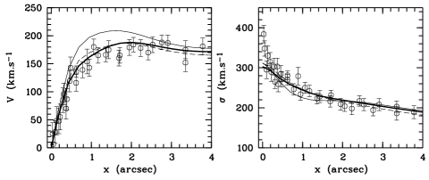
Figure 14: Observed SIS kinematics along the major-axis (K+96, circles), with the thin solid, dashed and thick solid lines corresponding to predictions of models M1, M2 and M3 respectively.

All our two integral models predict rather high $h_{4}$ values ($>0.08$) when ${M_{\rm BH}}$ is a few $10^{8}$ $\mbox{M}_{\sun}$. Our best fit model to the FOS data only has a cusp with $\rho\propto r^{-1.5}$ and a flattening of 0.7, a central mass ${M_{\rm BH}}=1.0\times 10^{9}$ $\mbox{M}_{\sun}$ and $M/L_{V}=6.5$ (model M1, see Fig. 13), although the cusp slope and flattening are not well constrained by the present data. In Fig. 13, we present the kinematical profiles obtained from the FOS spectra and model M1. The overall agreement is good, but our two integral model predicts a slightly higher central velocity dispersion with $\sigma(0)=480$ km.s.^-1. We should note however that the best gaussian fit to the LOSVD obtained by K+96, and presented in their Fig. 3 has $\sigma(0)\sim 489$ km.s^-1, significantly larger than the one derived via FQ, but consistent with our value. This point is emphasized in Fig. 12 where we now present the comparison between the FOS LOSVD obtained by K+96 and the one predicted by model M1. The agreement is excellent, considering that the wiggles present in the FOS central LOSVD are almost certainly not real (as are the negative points), but resulting from the presence of noise in the FOS spectrum as well as the template mismatching. It is striking to see the difference between the LOSVD directly predicted from model M1 and the one retrieved via FCQ using the same spectral filtering than for the FOS data: this forces us here to underestimate $h_{4}$ and correspondingly to overestimate the gaussian dispersion (see Sect. 2.4.1).

Model M1 includes a rapidly rotating nuclear disc with $a=5$ (see Section 5.1). This model predicts velocities which are clearly too high at the SIS resolution, as shown in Fig. 14. Kormendy et al. (1998) noticed the fact that, for SIS data of NGC 3377, FCQ seems to provide slightly higher velocities than FQ by about 10% (e.g. see their Fig. 15). If this is also the case for NGC 3115, it could reconcile our model M1 with the SIS data.

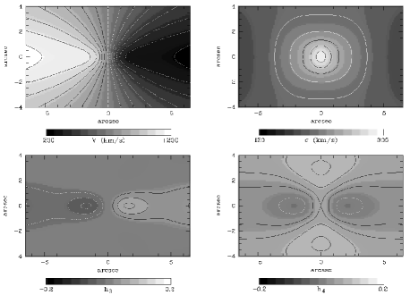
Figure 15: Predicted 2D kinematics for the TIGER setup from model M1. From top to bottom, left to right: $V$, $\sigma$, $h_{3}$ and $h_{4}$. Contours are the same than in Fig. 1.

We calculated other models where the parameter $a$ was significantly increased (up to $a=100$) for stars with high energy (close to the centre as we deal with positive energies): in this region the total distibution function tends towards the maximum streaming two-integral model. Fig. 13 and Fig. 14 present two other models, respectively M2 which corresponds to ${M_{\rm BH}}=1.24\;10^{9}$ $\mbox{M}_{\sun}$and $M/L_{V}=5.4$, and M3 which has ${M_{\rm BH}}=0.94\;10^{9}$ $\mbox{M}_{\sun}$and $M/L_{V}=6.1$. Although model M2 is a better fit to the FOS velocity and dispersion profiles, the higher black hole mass implies $h_{4}=0.134$, a value at the upper limit of the error bar mentioned by K+96. Model M3 is the best fit to the SIS data, and represents the best compromise to the HST data with a measured central $h_{4}=0.094$. These models also show that the detailed kinematical structure inside $0\aas@@fstack{\prime\prime}3$ remains ill constrained. Although stellar orbits may be biased towards near maximum angular momentum values in the central 10 pc, it is thus yet improper to discuss the internal kinematical structure of the point-like nucleus detected in the photometry (Sec. 3), all the more since its luminosity distribution is uncertain as well (see Fig. 4).

5.3.2 The TIGER data

We finally compare the three best fits (M1, M2 and M3) to the kinematics obtained with TIGER. Although the resolution of these data is significantly lower than the SIS data, it still represents a good constraint as it homogeneously covers a two-dimensional field on the sky. As seen in Fig. 1, the TIGER isovelocities are significantly flattened. This suggests again that the nuclear disc is rapidly rotating. The contrast between the disc and the central spheroid is however weaker than in the case of the Sombrero galaxy for which very asymmetric LOSVDs (and therefore high $h_{3}$ values) are observed at the centre (Wagner et al. 1989; Emsellem et al. 1996). All three models, M1, M2 and M3, fit reasonably well the TIGER kinematical maps, with M1 giving the smallest residuals. The kinematical maps corresponding to model M1 are presented in Fig. 15.

The results presented in the previous Sections, using two integral $f(E,J)$ models to fit the observed kinematics, can thus be summarized in a few points:

• There is a significant discrepancy between the observed and predicted $h_{3}$ values at a radius of about $25\arcsec$.

• The fit of the central FOS kinematics requires the nuclear disc to have a nearly maximum streaming distribution function inside $1\arcsec$.

• All the available kinematics in the central arcseconds can be rather well fit by a two-integral model with constant mass to light ratio. The best constrained parameters are the central dark mass and the mass to light ratio: considering the error bars in the different data sets, our best estimations are ${M_{\rm BH}}=0.94^{+0.35}_{-0.2}\;10^{9}$ $\mbox{M}_{\sun}$and $M/L_{V}=6.1^{+0.5}_{-0.7}$. These values can be refined using the higher order Gauss Hermite moments in the central arcsecond. However the observed kinematics are very sensitive to the details of the instrumental setup and the analysis procedures.

We could in principle reconcile our 2I model with the observed kinematics along the major-axis. The input mass model has been indeed derived from a $V$ band image which may not reflect the true mass distribution. We have for example assumed that the bulge and disc components have the same mass to light ratio. This is certainly not true since they do not share the same colour profiles (Fisher et al. 1996). A difference of 0.1 magnitude in $B-R_{c}$ as typically observed between the bulge and the disc regions in NGC 3115 (Fisher et al. 1996) corresponds to a maximum change of about 5% in $M/L_{V}$ (Worthey et al. 1994), too small an effect to account for the discrepancy in $h_{3}$. In the following, we wish to examine another explanation: the distribution function depends on a third integral of motion. A two integral distribution function $f(E,J)$ imposes that $\sigma_{R}=\sigma_{z}$ everywhere. This may not be the case for the S0 galaxy NGC 3115, as for our own Galaxy. This is also supported by derivations kindly made by Roeland van der Marel, using the formalism described in de Bruijne et al. (1996) which allows a rather general geometry of the velocity ellipsoid. Although these models cannot mimic the complex morphology of NGC 3115, they clearly suggest that, for very flattened components, low $h_{3}$ values of the order of $-0.2$ could be obtained by relaxing the constraint of a two-integral distribution function.

6 A three integral distribution function

In this Section, we will construct a three-integral model using a quadratic programming technique. With the three integral modeling, we wish to approach two questions

1. Is it possible to fit the data without a central dark mass, with a distribution function that has the appropriate three integral structure? In this context, we recall the well-known case of M87, where Binney & Mamon (1982) succeeded in fitting the (then available) data with a distribution function that was very anisotropic.

2. What is the phase-space structure of the best global 3I model?

This is an opportunity to present the use of the Quadratic Programming technique on a complex object, using a complete set of two-dimensional kinematical data. It should be clear from the outset, however, that we chose to produce analytical distribution functions. These implies that our third integral must be approximate. In that sense, the three integral models we present here must be seen as belonging to the class of models with approximate third integrals.

6.1 The method

The essence of the method relies on the fact that most, if not all, observable kinematic quantities can be expressed as linear functionals of the distribution function, if the potential is given. This means that if we approximate the distribution function $f$ as a sum of some conveniently chosen basis functions $f_{i}$:

$$f=\sum_{i}c_{i}f_{i}(I_{1},I_{2},I_{3}),$$ (2)

then the same relation holds between the (e.g.) projected mass density $\rho_{p}$ and the projected mass density of the components $\rho_{p,i}$

$$\rho_{p}=\sum_{i}c_{i}\rho_{p,i},$$ (3)

or a similar relation for the projected pressures:

$$\rho_{p}(\sigma_{p}^{2}+\langle v_{p}\rangle^{2})=\sum_{i}c_{i}[\rho_{p}(\sigma_{p}^{2}+\langle v_{p}\rangle^{2})]_{i}.$$ (4)

If we stick to the mass density $\rho$ for simplicity, we can construct a $\chi^{2}$ variable with the observed values $\rho_{l}$ as follows:

$$\chi^{2}=\sum_{l}w_{l}\left(\rho_{l}-\sum_{i}c_{i}\rho_{i,l}\right)^{2},$$ (5)

with $\rho_{i,l}$ the value of the mass density at the $l-$th point for component $i$, and the $w_{l}$ associated weights. Clearly this $\chi^{2}$ is quadratic in the coefficients $c_{i}$. Inclusion of other observables is trivial.

The minimisation of such a $\chi^{2}$ will produce a set of coefficients, which will yield a distribution function (2) that will not necessarily be positive everywhere. Therefore, one must include constraints

$$\sum_{i}c_{i}F_{i}[(I_{1},I_{2},I_{3})_{m}]\geq 0,\qquad m=1,\ldots,M,$$ (6)

expressing the positivity of the distribution function on a grid in phase space with points $(I_{1},I_{2},I_{3})_{m}$. This formulates a problem of quadratic programming, which is a well-known problem for which efficient algorithms exist.

In the present case, we use the luminosity model as presented in section 3. As discussed in Sect. 4, a constant M/L model will not work at large radii. This is indicated by the rotation curve, which is almost flat up to $200^{\prime\prime}$ (Capaccioli et al. 1993). We therefore construct a model for the dark mass that preserves the form of the luminous mass (say, for simplicity of the argument, ellipses with fixed axis ratios and semi-major axes $a$) and that has the radial dependence

$$\rho_{\rm tot}(a)=\rho_{\rm lum}(a)(1+Ca^{p}).$$ (7)

We used $p=1.5$, and the coefficient $C$ is such that

$${\rho_{\rm tot}(a)\over\rho_{\rm lum}(a)}=30,\qquad a=30{\rm kpc}.$$ (8)

This prescription produces a flat rotation curve. In practice, we adopt the same shape for the dark matter as for the luminous mass density, by specifying the relation (7) for all the radial functions in the harmonic expansion of $\rho_{\rm lum}$. In Table 4, we present the dependence of the mass to light ratio of the three-integral model on the radius in the equatorial plane. For the sake of comparison, we will also present in Sect. 6.2 a model where the mass to light ratio was forced to stay constant (besides the central dark mass).

Table 4: Mass to light ratio of the three-integral model versus the radius in arcsec or kpc. The contribution of the luminous mass is given in the right column

$R$	$R$	$M/L_{V}$	$M_{lum}$
(kpc)	($\arcsec$)		(%)
0.1	21	5.8	100
1.5	30	6.1	90
2.9	60	9.9	79
4.4	90	13.9	68
5.8	120	19.9	59
7.3	150	26.0	52
8.7	180	32.5	46
10.2	210	39.5	41
11.6	240	46.9	38
13.1	270	54.4	35
14.5	300	63.1	33

The calculation of the potential is straightforward, when the harmonic expansion of the total mass density is given. In practice, we interpolate the potential on a grid. Since it is our goal to explore what three integral dynamical model contributes to the modeling of NGC 3115, we need an expression for the third integral $I_{3}$. This is done by fitting the potential with a Stäckel potential, and adopting the third integral from the Stäckel case as our approximation of the third integral. Thus, our models belong to the class of 3I models that use an approximation for the third integral. The procedure is outlined in more detail in Dejonghe et al. (1996).

Finally, we include a central singularity. It is a softened $1/r$ singularity (hence a Plummer sphere), with a softening length of the order of 50000 AU ($\sim 0.25$ pc or $\sim 5$ mas, about forty times smaller than the FOS aperture). In the transition region where the gravitational force of the black hole is of comparable strength as the gravitational force of the core of the galaxy, there is no third integral and the Stäckel approximation of the potential is probably invalid. However, as argued in Sect. 4, we adopt as our working hypothesis that the spheroidal central component is two-integral. Hence, it will suffice if we produce three-integral models that do no penetrate too deep into the centre, where the model thus remains two-integral. It is however important to note that since orbits are non-local, the three-integral nature of our models significantly extends the probed space of solutions.

The data we use to build the $\chi^{2}$ are photometric and kinematical. As for the photometry, we produce a series of data points taken from a (logarithmically spaced) grid of the deprojected luminous mass density as obtained in Sect. 3. The kinematical data for this modeling part are twofold.

• Outside $50\arcsec$ along the major-axis and $8\arcsec$ along the minor-axis, the effect of pixel integration and seeing convolution is negligible, and we assumed that the gaussian velocity and dispersion are good approximations for the two first true moments. We thus selected a set of points from the above mentioned sources. It is impractical (yet) to include all data points, while some are, mildly inconsistent.

• The rest of the galaxy (mainly the central part and the major-axis inside $50\arcsec$) was sampled using the estimations of the true moments given by the TIGER data presented in Sect. 2.2.1 and the published kinematics of vdM+94. This of course required to include the instrumental setup in the $\chi^{2}$.

As for the components, we use two families. The first one is an extention of Fricke components, and has distribution functions of the form

$$F_{pmnE_{0}J_{0}}^{\pm}=(E-E_{0})^{p}(J-J_{0})^{2m}I_{3}^{n}$$ (9)

wherever $\pm J\geq J_{0}$ and $E>E_{0}$. They are zero elsewhere. The exponent $m$ and $n$ are an integer, but $p$ can be real. In general the parameter $p$ controls the central concentration of the component, the parameter $q$ controls the amount of angular momentum, while $n$ is indicative of the dependence on the third integral. The cut-off binding energy $E_{0}$ is needed to limit the extent of the components, for further enhanced flexibility. Also, since the potential is almost singular at the centre, large values of $p$ (thus components that are concentrated) produce impossibly high mass densities at the centre. Hence, we rather control the central concentration with the parameter $E_{0}$, and adopt low or even fractional values for $p$. Finally, the cut-off angular momentum $J_{0}$ prohibits the orbits to penetrate too deep into the potential well, where the third integral may not exist.

The second family is designed to produce very thin 2I discs in the equatorial plane of the galaxy (Batsleer & Dejonghe 1995), and has members of the form

$$F_{pqs}^{\pm}=(S_{z_{0}}(J))^{p}J^{2q}(E-S_{z_{0}}(J))^{s}$$ (10)

wherever $\pm J\geq 0,E>S_{z_{0}}(J)$. They are zero elsewhere. The parameters $p$, $q$ and $s$ can be real. The quantity $S_{z_{0}}(J)$ is the maximum binding energy that a star with angular momentum $J$ can have if its distance from the equatorial plane remains below $z_{0}$. If $z_{0}=0$, $S_{0}(J)$ is the binding energy of a circular orbit with $J$. The parameters $p$ and $q$ have the same meaning as in the first family, while $s$ controls the concentration of the component towards the equatorial plane.

6.2 Results

Figure 16: Data points from B+94 (triangles) and vdM+96 (crosses), and the best fit (3I models) with a $6.5\times 10^{8}$ $\mbox{M}_{\sun}$black hole (solid line) and best fit for a model without black hole (dotted line). The models have been convolved to correspond to B+94 data.

Figure 17: A comparison of the luminous mass density, as obtained by the MGE technique (solid lines), and the 3I fit (dotted or dashed lines). The upper left panel shows the log of the luminous mass density along the major axis, the upper right panel dito along the minor axis

In Fig. 16 we compare two models on the major axis, within the central $8^{\prime\prime}$. The solid line corresponds to a model with a $6.5\times 10^{8}$ $\mbox{M}_{\sun}$black hole, the dashed line has no black hole. Clearly, even in the three-integral case, the latter model fails dismally, especially in the inner $2\arcsec$. This is to be expected of course: the large dispersion in the centre exceeds the escape velocity if no black hole is present. Any reshuffling of orbits in order to obtain a favourable viewing position is insufficient in the absence of a black hole, because there is simply not enough kinetic energy present. Although new components not included in our library may help, this is a strong suggestion that even three-integral models without a black hole cannot fit the data.

In fact, if we compactify integral space by considering the representation in ($E$, $J\sqrt{E}$, $I_{3}E$) then powers, such as Fricke components, form a complete set, if one allows negative coefficients. In practice, of course, one is limited by finite computing resources. But at least, all orbits are present, with relative weights that vary continuously, and thus not necessarily with arbitrarily flexible relative weights. However, this practical incompleteness is not fundamentally different from the one present in, say, the Schwarzschild method. In the latter case, phase space cannot be covered completely, also for practical reasons, but the orbits considered can have arbitrarily flexible relative weights, at least without the (necessary) smoothing. So both methods are incomplete in practice, be it to varying degree, but the incompleteness certainly will manifest itself differently.

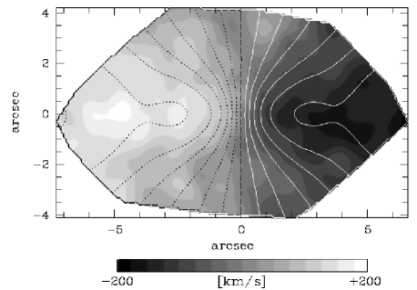
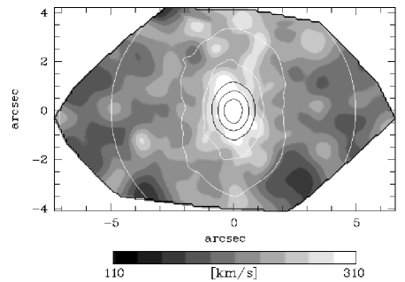
Figure 18: The TIGER maps of the first true velocity moments $\tilde{V}$ (upper panel) and $\tilde{\sigma}$ (lower panel), compared to the three-integral model with ${M_{\rm BH}}=6.5\times 10^{8}$ $\mbox{M}_{\sun}$(contours: step of 20 $\mbox{km.s}^{-1}$for $\tilde{V}$ and 25 $\mbox{km.s}^{-1}$for $\tilde{\sigma}$).

Regarding our second question, we first compare in Fig. 17 the luminous mass density as obtained with the MGE technique (see Section 3) with the best 3I model that has a black hole of $6.5\times 10^{8}$ $\mbox{M}_{\sun}$(see also Fig. 4). The fit is quite reasonable, certainly considering the dynamic range that is to be covered (see upper panels).

In Fig. 18, 19 and 20 we next compare the input kinematical data with our best model that has a black hole of $6.5\times 10^{8}$ $\mbox{M}_{\sun}$and includes a dark halo. The fit is good, except perhaps at the centre along the cut $y=20\arcsec$ and the one $x=40\arcsec$ (Fig. 20). In fact, the data (Illingworth & Schechter 1982) presented in this plot are mildly inconsistent with other published data along the minor or major axis (e.g. vdM+94, see Fig. 19). The model with a constant mass to light ratio ($M/L_{V}=10$, dotted lines in Fig. 19 and 20) does however show significant discrepancies along the major-axis and the cut $y=20\arcsec$, with an overestimate of the velocity in the inner $50\arcsec$. This shows, as already stated, that the mass to light ratio must significantly increase outwards, by nearly a factor of 2 between the inner parts ($R<50\arcsec$, $M/L\sim 6$) and the last measured point ($R\sim 200\arcsec$, $M/L_{V}\sim 10$). We therefore confirm what was suggested by C+93 via simple dynamical arguments, but here using general three-integral dynamical models. Although a stellar mixture with a global $M/L_{V}\sim 10$ is not excluded, it would have to be reconciled with the nearly constant (but decreasing) colours in the outer parts of NGC 3115 (for $R>120\arcsec$, Strom et al. 1977) and the metal poor populations observed in the halo by Elson (1997). The major-axis velocity and dispersion profiles are also more consistent with flat curves than with falling ones (see Fig. 19 and Fig. 20): this suggests that the $M/L_{V}$ is still significantly increasing outwards for $R>150\arcsec$. In the view of these two points, we favour the hypothesis of the presence of a dark halo to explain the observed kinematics of NGC 3115 at large radii.

Figure 19: A comparison of the kinematics along the major-axis and the best fits with a $6.5\times 10^{8}$ $\mbox{M}_{\sun}$black hole: including a dark halo (solid lines) or with a constant $M/L_{V}=10$ (dotted lines). Inside 40 arcseconds we compare the model to the data of vdM+94, and outside this radius to the data of Capaccioli et al. (1993). The models have been convolved accordingly.

Figure 20: A comparison of the data points of Illingworth & Schechter (1982) and the best fits with a $6.5\times 10^{8}$ $\mbox{M}_{\sun}$black hole: with a dark halo (see text, solid lines) and with a constant $M/L_{V}=10$ (dotted lines). For each cut, we present the velocity (lower panel) and dispersion (upper panel). Note that the discrepancies between the model with the dark halo (solid lines) and the data are mostly due to inconsistencies in the data itself.

For efficiency reasons, we included values for the hermite coefficients at only 2 radii . At $7^{\prime\prime}$, the model convolved at the resolution of vdM+94 data has $h_{3}=-0.0025$, close to the observed $h_{3}=-0.05$, and in fact consistent with other published $h_{3}$ at this radius (Bender et al. 1994, F96). At $26^{\prime\prime}$ we obtain $h_{3}=-0.15$, a much better fit than the 2I result, now perfectly consistent with the observed $h_{3}=-0.16$. In fact all observed higher order moments are now reasonably fit by the three-integral model.

Finally, we present in Fig. 21 and Fig. 22 the mean rotation and velocity dispersions of the model in a meridian. The inner disc is tangentially anisotropic with $\sigma_{\phi}/\sigma_{r}$ reaching a value of $\sim 0.6$ in the inner $2\arcsec$. This confirms the finding obtained via the two-integral model in Sect. 5 that the inner disc seems to be close to maximum rotation. Between $3\arcsec$ and $15\arcsec$ in the equatorial plane, the model is nearly isotropic. The inner spheroid ($R<60\arcsec$) is close to two-integral and has a nearly constant $\sigma_{\phi}/\sigma_{r}\sim 0.65$. Going outwards, the distribution function becomes significantly three-integral and more radially anisotropic. Already at a radius of $30\arcsec$ in the equatorial plane ($R\sim 1.5$ kpc) $\sigma_{z}/\sigma_{r}\sim 1.1$ and $\sigma_{\phi}/\sigma_{r}\sim 0.8$. The ratio $\sigma_{\phi}/\sigma_{r}$ reaches a local maximum of $0.92$, at a radius of $\sim 100\arcsec$, where the outer disc contribution disappears and the dark matter becomes dominant.

Figure 21: Some moments of the best fit 3I distribution function in a meridian. Upper panel: $\langle v\rangle$ and lower panel: $\sigma_{\phi}$.

Figure 22: Some moments of the best fit 3I distribution function in a meridian. Lower panel: $\sigma_{r}$ and upper panel: $\sigma_{z}/\sigma_{r}$.

7 Conclusions

We have presented a detailed analysis of the kinematics of NGC 3115 using different modeling techniques. As far as possible, we have made use of the photometric and kinematical data available to us, in order to build dynamical models following realistic light and mass distributions. For the first time, we have included two-dimensional spectroscopic data in order to constrain the models in the central few hundred parcsecs.

Jeans equations were used to define reasonable ranges for the mass to light ratio and the central dark mass in the frame of a two integral dynamical model. Fitting the first two velocity moments in the central $40\arcsec$ gives ${M_{\rm BH}}=6.5\pm 3.5\times 10^{8}$ $\mbox{M}_{\sun}$ and $M/L_{V}=6.5\pm 0.7$. These estimations were then tested by retrieving the corresponding distribution functions via the Hunter & Qian method (Sect. 5). We would like to emphasize the fact that a simple two-integral model with a constant mass to light ratio can fit the velocity and dispersion profiles of NGC 3115 inside $\sim 45\arcsec$ surprisingly well (see Sect. 5).

However, no two-integral model could fit the value of $V$ and $h_{3}$ simultaneously as observed by vdM+94 around $25\arcsec$ along the major-axis, where the outer disc significantly contributes to the surface brightness. Models built using the quadratic programming technique confirmed that three integral components solve this problem (Sect. 6). The dynamical structure of the outer part of NGC 3115 is therefore very probably three-integral.

In Sect. 5, we showed that there are no two integral axisymmetric models which can fit the kinematics of NGC 3115 in the central region, without the addition of a central dark mass of about $10^{9}$ $\mbox{M}_{\sun}$. The best fit, which makes use of FOS/HST (Kormendy et al. 1996) and Gauss-Hermite moments, was obtained for ${M_{\rm BH}}=0.94\times 10^{9}$ $\mbox{M}_{\sun}$and $M/L_{V}=6.1$. This estimation of the central dark mass is at the upper limit of the range derived from simple Jeans models. This shows the need of high spatial resolution kinematics including the higher order moments in order to more accurately constrain the mass distribution.

The quadratic programming technique confirmed the need of a central dark mass as even the three-integral models without a black hole failed to fit the central rise in the velocity dispersion. In principle, one could object that, since a library of 3I distribution functions is always limited, no matter what method is considered for the modeling, this is no definite proof that a roughly constant $M/L$ model cannot fit the observables. However such a model would have to populate a lot of stars on radial orbits in the very centre. This would produce a galaxy core that is extremely prone to radial orbit instabilities, which, given the dynamical time of the order of $8\times 10^{6}$ years at a radius of $10\arcsec$ ($\sim 500$ pc), would have relaxed into a more stable configuration a long time ago, or would have produced a bar, evidence of which is not (yet) present.

Previous estimations of the central dark mass in NGC 3115 are surprisingly different from one paper to the other. Kormendy & Richstone (1992) derived a value of ${M_{\rm BH}}$ from 1 to $2\times 10^{9}$ $\mbox{M}_{\sun}$using spherical models corrected for flattening. Then Kormendy et al. (1996), using the same formalism, confirmed the upper limit of $\sim 2\times 10^{9}$ $\mbox{M}_{\sun}$by including the SIS and HST/FOS data. Both papers used a mass to light ratio of $M/L_{V}\sim 4$. Finally, Magorrian et al. (1998) found a best fit value of ${M_{\rm BH}}\sim 4.8\times 10^{8}$ $\mbox{M}_{\sun}$with a $M/L_{V}\sim 6.75$ (both values scaled for $D=10$ Mpc), noting that their value for ${M_{\rm BH}}$ was probably an underestimate. This is consistent with the picture drawn in the present work since we find that a value of ${M_{\rm BH}}$ as low as $6.5\times 10^{8}$ $\mbox{M}_{\sun}$(with a corresponding $M/L_{V}=6.8$) is compatible with the existing data. However, our best fit model has ${M_{\rm BH}}=0.94\times 10^{9}$ $\mbox{M}_{\sun}$, and values as high as ${M_{\rm BH}}=2\times 10^{9}$ $\mbox{M}_{\sun}$are excluded at more than the 3$\sigma$ level. Our models, because they more precisely follow the observed light distribution and include the derivation of the full distribution function, are improved estimations of the central dark mass and mass to light ratio.

We finally showed that the mass to light ratio should increase by a factor of two between the inner parts ($R<50\arcsec$) and the outer parts ($R>100\arcsec$) of NGC 3115. We produced a model which fits the flat rotation and dispersion profiles along the major-axis and thus gave the first evaluation of the amount of dark matter required to explain the observed kinematics at large radii: in our model the dark matter represents about 50% of the total mass inside $150\arcsec$ and nearly 70% inside $300\arcsec$. These values are obviously still uncertain as we did not fully examine alternative spatial distributions or radial profiles.

Appendix A Convolution and pixel binning using a kernel

It is possible to combine pixel integration and PSF smearing in only two integrals (as otherwise would be four: two for the seeing and two for the pixel integration). This is described in the following in the case of circular or rectangular pixels (see also Qian et al. 1995)

A.1 Circular pixel

For a circular pixel (TIGER like lenses) of radius $d$, the observable $S_{o}$ at a position $(x^{\prime},y^{\prime})$ after convolution with a single gaussian of dispersion $\sigma$ and integration on the pixel is:

$$S_{o}(x^{\prime},y^{\prime}) = \frac{1}{\pi d^{2}}\times\int_{0}^{\infty}rdr\int_{0}^{2\pi}d\theta K(r)$$ (11)

$$S\left[x^{\prime}+r\cos{\left(\theta+\theta_{0}\right)},y^{\prime}+r\sin{\left(\theta+\theta_{0}\right)}\right]$$

where:

$$K(r)=\int_{0}^{d/\sigma}s\;ds\;I_{0}\left(\frac{sr}{\sigma}\right)e^{-\frac{sr}{\sigma}}e^{-\frac{1}{2}(s-r/\sigma)^{2}}$$ (12)

Note that if the integrals are derived with fixed quadratures, the Kernel has only to be calculated once, and only depends on the radius $r$.

A.2 Rectangular pixel

For a rectangular pixel of dimension $2l\times 2w$. The observable $S_{o}$ at a position $(x^{\prime},y^{\prime})$ after convolution with a single gaussian of dispersion $\sigma$ and integration on the pixel is:

$$S_{o}(x^{\prime},y^{\prime}) = \frac{1}{4lw}\times\int_{0}^{\infty}rdr\int_{0}^{2\pi}d\theta K(r,\theta)$$ (13)

$$S\left[x^{\prime}+r\cos{\left(\theta+\theta_{0}\right)},y^{\prime}+r\sin{\left(\theta+\theta_{0}\right)}\right]$$

where:

$$K(r,\theta) = \frac{1}{4}\times\left[{\rm erf}\left(\frac{l+r\cos{\theta}}{\sqrt{2}\sigma}\right)-{\rm erf}\left(\frac{-l+r\cos{\theta}}{\sqrt{2}\sigma}\right)\right]$$ (14)

$$\times\left[{\rm erf}\left(\frac{w+r\sin{\theta}}{\sqrt{2}\sigma}\right)-{\rm erf}\left(\frac{-w+r\sin{\theta}}{\sqrt{2}\sigma}\right)\right]$$

and note again that if the integrals are derived with fixed quadratures, the Kernel can be calculated only once on a fixed grid.

Appendix B Cusps in MGE photometric models

As we wish to build photometric models which can reproduce central power laws, it has been necessary to extend the MGE formalism (Emsellem et al. 1996) to include such cusp components. The adopted form for the central component is then:

$$\nu(m_{c}^{2})=I_{c}\cdot\left(\frac{m_{c}^{2}}{2\cdot\sigma_{c}^{2}}\right)^{-\gamma/2}\times\exp{\left\{-\frac{m_{c}^{2}}{2\cdot\sigma_{c}^{2}}\right\}}$$ (15)

where $m_{c}^{2}=R^{2}+Z^{2}/q_{c}^{2}$. This is the natural generalized form of the 3D gaussian function.

The integrated luminosity of this component is $I_{c}\cdot 2\pi\left(\sqrt{2}\sigma_{c}\right)^{3}q_{c}\Gamma\left(1.5-\gamma/2\right)$, and the gravitational potential contribution simply:

$$\Phi(R,Z) = 4\pi Gq_{c}\sigma_{c}^{2}P_{c}\times$$ (17)

$$\int_{0}^{1}\frac{\Gamma\left(1-\gamma/2,\frac{T^{2}}{2\cdot\sigma_{c}^{2}}\left(R^{2}+Z^{2}/\left(1-e^{2}_{c}T^{2}\right)\right)\right)}{\left(1-e^{2}_{c}T^{2}\right)^{1/2}}\mbox{d}T$$

with $e^{2}_{c}=1-q^{2}_{c}$ and $P_{c}={\cal M/L}\times I_{c}$.

References

- [1] Bacon R. et al., 1995, A&AS, 113, 347
- [2] Bacon R., Emsellem E., Monnet G., Nieto J.L., 1994, A&A, 281, 691
- [3] Batsleer P., Dejonghe H., 1995, A&A, 294, 693
- [4] Bender R., 1990, A&A, 229, 441
- [5] Bender R., Saglia R. P., Gerhard O., 1994, MNRAS, 269, 785
- [6] Binney J., Mamon G.A., 1982, MNRAS, 200, 361
- [7] Byun Y. I., Freeman K.C., 1995, ApJ, 448, 563
- [8] Capaccioli M., Cappelaro E., Held E. V., Vietri M., 1993, A&A, 274, 69 (C+93)
- [9] Capaccioli M., Held E. V., Nieto J.-L., 1987, AJ, 94, 1519
- [10] Capaccioli M., Vietri M., Held E. V., 1988, MNRAS, 234, 335
- [11] Cretton N., van den Bosch F., 1998, submitted to ApJ
- [12] Dejonghe H., 1986, Phys. Rep., 133, 217
- [13] Dejonghe H., 1987, ApJ, 320, 477
- [14] Dejonghe H., 1989, ApJ, 343, 113
- [15] Dejonghe H., De Bruyne, V., Vauterin, P., 1996, A&A, 306, 363.
- [16] de Vaucouleurs A., Longo G., 1988, Univ. of Texas, Austin
- [17] Elson R. A. W., 1997, MNRAS, 284, 771
- [18] Emsellem E., 1995, A&A, 303, 673
- [19] Emsellem E., Monnet G., Bacon, R. 1994, A&A, 285, 723
- [20] Emsellem E., Bacon R., Monnet G. Poulain P., 1996, A&A, 312, 777
- [21] Fisher D., 1997, AJ, 113, 950 (F97)
- [22] Fisher D., Franx M., Illingworth G., 1996, ApJ, 459, 110
- [23] Hunter C., Qian E., 1993, MNRAS, 202, 401
- [24] Illingworth G., Schechter P. L., 1982, ApJ, 256, 481
- [25] Jarvis B. J., Freeman K. C., 1985, ApJ, 295, 314
- [26] Kormendy J., Richstone D., 1992, ApJ, 393, 559 (KR92)
- [27] Kormendy J., Bender R., Evans A., Richstone D., 1998, AJ, 115, 1823
- [28] Kormendy J., Bender R., Richstone D., Ajhar E. A., Dressler A., Faber S. M., Gebhardt K., Grillmair C., Lauer T. L., Tremaine S., 1996, ApJL, 459, 57 (K+96)
- [29] Magorrian J., Tremaine, S., Richstone D., Bender R., Bower G., Dressler A., Faber S. M., Gebhardt K., Green, R., Grillmair C., Kormendy J., Lauer T., 1998, AJ, 115, 2285
- [30] Monnet G., Bacon R., Emsellem E., 1992, A&A, 253, 366
- [31] Poulain P., 1986, A&AS, 64, 225
- [32] Poulain P., 1988, A&AS, 72, 215
- [33] Qian E. E., de Zeeuw P. T., van der Marel R. P., Hunter C., MNRAS, 1995, 274, 602
- [34] Seifert W., Scorza C., 1996, A&A, 310, 75
- [35] Silva D. R., Boroson T. A., Thompson I. B., Jedrzejewski R. I., 1989, AJ, 98, 131
- [36] Scorza C., Bender R., 1995, A&A, 293, 20
- [37] Strom K. M., Strom S. E., Jensen E. B., Moller J., Thompson L. A., Thuan T. X., 1977, ApJ, 212, 335
- [38] van den Bosch F., de Zeeuw P. T., 1996, MNRAS, 283, 381
- [39] van der Marel R. P., 1994, ApJL, 432, 91
- [40] van der Marel R. P., Cretton N., de Zeeuw P. T., Rix H.-W., 1998, ApJ, 493, 613
- [41] van der Marel R. P., de Zeeuw P. T., Rix H.-W., 1997, ApJ, 488, 119
- [42] van der Marel R. P., Rix H.-W., Carter D., Franx M., White S. D. M., de Zeeuw T., 1994, MNRAS, 268, 521 (vdM+94)
- [43] Wagner S. J., Dettmar R.-J., Bender R., 1989, A&A, 215, 243
- [44] Worthey G., 1994, ApJS, 95, 107