Vela X-1 as seen by RXTE

Abstract

We present results from four observations of the accreting X-ray pulsar Vela X-1 with the Rossi X-ray Timing Explorer (RXTE) in 1996 February.

The light curves show strong pulse to pulse variations, while the average pulse profiles are quite stable, similar to previous results. Below 5 keV the pulse profiles display a complex, 5-peaked structure with a transition to a simple, double peak above $\sim$15 keV.

We analyze phase-averaged, phase-resolved, and on-pulse minus off-pulse spectra. The best spectral fits were obtained using continuum models with a smooth high-energy turnover. In contrast, the commonly used power law with exponential cutoff introduced artificial features in the fit residuals. Using a power law with a Fermi-Dirac cutoff modified by photoelectric absorption and an iron line, the best fit spectra are still unacceptable. We interpret large deviations around $\sim$25 and $\sim$55 keV as fundamental and second harmonic cyclotron absorption lines. If this result holds true, the ratio of the line energies seems to be larger than 2. Phase resolved spectra show that the cyclotron lines are strongest on the main pulse while they are barely visible outside the pulses.

1 Introduction

Vela X-1 (4U 0900$-$40) is an eclipsing high mass X-ray binary consisting of the 23 $M_{\sun}$ B0.5Ib supergiant HD 77581 and a neutron star with an orbital period of 8.964 d (van Kerkwijk et al. (1995)), corresponding to an orbital radius of about $1.7\,{\rm R_{*}}$ (Fig. 1). The system is at a distance of 2.0 kpc (Sadakane et al. (1985)). Due to the closeness of the neutron star and its companion, the neutron star ($M$ $\sim$1.4 $M_{\sun}$, Stickland et al. (1997)) is deeply embedded in the strong stellar wind of HD 77581 ($\dot{M}\sim 4\,10^{-6}\,M_{\sun}/{\rm yr}$, Nagase et al. (1986)). Thus, the system is a prime candidate for the study of X-ray production via wind accretion. The X-ray luminosity is typically $\sim 4\,10^{36}\,{\rm erg/s}$, but can also suddenly change to less than 10% of its normal value (Inoue et al. (1984)). The reason for this variability is still unknown. It might be caused by changes in the accretion rate due to variations in the stellar wind or the formation of an accretion disk (Inoue et al. (1984)). For an in-depth discussion of the system parameters, see kerkwijk95a.

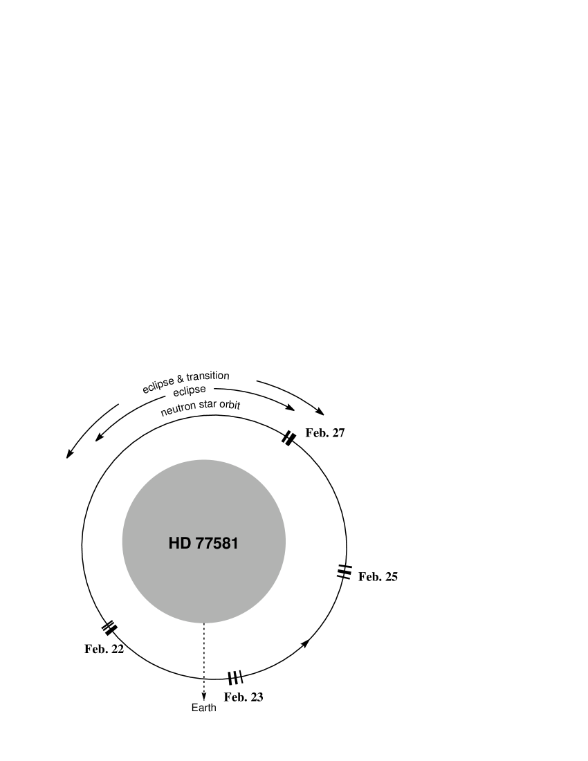
Figure 1: Sketch of the Vela X-1 system (center of system). The dashes mark the approximate orbital positions when the observations were made. The movement and the Roche-deformation of HD 77581 have been neglected.

Vela X-1 is a slow X-ray pulsar with a period of about 283 seconds (Rappaport & McClintock (1975)). Despite significant pulse-to-pulse variations, the pulse profile averaged over many pulses is quite stable (Staubert et al. (1980)). The profile changes from a complex five-peaked structure at energies below $\sim$5 keV to a simple double peaked structure at energies above $\sim$15 keV (Raubenheimer (1990)).

The X-ray spectrum of Vela X-1 is usually described by a power law with an exponential cutoff at high energies and an iron K$\alpha$ line at 6.4 keV (Nagase et al. (1986); White et al. (1983); Ohashi et al. (1984)). Below $\sim$3 keV, a soft excess is observed (Lewis et al. (1992); Pan et al. (1994)). The spectrum is further modified by photoelectric absorption due to a gas stream trailing the neutron star and due to circumstellar matter (Kaper et al. (1994)). This results in significantly increased absorption at orbital phases $\ga$0.5. In addition, erratic increases of $n_{\rm H}$ by a factor of 10 are seen at all orbital phases (Haberl & White (1990)). At energies above 20 keV, evidence for cyclotron absorption features at $\sim$27 keV and $\sim$54 keV has been reported from the High Energy X-Ray Experiment (HEXE) on Mir (Kendziorra et al. (1992)), from Ginga (Mihara (1995)), and from BeppoSAX observations (Orlandini et al. (1998)), but to date no statistically compelling result on both lines has been obtained.

In this paper we present the results of the analyses of four observations of Vela X-1 with RXTE. The observations and data reduction are described in Sect. 2. In Sect. 3 we discuss the light curves and pulse profiles. Section 4 is devoted to the spectral analysis, including spectral models, phase averaged spectra, phase resolved spectra, and a comparison with other instruments. Finally, we discuss the results in Sect. 5.

2 Observations and Data Analysis

We observed Vela X-1 with RXTE four times, covering nearly a complete binary orbit from phase 0.3 to 0.9. Each observation was between 5 ksec and 6 ksec long (see Table 1 and Fig. 1). The observations were carried out between 1996 February 22 and 1996 February 27. The exact time and duration of each observation are given in Table 1. In our analysis we used data from both RXTE pointing instruments, the Proportional Counter Array (PCA) and the High Energy X-ray Timing Experiment (HEXTE). To avoid scattered photons from the Earth, we used only data where Vela X-1 was more than $10^{\circ}$ above the horizon. To extract spectra and light curves, we used the standard RXTE analysis software FTOOLS 4.0 and software provided by the HEXTE instrument team at UCSD.

Table 1: Details of these observations of Vela X-1 with RXTE. The on source time corresponds only to the PCA.

No.	date	JD (center of	orbital	on source
		observation)	phase	time
1	1996 February 22	2450135.66	0.311–0.324	6048 s
2	1996 February 23	2450137.30	0.492–0.509	5696 s
3	1996 February 25	2450139.17	0.701–0.717	5536 s
4	1996 February 27	2450140.79	0.884–0.895	5820 s

The PCA consists of five co-aligned Xenon proportional counter units with a total effective area of about 6500 ${\rm cm}^{2}$ and sensitive in the energy range from 2 keV to $\sim$60 keV (Jahoda et al. (1996)). Light curves with 250 ms resolution and energy spectra in 128 pulse height channels were collected. For spectral fitting, we used version 2.2.1 of the PCA response matrices (Jahoda 1997, priv. comm.). Due to the high statistical significance of the data, we applied systematic uncertainties to the spectra. These were determined from deviations in a fit to the Crab Nebula and pulsar spectrum and had values of 2.5% below 5 keV, 1% between 5 and 20 keV, and 2 % above 20 keV.

Background subtraction in the PCA is usually done using a background model. This model does not work yet with this RXTE epoch 1 data (Stark (1997)), and we were forced to use a different approach to background subtraction. Since the PCA is not turned off during Earth occults an approximation to the average PCA background spectrum can be obtained by accumulating data measured during the occult. For this, data where the source was at least 5^∘ below the horizon was used. Because the background depends on geomagnetic latitude, which varies throughout the spacecraft orbit, it is obviously not possible to generate a time variable background estimate from occultation data. Therefore, the light curves presented here are not background subtracted. To check the validity of our approach in the background subtraction we compared spectra obtained during Earth occults from later post gain-shift data with background spectra estimated for these data. In general, the agreement between the estimated and the measured spectrum was good for these data. This suggests that our approach will result in an adequate background subtraction, especially considering the fact that our data are completely source dominated. Finally, due to uncertainties in the response matrix above 30 keV and since the high energy channels might be background dominated, we limited the PCA energy range from 3 to 30 keV.

The HEXTE consists of two clusters of four NaI/CsI-phoswich scintillation counters, sensitive from 15 to 250 keV. A full description of the instrument is given by rothschild97a. Our observations were made before the loss of energy information from one detector, so we have the full HEXTE area. Background subtraction is done by source-background rocking of the two clusters which provides a direct measurement of the HEXTE background during the observation such that no background model is required. This method has measured systematic uncertainties of $<1\%$ (Rothschild et al. (1998)). We used the standard response matrices dated 1997 March 20 and treated each cluster individually in the data analysis. We ignored channels below 20, and to improve the statistics of individual energy bins, we rebinned the raw ($\sim$1 keV wide) energy channels as enumerated in Table 2.

Table 2: Rebinning of the HEXTE-data. The factor is the number of instrument channels rebinned into a new channel.

Group	low   –	high	factor
1	20   –	39	4
2	40   –	63	6
3	64   –	103	8
4	104   –	153	10
5	154   –	255	20

2.1 Spectral Models

2.1.1 Continuum Models

Despite two decades of work, there still exist no convincing theoretical models for the shape of the X-ray spectrum in accreting X-ray pulsars (cf. Harding (1994), and references therein). Therefore, we are forced to use empirical spectra in the modeling process.

As in previous observations with Ginga and HEXE (Mihara (1995); Kretschmar et al. (1997c)), we found it impossible to fit the spectra with thermal bremsstrahlung or blackbody spectra, while we were able to fit our spectra with a power law modified by a high energy cutoff. The standard version of this cutoff (PLCUT henceforth) is analytically realized as follows (White et al. (1983)):

$$C(E)=E^{-\alpha}\times\left\{\begin{array}[]{l@{\mbox{for }}l}1&E<E_{\rm cut}\\ \exp{-\left(\frac{E-E_{\rm cut}}{E_{\rm fold}}\right)}&E>E_{\rm cut}\end{array}\right.$$ (1)

In this model, the high energy cutoff is switched on at the cutoff energy, $E_{\rm cut}$, and the derivative is discontinuous at this point. The source spectrum, however, most probably does not have such a sudden turnover. Instead, the importance of the cutoff might increase steadily from insignificance at low energies until it dominates the power law above the cutoff energy. If such a spectrum is fit with the PLCUT model, the resulting residuals are likely to mimic a line feature at $E_{\rm cut}$, and might lead to erroneous conclusions (Kretschmar et al. (1997b)).

Figure 2: A simulated spectrum based on a power law with a smooth cutoff. This spectrum has been fit with the PLCUT model with $E_{\rm cut}\approx$20 keV. The ratio is given by (data-model)/data.

To demonstrate the effects of applying the PLCUT model to spectra with a smooth continuum, we simulated a PCA spectrum using a power law with a smooth exponential turnover, including an iron line at 6.4 keV and photoelectric absorption. The spectral parameters for the simulation were chosen to be appropriate for Vela X-1. We then tried to use the standard PLCUT model to describe this simulated spectrum. The result is shown in Fig. 2. The fit features a deep absorption line-like feature at about 20 keV and some sort of additional cutoff (or a second absorption line) above 40 keV. Note that $E_{\rm cut}$ has almost the same value as the energy of the first line-like feature and both are strongly correlated. These two line-like features might easily be misinterpreted as a cyclotron absorption line and its second harmonic.

It is obvious, therefore, that the explicit form of the continuum is crucial for the detection of absorption (or emission) lines like those resulting from interactions between Larmor electrons and X-rays at the cyclotron energy. But as the real continuum is not known the only thing we can do is to avoid those continua from which we know that they introduce artificial features in the fit residuals.

We used the so-called Fermi-Dirac cutoff (FDCO in the following) first mentioned by tanaka86a, which has a smooth and continuous turnover.

$$C(E)=E^{-\alpha}\times\frac{1}{\exp{\left(\frac{E-E_{\rm cut}}{E_{\rm fold}}\right)}+1}$$ (2)

Due to historical reasons, the parameters of the PLCUT- and the FDCO-model have the same names, but we stress that it is not possible to compare them as the continua are different.

Another spectral model avoiding a sharp turnover is the Negative Positive Exponential (NPEX) model introduced by mihara95a:

$$C(E)=(A_{1}\cdot E^{-\alpha_{1}}+A_{2}\cdot E^{+\alpha_{2}})\times\exp\left(-\frac{E}{E_{\rm fold}}\right)$$ (3)

where $\alpha_{1}$, $\alpha_{2}>0$. This model can fit very complex continuum forms, including dips, nearly flat areas, and bumps strongly depending on the normalization of the power law with the positive photon index. If the second photon index is fixed at a value of $\alpha_{2}=2.0$ this model is a simple analytical approximation of a Sunyaev-Titarchuk Comptonization spectrum (Sunyaev & Titarchuk (1980)). mihara95a found that this restricted form of the model was able to describe a large variety of X-ray pulsar spectra.

We fit our spectra with both the FDCO and the NPEX models and found that both provided reasonable descriptions of the continua (see Sect. 4.3.1). In comparison, the FDCO spectrum appeared to give more reliable results. With the NPEX model the normalization of the second power law was often set to practically zero by the fit software, resulting in a standard power law with exponential cutoff. We therefore decided to use the FDCO model for detailed fits.

2.1.2 Absorption Line Models

Two models are generally employed to describe cyclotron absorption line profiles. In both cases, the absorption is described by an exponential term of the form $\rm e^{-\tau(E)}$, where $\tau$ is the optical depth of the absorption as a function of energy. This term is multiplied by a continuum model (Sect. 2.1.1). The first line model is a simple Gaussian profile for the optical depth. The second has a Lorentzian profile of the form (Herold (1979))

$$\tau(E)=\frac{A({WE}/E_{\rm cyc})^{2}}{(E-E_{\rm cyc})^{2}+W^{2}}$$ (4)

In this case, $W$ is the line width, $A$ the depth, and $E_{\rm cyc}$ the line energy. The fundamental line and its harmonics may be included by employing multiple absorption terms, with or without constraining the relative values of the parameters (e.g. the relative line energies or depths). The statistics of our observations are insufficient to choose between these two models, and all fits reported here employ the Lorentzian profile. The quoted widths thus refer to the parameter $W$.

Figure 3: PCA light curve of observation 1. The first gap is due to the South Atlantic Anomaly and the second to an Earth occultation.

Figure 4: The beginning of the PCA light curve of observation 2 with an extended period of time where no pulsations are observed.

3 Light curves and Pulse Profiles

The average PCA count rate in our four observations is between 1800 cts/s in observation 1 and 1000 cts/s in observations 3, corresponding to a normal to low flux level. In addition to this normal behavior we observed two special events:

1. An increase of the count rate in a flare-like event with a maximum PCA count rate of about 7000 cts/s during observation 1 (see Fig. 3). Due to an Earth occultation, we did not observe the end of the flare: after the occultation, Vela X-1 was in its normal state again.

2. An interval of about 550 s duration at the beginning of observation 2, where the average total PCA count rate (i.e., including the background contribution of $\sim$150 cts/s) was below 400 cts/s (Fig. 4). During this interval, no pulsations were observed. After that, the count rate increased and reached its normal value of about 1800 cts/s within one pulse period. This behavior has been observed before by inoue84a and lapshov92a, but its cause is still unknown and further investigations are needed.

Figure 5: Energy averaged PCA pulse profiles for observations 1 to 4 (panels a to d). The profiles were derived by folding with a period of 283.0 sec in 128 phase bins over the entire energy range.

Figure 6: Observation 1 pulse profiles in 6 energy bands. The profiles consist of 128 phase bins.

We derive an average pulse period of $\rm 283.4\pm 1.7$ s for all four observations, consistent with the value reported by BATSE for this epoch (BATSE Pulsar Team (1996)). In Fig. 5, pulse profiles for the whole PCA energy range are shown.

Despite the fact that these pulse profiles were obtained at different orbital phases, they are quite similar, with differences possibly somewhat affected by the low number of pulses added (about 20). Energy resolved pulse profiles (Fig. 6) illustrate the complex behavior found by raubenheimer90a: At energies below $\sim$5 keV, a very complex five peak structure is present. The main pulse consists of two peaks with a deep gap between them, while the secondary pulse consists of three peaks. At higher energies this structure simplifies until the pulse profile consists of two pulses with nearly the same intensity above $\sim$15 keV.

4 Spectral Results

4.1 Phase Averaged Spectra

In addition to the FDCO model we allowed for photoelectric absorption and an iron fluorescence line at 6.4 keV in our spectral fits. The iron line is thought to originate in cold, circumstellar material where some X-rays are reprocessed. While we found a relatively narrow line in observations 1 and 4 it was impossible to obtain an acceptable fit with a narrow line for observations 2 and 3. Instead we obtained line widths of about 1.3 keV (obs. 2) to 1.6 keV (obs. 3; cf. Table 3). Similar values have been found in some EXOSAT observations (Gottwald et al. (1995)), later ASCA measurements did not find evidence for such small line widths. We caution, however, that our broad line widths might also be due to the finite energy resolution of the detector in combination with response matrix features. Due to the gas stream trailing the neutron star, the photoelectric absorption increased dramatically between the second and the third observations. Since the lower energy limit of our spectra is 3 keV we are not able to observe the soft-excess below 4 keV reported by lewis92a and haberl94a.

Figure 7: Fit with the FDCO model, photoelectric absorption, and an additive iron line at 6.4 keV to the observation 4. The upper panel shows the data and the model for the PCA and for both HEXTE-clusters. The lower panel shows the corresponding ratios.

Still, this description of the data is not acceptable, showing significant deviations near 25 keV and 55 keV. We interpret these features as fundamental and second harmonic cyclotron absorption lines. Therefore we included a cyclotron absorption component in our fits.

Initially, we coupled the fundamental and second harmonic line energies and widths by a factor of 2. Since the statistics of the data were inadequate to constrain both the widths and depths of both lines, we also fixed the width of the fundamental line to a value of 5 keV (Harding (1991)). While formally acceptable fits for all observations were found, the second harmonic line had a depth of nearly zero. This contradicts the apparent presence of a feature near 55 keV seen in the residuals of most fits (see Fig. 7). We concluded that the second harmonic line is coupled to the fundamental line with a factor greater than 2.0.

Therefore we introduced a variable coupling factor as a new free parameter. We used the same parameter to specify the ratios of line energies and widths (Harding 1997, priv. comm.). Using this modified model, we found the fundamental line in all four observations, however with variable depth (see Table 3). The energy of the fundamental cyclotron line is found between 22 keV and 25 keV. A second harmonic line is seen in observations 1 and 4; however, a second line did not improve the fit for observations 2 and 3. Where a line was present, it was coupled to the fundamental line by a factor of 2.3 to 2.4 (corresponding to a line energy of $\sim 56$ keV) instead of 2.0. Table 3 summarizes the results of the fits to all four observations. To test the significance of both lines we used the F-test (Bevington (1969)). The results are given in Table 4. While the fundamental line is very significant in all four observations, this is not the case for the harmonic line. Only for observation 4 is it significant. Note that all uncertainties quoted in this paper represent 90% confidence level for a single parameter.

Figure 8: Same as Fig. 7, but with two cyclotron absorption lines.

Table 3: Parameters of the FDCO model with an Iron line, photoelectric absorption, and cyclotron absorption lines. The symbols used are: $N_{\rm H}$: neutral Hydrogen column, in $10^{22}\,{\rm cm}^{-2}$, $E_{\rm cut}$, $E_{\rm fold}$: parameters of the FDCO model (cf. eq. 2), Fe-$\sigma$: width of the Gaussian iron line in keV (the energy of the line was fixed at 6.4 keV), $E_{\rm cyc}$, Depth 1, and Depth 2: Parameters of the cyclotron line, the width of which was fixed to 5 keV, Factor: Coupling factor between the fundamental cyclotron line energy and the first harmonic, DOF: Degrees of Freedom of the fit.

	Obs. 1		Obs. 2		Obs. 3		Obs. 4
$N_{\rm H}$	9.2	${}^{+0.5}_{-0.7}$	4.2	${}^{+0.6}_{-0.6}$	22.3	${}^{+0.6}_{-0.5}$	30.1	${}^{+1.1}_{-1.0}$
$\alpha$	1.29	${}^{+0.04}_{-0.07}$	1.67	${}^{+0.03}_{-0.04}$	1.67	${}^{+0.05}_{-0.03}$	0.94	${}^{+0.04}_{-0.04}$
$E_{\rm cut}$	33.4	${}^{+1.4}_{-0.5}$	39.9	${}^{+1.1}_{-1.2}$	37.7	${}^{+1.4}_{-2.0}$	21.0	${}^{+5.1}_{-7.0}$
$E_{\rm fold}$	8.3	${}^{+1.1}_{-1.4}$	6.9	${}^{+0.8}_{-0.8}$	9.1	${}^{+1.1}_{-0.8}$	13.3	${}^{+0.4}_{-0.5}$
Fe-$\sigma$	0.61	${}^{+0.10}_{-0.08}$	1.29	${}^{+0.14}_{-0.14}$	1.62	${}^{+0.17}_{-0.32}$	0.60	${}^{+0.10}_{-0.10}$
$E_{\rm cyc}$	24.1	${}^{+0.7}_{-0.5}$	22.6	${}^{+1.6}_{-1.5}$	21.6	${}^{+0.6}_{-0.9}$	23.3	${}^{+0.4}_{-0.3}$
Depth 1	0.18	${}^{+0.05}_{-0.01}$	0.07	${}^{+0.03}_{-0.03}$	0.16	${}^{+0.02}_{-0.03}$	0.14	${}^{+0.02}_{-0.02}$
Depth 2	0.32	${}^{+0.10}_{-0.79}$	—		—		1.37	${}^{+0.28}_{-0.24}$
Factor	2.33	${}^{+\infty}_{-0.22}$	—		—		2.38	${}^{+0.10}_{-0.10}$
Constant	0.78	${}^{+0.00}_{-0.01}$	0.71	${}^{+0.01}_{-0.01}$	0.72	${}^{+0.01}_{-0.01}$	0.78	${}^{+0.01}_{-0.01}$
$\chi^{2}$ (DOF)	66 (94)		55 (96)		68 (95)		63 (92)

Table 4: Comparison of $\chi^{2}$ and F-test values of all four observations for fits without, with one, and two cyclotron absorption lines. $Q$(F) is the probability that the improvement is accidental.

	Obs. 1	Obs. 2	Obs. 3	Obs. 4
no lines	221.2 (97)	69.4 (98)	128.4 (98)	279.4 (96)
1 line	67.1 (95)	55.3 (96)	68.5 (96)	104.7 (94)
$\Longrightarrow Q$(F)	0.0 %	0.0018 %	$<10^{-11}$ %	0.0 %
2 lines	65.6 (93)	—	—	63.4 (92)
$\Longrightarrow Q$(F)	34 %	—	—	$<10^{-8}$ %

4.2 Phase resolved Spectra

4.2.1 Fine Phase Bins

In order to study spectral variations with the pulse phase, we split the pulse in 10 phase bins as shown in Fig. 9.

Figure 9: Definition of the ten phase bins for observation 1.

With the reduced statistics of these phase resolved spectra, we were unable to constrain the presence of a second harmonic line. We therefore restrict this analysis to the continuum and fundamental line.

Figure 10: Variation of the spectral parameters over the pulse of observation number 1. The vertical bars indicate the uncertainty at the 90% level.

The behavior with phase is the same for all four observations. We therefore discuss only observation 1 (see Fig. 10). The cutoff energy $E_{\rm cut}$, folding energy $E_{\rm fold}$, cyclotron absorption energy $E_{\rm cyc}$, and the width of the iron line show no significant variation over the pulse phase. In contrary, the photon index and the depth of the cyclotron line are strongly correlated with the pulse phase. The variation of the photon index (Fig. 10) describes a spectral hardening during the pulse peaks. This hardening is especially significant in the second pulse. The depth of the fundamental line varies also significantly over the pulse phase. The cyclotron absorption is strongest in the pulse peaks, especially the main pulse, while it is quite weak or absent outside the pulses.

4.2.2 Main Pulse, Secondary Pulse, and Off-Pulse

To study the second harmonic cyclotron absorption line, it is necessary to increase the statistical significance of the bins above $\sim$50 keV. Therefore, we combined the spectra of the ten phase bins into spectra of the main pulse, the secondary pulse, and the off-pulse according to Fig. 9. The parameters resulting from fits to these spectra are shown in Table 5. The fundamental cyclotron absorption line is deepest in the main pulse while it is relatively shallow in the secondary pulse and barely detectable in the off-pulse.

Table 5: The fit-results of the fits to spectra of the main, the secondary, and the off-pulse. The width of the fundamental cyclotron line was fixed to 5 keV and the energy of the iron line to 6.4 keV. The symbols have the same meaning as in Table 3.

		Observation 1						Observation 2
Parameter		Main Pulse		Sec. Pulse		Off-Pulse		Main Pulse		Sec. Pulse		Off-Pulse
$N_{\rm H}$	[ $10^{22}\,{\rm cm}^{-2}$]	8.5	${}^{+0.8}_{-0.9}$	8.1	${}^{+0.8}_{-0.8}$	11.4	${}^{+0.9}_{-0.9}$	4.5	${}^{+0.7}_{-0.6}$	3.8	${}^{+0.4}_{-0.5}$	3.4	${}^{+0.5}_{-0.4}$
$\alpha$		1.20	${}^{+0.07}_{-0.08}$	1.07	${}^{+0.05}_{-0.05}$	1.61	${}^{+0.06}_{-0.09}$	1.59	${}^{+0.05}_{-0.05}$	1.55	${}^{+0.02}_{-0.03}$	1.81	${}^{+0.02}_{-0.02}$
$E_{\rm cut}$	[ keV]	32.4	${}^{+3.3}_{-4.6}$	33.6	${}^{+2.9}_{-5.0}$	32.4	${}^{+2.4}_{-3.3}$	35.1	${}^{+2.0}_{-2.6}$	40.7	${}^{+0.8}_{-1.0}$	44.9	${}^{+1.4}_{-1.2}$
$E_{\rm fold}$	[ keV]	11.3	${}^{+1.6}_{-1.5}$	7.6	${}^{+1.4}_{-1.3}$	8.0	${}^{+1.3}_{-1.2}$	7.4	${}^{+0.9}_{-0.8}$	6.0	${}^{+0.8}_{-0.7}$	4.6	${}^{+1.1}_{-1.0}$
Depth 1		0.28	${}^{+0.04}_{-0.03}$	0.18	${}^{+0.04}_{-0.04}$	0.10	${}^{+0.06}_{-0.06}$	0.31	${}^{+0.06}_{-0.06}$	—		—
$E_{\rm cyc}$	[ keV]	24.3	${}^{+0.4}_{-0.4}$	24.9	${}^{+1.0}_{-1.0}$	23.4	${}^{+1.5}_{-1.7}$	23.3	${}^{+0.6}_{-0.5}$	—		—
Depth 2		1.55	${}^{+0.72}_{-0.64}$	—		—		—		—		—
Factor		2.40	${}^{+0.21}_{-0.13}$	—		—		—		—		—
Fe–$\sigma$	[keV]	0.54	${}^{+0.20}_{-0.23}$	0.58	${}^{+0.14}_{-0.15}$	0.79	${}^{+0.16}_{-0.17}$	1.42	${}^{+0.15}_{-0.15}$	1.31	${}^{+0.12}_{-0.12}$	1.03	${}^{+0.17}_{-0.16}$
Const.		0.78	${}^{+0.01}_{-0.02}$	0.79	${}^{+0.01}_{-0.02}$	0.77	${}^{+0.02}_{-0.01}$	0.72	${}^{+0.02}_{-0.02}$	0.73	${}^{+0.01}_{-0.02}$	0.68	${}^{+0.02}_{-0.01}$
$\chi^{2}$	(DOF)	63.9	(94)	76.9	(96)	50.3	(96)	59.0	(96)	87.6	(98)	78.9	(98)
		Observation 3						Observation 4
Parameter		Main Pulse		Sec. Pulse		Off-Pulse		Main Pulse		Sec. Pulse		Off-Pulse
$N_{\rm H}$	[$10^{22}\,{\rm cm}^{-2}$]	22.5	${}^{+1.6}_{-1.2}$	21.3	${}^{+1.1}_{-1.0}$	21.6	${}^{+0.9}_{-0.9}$	35.8	${}^{+1.0}_{-1.1}$	29.2	${}^{+1.2}_{-1.0}$	30.5	${}^{+1.5}_{-1.7}$
$\alpha$		1.57	${}^{+0.11}_{-0.15}$	1.43	${}^{+0.08}_{-0.09}$	1.85	${}^{+0.06}_{-0.06}$	1.28	${}^{+0.03}_{-0.07}$	0.76	${}^{+0.04}_{-0.05}$	1.27	${}^{+0.10}_{-0.13}$
$E_{\rm cut}$	[ keV]	25.9	${}^{+7.0}_{-14.0}$	32.9	${}^{+3.7}_{-5.3}$	44.7	${}^{+1.9}_{-2.4}$	31.5	${}^{+1.7}_{-0.8}$	27.2	${}^{+1.7}_{-0.8}$	29.7	${}^{+5.9}_{-9.2}$
$E_{\rm fold}$	[ keV]	12.2	${}^{+2.6}_{-2.3}$	10.1	${}^{+1.8}_{-1.6}$	6.4	${}^{+2.6}_{-2.0}$	11.2	${}^{+0.7}_{-0.6}$	9.6	${}^{+1.0}_{-0.9}$	13.9	${}^{+2.0}_{-2.0}$
Depth 1		0.20	${}^{+0.06}_{-0.06}$	0.10	${}^{+0.04}_{-0.04}$	0.11	${}^{+0.04}_{-0.03}$	0.29	${}^{+0.03}_{-0.04}$	0.16	${}^{+0.03}_{-0.03}$	0.10	${}^{+0.03}_{-0.04}$
$E_{\rm cyc}$	[ keV]	21.5	${}^{+0.7}_{-0.7}$	20.9	${}^{+1.6}_{-1.6}$	19.9	${}^{+1.5}_{-1.4}$	23.7	${}^{+0.4}_{-0.3}$	24.2	${}^{+1.0}_{-0.9}$	23.4	${}^{+0.7}_{-0.6}$
Depth 2		—		—		—		1.41	${}^{+0.67}_{-0.61}$	0.76	${}^{+0.34}_{-0.35}$	1.49	${}^{+0.75}_{-0.36}$
Factor		—		—		—		2.52	${}^{+0.15}_{-0.15}$	2.12	${}^{+0.17}_{-0.11}$	2.35	${}^{+0.20}_{-0.12}$
Fe–$\sigma$	[ keV]	1.51	${}^{+0.23}_{-0.23}$	1.61	${}^{+0.20}_{-0.19}$	1.49	${}^{+0.17}_{-0.17}$	0.80	${}^{+0.50}_{-0.48}$	0.46	${}^{+0.16}_{-0.16}$	0.59	${}^{+0.11}_{-0.12}$
Const		0.74	${}^{+0.02}_{-0.02}$	0.72	${}^{+0.02}_{-0.01}$	0.70	${}^{+0.02}_{-0.03}$	0.77	${}^{+0.01}_{-0.02}$	0.79	${}^{+0.01}_{-0.02}$	0.78	${}^{+0.01}_{-0.01}$
$\chi^{2}$	(DOF)	79.8	(96)	43.3	(96)	63.5	(96)	76	(94)	60.5	(94)	57.9	(94)

For the second harmonic line, the results are less straightforward. It is only found in the main pulse spectrum of observations 1 and 4. In both cases it is deep and significant at the 99.9 % level. A fit to the spectrum of the main pulse of observation 4 and the corresponding residuals for models both with and without cyclotron absorption lines is shown in Fig. 11. In the case of the other two observations the fit does not improve significantly with the inclusion of the harmonic line. This is almost certainly due to the low statistical quality of the data above $\sim$60 keV. The harmonic line cannot be observed in the secondary pulse and the off-pulse except for observation 4, where it is seen in both.

Figure 11: a and b Fit to the spectrum of the main pulse of observation 4. The upper panel shows the folded spectrum and model with both cyclotron lines. The two lower panels show the residuals for the cases a with both and b without cyclotron absorption lines.

Table 6: $\chi^{2}$ and F-test values for fits to spectra of the main, the secondary, and the off-pulse without, with one, and with two cyclotron absorption lines.

		Observation 1			Observation 2
	Main-	Sec.-	Off-	Main-	Sec.-	Off-
number of lines	DOF	Pulse	Pulse	Pulse	Pulse	Pulse	Pulse
0	(98 DOF)	302.3	132.4	58.8	140.6	87.6	78.9
1	(96 DOF)	74.7	76.9	50.3	59.0	—	—
$Q$(F)		0.0 %	$<10^{-9}$ %	0.06 %	0.0 %
2	(94 DOF)	63.9	—	—	—	—	—
$Q$(F)		0.06 %
		Observation 3			Observation 4
		Main-	Sec.-	Off-	Main-	Sec.-	Off-
Number of lines	DOF	Pulse	Pulse	Pulse	Pulse	Pulse	Pulse
0	(98 DOF)	131.2	68.2	93.1	339.7	152.2	100.2
1	(96 DOF)	79.8	53.2	63.5	87.6	73.7	62.5
$Q$(F)		$10^{-8}$ %	0.0003 %	$<10^{-5}$ %	0.0 %	$10^{-8}$ %	$10^{-8}$ %
2	(94 DOF)	—	—	—	78.7	60.5	57.9
$Q$(F)					0.065 %	0.1 %	2.8 %

4.2.3 Pulse minus off-pulse

The results from Sect. 4.2.2 indicate that the cyclotron absorption lines originate primarily in the pulsed emission and not in the persistent flux. To further study this effect, we created a “pulsed” spectrum by accumulating the main or secondary pulse spectra and subtracting the off-pulse spectra. The results of fits to these spectra are shown in Table 7: the fundamental as well as the second harmonic line (where observable) are deepest on the main pulse and less deep, but still significant, in the secondary pulse.

The energy of the cyclotron absorption lines do not vary significantly between observations. From the pulsed spectra we derive average line energies of 24.2 keV for the main pulse and 24.0 keV for the secondary pulse, the difference being well within the uncertainty. This seems to be even more the case as there does not seem to be any correlation between the pulse phase and the line energy in the ten phase bins (see Sect. 4.2.1 and Fig. 10).

The coupling factor between the fundamental and second harmonic line is greater than 2 in all four observations for those pulse phases where a second line is observed. We derive an average coupling factor of 2.4 which agrees with the values previously obtained from the phase averaged spectra and the main pulse spectra.

Table 7: Parameters of the cyclotron absorption lines in the “pulsed” spectra for all four observations.

	Main Pulse
Param.	Obs. 1		Obs. 2		Obs. 3		Obs. 4
$E_{\rm cyc}$	24.4	${}^{+0.4}_{-0.3}$	24.6	${}^{+1.2}_{-0.8}$	23.8	${}^{+1.4}_{-1.3}$	24.0	${}^{+0.7}_{-0.6}$
Depth 1	0.69	${}^{+0.06}_{-0.04}$	1.04	${}^{+0.57}_{-0.32}$	0.35	${}^{+0.12}_{-0.12}$	0.65	${}^{+0.12}_{-0.10}$
Depth 2	2.21	${}^{+1.07}_{-1.63}$	—		0.57	${}^{+0.83}_{-0.57}$	1.63	${}^{+1.33}_{-1.20}$
Factor	2.55	${}^{+\infty}_{-0.12}$	—		2.15	${}^{+\infty}_{-\infty}$	2.53	${}^{+0.69}_{-0.28}$
	Secondary Pulse
Param.	Obs. 1		Obs. 2		Obs. 3		Obs. 4
$E_{\rm cyc}$	23.3	${}^{+0.9}_{-0.9}$	—		—		24.7	${}^{+1.3}_{-1.1}$
Depth 1	0.17	${}^{+0.08}_{-0.09}$	—		—		0.13	${}^{+0.04}_{-0.04}$
Depth 2	1.79	${}^{+0.65}_{-0.64}$	—		—		0.94	${}^{+0.35}_{-0.35}$
Factor	2.49	${}^{+0.19}_{-0.13}$	—		—		2.10	${}^{+0.15}_{-0.17}$

4.3 Comparison with other instruments

4.3.1 Ginga

The Ginga-team used the NPEX model modified by photoelectric absorption and an additive iron line at 6.4 keV (Mihara (1995)). They found a cyclotron absorption line at 24 keV and its second harmonic line. They used a fixed coupling constant of 2.0.

In order to compare our results with the Ginga observations, we performed fits using the NPEX model. Table 8 shows the values found by mihara95a using Ginga data and fits with the NPEX model to our data. Finally, we compared this fit to fits with the FDCO model to see which model describes the data better.

Table 8 shows that our results are in very close agreement with the Ginga observation of the fundamental cyclotron absorption line. Both the FDCO and NPEX models provide very similar line parameters. The only significant difference is that we find a coupling factor of about 2.3 (independent of the model), while Mihara used the canonical fixed value of 2.0.

Table 8: Comparison of the NPEX and Lorentzian cyclotron line parameters for phase average spectra found by mihara95a with Ginga, orlandini98 with BeppoSAX and our observation 4 RXTE data. We also show a fit to our data with the FDCO model. For the Ginga and RXTE data, the width of the second harmonic is related to that of the fundamental by “Factor.”

Param.	Ginga		BeppoSAX		RXTE
					NPEX		FDCO
$\alpha_{1}$	0.61	${}^{+0.05}_{-0.05}$	0.34	${}^{+0.11}_{-0.11}$	0.42	${}^{+0.02}_{-0.02}$	0.94	${}^{+0.04}_{-0.04}$
$\alpha_{2}$	$-2$	fixed	$-2.1$	${}^{+0.5}_{-0.5}$	$-2.00$	${}^{+0.04}_{-0.08}$	—
$E_{\rm fold}$	6.4	${}^{+0.1}_{-0.1}$	9.6	${}^{+1.8}_{-1.8}$	7.3	${}^{+0.04}_{-0.08}$	—
Ecyc	24.5	${}^{+0.5}_{-0.5}$	53	${}^{+2.0}_{-1.0}$	23.4	${}^{+0.4}_{-0.3}$	23.3	${}^{+0.4}_{-0.3}$
Depth 1	0.065	${}^{+0.015}_{-0.015}$	1.5	${}^{+0.7}_{-0.6}$	0.17	${}^{+0.02}_{-0.02}$	0.14	${}^{+0.02}_{-0.02}$
Width 1	2.2	${}^{+1.0}_{-1.0}$	20	${}^{+4}_{-7}$	5	fixed	5	fixed
Depth 2	0.80	${}^{+0.26}_{-0.26}$	—		1.00	${}^{+0.08}_{-0.07}$	1.37	${}^{+0.28}_{-0.24}$
Factor	2	fixed	—		2.33	${}^{+0.09}_{-0.08}$	2.38	${}^{+0.10}_{-0.10}$

4.3.2 HEXE and TTM onboard Mir

By using both instruments in their work, kretschmar97c were able to analyze the broad energy range from 2 to 200 keV, i.e., very similar to RXTE but lacking the effective area especially in the lower energy band. They used the standard model: a power law with high energy cutoff, photoelectric absorption and an iron line. They found a cyclotron absorption line at 22.6 keV very similar to our value. They also find a deep second harmonic absorption line which is coupled to the fundamental line by a the fixed factor of 2.0. Fits to the HEXE and TTM data using the FDCO model (Kretschmar 1997, priv. comm.) resulted in photon indices, cutoff energies, and folding energies which are very similar to ours.

4.3.3 BeppoSAX

orlandini98 analyzed Vela X-1 spectra obtained with BeppoSAX. They simultaneously fit multi-instrument, broad-band (2–100 keV), phase-averaged spectra using the NPEX and Lorentzian cyclotron absorption models. The resulting parameters are given in Table 8. While the BeppoSAX NPEX parameters agree well with both Ginga and RXTE, no line near 25 keV was required to achieve an acceptable fit. Based on this fact and based on the BeppoSAX Phoswich Detector System (PSD) data from 20 to 100 keV alone, they argued that the line at $\sim$54 keV is the fundamental one. However, they report that allowing 2 absorption lines in their fit, the first constrained to lie between 10 and 40 keV, results in a weak feature at $\sim$24 keV. While this result was not statistically significant, it makes clear that their data can admit a feature near 25 keV. Further, their broad-band fits are based on phase-averaged data only, while the present work and phase-resolved Ginga (Mihara (1995)) analyses show that the line is strongest during the pulse peaks. According to the results in Table 8, the $\sim$25 keV line is quite weak in the phase average, having an optical depth only near 0.1. Given that HEXE/TTM, Ginga, and now RXTE all detect a line near 25 keV, it seems most likely that this is the fundamental energy, corresponding to a surface field of about $\rm 2\,10^{12}$ G. As orlandini98 note, it is also possible that the line strength is variable with time, making the lack of a detection with BeppoSAX less unlikely.

5 Discussion and Summary

The RXTE observations of Vela X-1 demonstrate the variability of this source on many time scales. Besides the well known strong pulse to pulse variations and the varying intensity states we observed a flare and an interval with no observable X-ray pulsations.

In contrast, the fundamental accretion and emission geometry is obviously very stable, as the comparison of the averaged pulse profiles within our observations and with other results (White et al. (1983); Nagase et al. (1983); Choi et al. (1996); Orlandini et al. (1998)) demonstrates. Our energy resolved pulse profiles show the transition from the complex five peak structure at lower energies to the double peak above 15 keV in unprecedented detail. The determined pulse period shows a continuation of the current overall spin-down trend.

One of the main goals of our observations – to confirm or disprove the existence of cyclotron absorption line features around $\sim$25 keV and $\sim$50 keV has turned out to be more difficult than anticipated. This is due to the fact that the choice of the continuum model spectrum affects the results significantly. As Sect. 2.1 demonstrates, the unwary use of the “classical” high energy cutoff (White et al. (1983)) with its abrupt onset of the cutoff can introduce line-like residuals and thus lead to the introduction of artificial features in the modeling. This fact, which we have reported previously (Kretschmar et al. (1997a, b)), has led us to study models with a smooth turnover, especially the FDCO and NPEX models (Eqs. 2 and 3). Both fit the data equally well, so we have concentrated on the FDCO model which has one parameter less and somewhat less freedom in its overall shape.

Still – regardless of the continuum description used – we could only achieve a convincing fit to the phase averaged spectra by including a fundamental cyclotron line at 22–24 keV into our models. According to the F-test (Table 4) this feature is significant for all observations. We therefore conclude that the fundamental line energy is 20–25 keV in contrast to the results of orlandini98. For two of the four observations a harmonic feature is also observed, but with lesser significance. Contrary to the usual assumption, the second harmonic line seems not be coupled by a factor of 2.0 in centroid energy and width to the fundamental, but by a factor of 2.3 to 2.5 instead. Note, however, that we can not formally rule out a factor of 2.0 and a weak second harmonic due to limited fit statistics at higher energies (cf. Sect. 4).

Confirming earlier results (Kretschmar et al. (1997c); Mihara (1995)), the pulse phase resolved spectra indicate that, as with Her X-1 (Soong et al. (1990)), the line features are deepest and most significant in the main pulse and barely detectable outside the pulses. Again, the best fit results are obtained with a coupling factor of $>$2 between fundamental and second harmonic.

At the moment we have no firm explanation for this surprising result. Relativistic corrections will cause the resonance energies of the lines to decrease, with increasing polar angle of the incident photons relative to the magnetic field (Harding & Daugherty (1991)). The effect is more pronounced for increasing harmonic number and thus should lead to a coupling factor $\leq 2$. The possibility that we see contributions from two different regions at different angles seems to be ruled out by the fact that we observe the unusual coupling factor also in phase resolved spectroscopy.

If the emission region is significantly extended in height – the “fan-beam” scenario – the main contribution to the lines could in principle be at different heights and therefore at different effective field strengths (cf. Burnard et al. (1991)). But it is not clear how this can be reconciled with the simple double pulse structure and therefore probably relatively simple emission geometry at these energies.

Another possibility, which needs further exploration, is that our results are distorted by assuming too simple continuum models and line shapes. Monte-Carlo calculations (Araya & Harding (1996)) demonstrate that the expected shapes of cyclotron lines deviate strongly from the simple Lorentzian shape used throughout in spectral analysis. But, unfortunately, currently no more complex model exists in suitable form for spectral analysis.

Although we are able to obtain acceptable fits for the data presented here, there is an obvious need for better, self consistent models to fully exploit the high quality data current instruments deliver.