RECONSTRUCTING PROJECTED MATTER DENSITY FROM COSMIC MICROWAVE BACKGROUND

Abstract

Gravitational lensing distorts the cosmic microwave background (CMB) anisotropies and imprints a characteristic pattern onto it. The distortions depend on the projected matter density between today and redshift $z\sim 1100$. In this paper we develop a method for a direct reconstruction of the projected matter density from the CMB anisotropies. This reconstruction is obtained by averaging over quadratic combinations of the derivatives of CMB field. We test the method using simulations and show that it can successfully recover projected density profile of a cluster of galaxies if there are measurable anisotropies on scales smaller than the characteristic cluster size. In the absence of sufficient small scale power the reconstructed maps have low signal to noise on individual structures, but can give a positive detection of the power spectrum or when cross correlated with other maps of large scale structure. We develop an analytic method to reconstruct the power spectrum including the effects of noise and beam smoothing. Tests with Monte Carlo simulations show that we can recover the input power spectrum both on large and small scales, provided that we use maps with sufficiently low noise and high angular resolution.

I Introduction

Cosmic microwave background (CMB) anisotropies have the promise to revolutionize the field of cosmology in the following decade. Using ground based, balloon and space experiments we will be able to map the microwave sky over a large range of angular scales and frequencies. The expected characteristic pattern of acoustic oscillations generated by the primary CMB anisotropies around $z\sim 1100$ will provide a wealth of information that should constrain many of cosmological parameters to a high accuracy [4]. Other sources closer to us also contribute to the microwave sky. Some of these are the foreground emission from our own galaxy and from the galaxies along the line of sight, Sunyaev-Zeldovich emission from clusters, signatures of patchy reionization, etc.

Another effect that modifies the CMB sky is gravitational lensing. Dark matter distributed along the line of sight between $z\sim 1100$ and present deflects the light and induces distortions in the pattern of the CMB anisotropies. Its effect on the CMB power spectrum has been thoroughly investigated [5, 6]. The conclusion from these works is that the lensing effect is a small but non-negligible. On large and intermediate scales lensing smoothes the acoustic oscillations [5], while on very small scales it creates additional power. Both these effects could help break some of the parameter degeneracies in the CMB [7]. Although in models normalized to cluster abundances the effect of gravitational lensing is small it could be important for Planck satellite mission [8]. The lensing effect on the CMB power spectrum is now included in the standard CMB primary anisotropies routine [9].

Gravitational lensing is directly sensitive to the matter distribution up to $z\sim 1100$, so a detection of this effect would provide important information about matter distribution on large scales and high redshifts, which is not directly attainable by any other means. Such information would not require any additional assumptions such as how light traces mass or how nonlinear structures form. Because of this it is worth investigating if there are other signatures imprinted on the CMB which would be more easily accessible to the future observations than the effect on the CMB power spectrum. Some of these, such as four-point function and ellipticity distribution of peaks have already been explored by Bernardeau [10]. These particular signatures of the lensing effect were found to be rather weak, but nevertheless marginally detectable with Planck. They could provide additional constraints on the amplitude of matter power spectrum. Similar conclusion has also been reached by Kaiser [11].

The purpose of this paper is to present a new approach to identify gravitational lensing in CMB. The power of the method developed here is that, unlike previous attempts, it allows a full 2-d reconstruction of projected matter density between us and the last scattering surface at $z\sim 1100$. Such a map can be used to search for clusters at high redshifts or study density fluctuations on the largest scales that are not directly accessible otherwise. It can also be correlated with other maps of interest, such as those of the Sunyaev-Zeldovich effect, X-ray background, weak lensing, galaxy clustering and the CMB itself. In this paper we develop the method and test it on simulated maps, showing that it can give an unbiased estimate of the underlying projected density field and its power spectrum. Whether or not the reconstruction from CMB can be successfully applied to the real data depends on the level of CMB anisotropies, angular resolution and noise characteristics of particular experiments as well as the amplitude of matter fluctuations. In this paper we discuss these issues in detail and show the conditions that need to be satisfied for the method to work in practice.

II Reconstructing the Projected Mass Density: Formalism

The large scale density fluctuations in the universe induce random deflections in the direction of the CMB photons as they propagate from the last scattering surface to us. This effect not only alters the power spectrum of both the temperature and polarization anisotropies [9], but also introduces non Gaussian distortions in the maps. The quantity responsible for the deflections is the projected mass density or convergence $\kappa$, defined more precisely below. In this section we develop the formalism to measure convergence $\kappa$ based on its lensing effect on the CMB maps. Throughout this paper we use the small scale formalism, so that instead of spherical expansion we work with plane wave expansion. This simplifies the expressions and reduces the computational time of simulations. The generalization to all sky coverage is presented in [12, 13].

The observed CMB temperature in the direction $\theta$ is $T({\hbox{\boldmath{$\theta$}}})$ and equals the (unobservable) temperature at the last scattering surface in a different direction, $\tilde{T}({\hbox{\boldmath{$\theta$}}}+\delta{\hbox{\boldmath{$\theta$}}})$, where $\delta{\hbox{\boldmath{$\theta$}}}$ is the angular excursion of the photon as it propagates from the last scattering surface to us. In terms of Fourier components we have

$$T({\hbox{\boldmath{$\theta$}}}) = \tilde{T}(\hbox{\boldmath{$\theta$}}+\delta{\hbox{\boldmath{$\theta$}}})$$ (1)

$$= (2\pi)^{-2}\int d^{2}{\hbox{\boldmath{$l$}}}\ e^{i{\hbox{\boldmath{$l$}}}\cdot(\hbox{\boldmath{$\theta$}}+\delta{\hbox{\boldmath{$\theta$}}})}\ \tilde{T}({\hbox{\boldmath{$l$}}}).$$ (2)

To extract the information on the deflection field $\delta{\hbox{\boldmath{$\theta$}}}$ we consider derivatives of the CMB temperature. If the CMB is isotropic and homogeneous Gaussian random field then different partial derivatives are statistically equivalent and their spatial properties are independent of position. Lensing will distort these two properties of the derivatives. The derivatives of the temperature field are to lowest order

$$T_{a}({\hbox{\boldmath{$\theta$}}}) \equiv {\partial\tilde{T}\over\partial\theta_{a}}(\hbox{\boldmath{$\theta$}}+\delta{\hbox{\boldmath{$\theta$}}})$$ (3)

$$= (\delta_{ab}+\Phi_{ab})\tilde{T}_{b}(\hbox{\boldmath{$\theta$}}+\delta{\hbox{\boldmath{$\theta$}}}),$$ (4)

where $\Phi_{ab}={\partial\delta\theta_{a}\over\partial\theta_{b}}$ is the shear tensor and $a,b=x,y$. The components of the shear tensor can be written in terms of the projected mass density $\kappa$ and the shear fields $\gamma_{1}$ and $\gamma_{2}$,

$$\Phi_{xx}+\Phi_{yy} = -2\kappa$$ (5)

$$\Phi_{xx}-\Phi_{yy} = -2\gamma_{1}$$ (6)

$$2\Phi_{xy} = -2\gamma_{2}.$$ (7)

Convergence and shear are related to each other through the Fourier space relations,

$$\gamma_{1}(\hbox{\boldmath{$l$}})=\kappa(\hbox{\boldmath{$l$}})\cos(2\phi_{l})\;\;\;\gamma_{2}(\hbox{\boldmath{$l$}})=\kappa(\hbox{\boldmath{$l$}})\sin(2\phi_{l}),$$ (8)

where $\phi_{l}$ is the azimuthal angle of the Fourier mode $l$. The convergence $\kappa$ can be related simply to a radial projection of density perturbation ([19])

$$\kappa={3H_{0}^{2}\over 2}\Omega_{m}\int_{0}^{\chi}g(\chi^{\prime},\chi){\delta\over a}d\chi^{\prime}.$$ (9)

Here $\chi$ is the comoving radial coordinate of last-scattering surface and $r(\chi)$ is the corresponding comoving angular diameter distance, defined as $K^{-1/2}\sin K^{1/2}\chi$, $\chi$, $(-K)^{-1/2}\sinh(-K)^{1/2}\chi$ for $K>0$, $K=0$, $K<0$, respectively, where $K$ is the curvature, which can be expressed using the present density parameter $\Omega_{0}$ and the present Hubble parameter $H_{0}$ as $K=(\Omega_{0}-1)H_{0}^{2}$. The density parameter $\Omega_{0}$ can have contributions from matter density $\Omega_{m}$, as well as from other components such as the vacuum density $\Omega_{\Lambda}$. The radial window over the density perturbations $\delta$ is $g/a$, where $g(\chi^{\prime},\chi)={r(\chi^{\prime})r(\chi-\chi^{\prime})\over r(\chi)}$ is a bell shaped curve symmetric around $\chi/2$ and vanishing at 0 and $\chi$, while $a$ is the expansion factor. Note that for a flat $\Omega_{m}=1$ universe $\delta\propto a$ in linear theory and the weighting is symmetric around $\chi/2$, so that the peak contribution is coming from $z=3$.

The angular power spectrum of convergence is defined as $\langle\kappa(\hbox{\boldmath{$l$}})^{*}\kappa(\hbox{\boldmath{$l$}}^{\prime})\rangle=C_{l}^{\kappa\kappa}\delta_{{\hbox{\boldmath{$l$}}l}^{\prime}}$ and has ensemble average [19]

$$C^{\kappa\kappa}_{l}=18\pi^{3}\Omega_{m}^{2}H_{0}^{4}\,\int_{0}^{\chi_{0}}\ {g^{2}(\chi,\chi_{0})\over a^{2}(\chi)r^{2}(\chi)}\ P_{\delta}\left(k={l\over r(\chi)},\chi\right)d\chi.$$ (10)

Here $P_{\delta}(k,\tau)$ is the 3-d dark matter power spectrum that is integrated over the past light cone and is in general a function of time $\tau$ and wavevector $k$. This equation has been derived using Limber’s equation, which is only valid in the small scale limit. The general solution in terms of the line of sight integral over the spherical Bessel functions is given in [12, 13].

We consider next the quadratic combinations of the derivatives in equation (4) and express them in terms of the unlensed field to lowest order in the shear tensor,

$${\cal S} \equiv \left[T_{x}^{2}+T_{y}^{2}\right]({\hbox{\boldmath{$\theta$}}})$$ (11)

$$= (1+\Phi_{xx}+\Phi_{yy})\tilde{\cal S}+(\Phi_{xx}-\Phi_{yy})\tilde{\cal Q}+2\Phi_{xy}\tilde{\cal U}$$ (12)

$${\cal Q} \equiv \left[T_{x}^{2}-T_{y}^{2}\right]({\hbox{\boldmath{$\theta$}}})$$ (13)

$$= (1+\Phi_{xx}+\Phi_{yy})\tilde{\cal Q}+(\Phi_{xx}-\Phi_{yy})\tilde{\cal S}$$ (14)

$${\cal U} \equiv 2\left[T_{x}T_{y}\right]({\hbox{\boldmath{$\theta$}}})$$ (15)

$$= (1+\Phi_{xx}+\Phi_{yy})\tilde{\cal U}+\Phi_{xy}\tilde{\cal S},$$ (16)

where $\tilde{\cal S},\tilde{\cal Q},\tilde{\cal U}$ are the corresponding quantities in the unlensed CMB field at $\hbox{\boldmath{$\theta$}}+\delta{\hbox{\boldmath{$\theta$}}}$. The notation used here makes the analogy with CMB polarization: ${\cal Q}\pm i{\cal U}$ in equation (16) have spin $\pm 2$ just like the Stokes parameters used to describe the CMB polarization, while ${\cal S}$ is a spin 0 quantity (a scalar) and is rotationally invariant.

Equation (16) shows that the measured ${\cal S}$, ${\cal Q}$ and ${\cal U}$ are products of the projected mass density and shear with derivatives of the unlensed CMB field. Thus the power spectrum of ${\cal S}$, ${\cal Q}$ and ${\cal U}$ will be a convolution of the power in the CMB and that of the projected mass density. The general expression of this convolution is quite involved, so we will discuss it in the two limits where the expressions simplify considerably, the limits of large and small scales relative to the CMB correlation length $\xi$. The large scale limit is sufficient to analyze the potential of MAP and Planck future missions. For experiments with higher angular resolution the full convolution will be necessary.

Throughout the paper we compare the result of our analytical estimates with those of numerical simulations. To simulate the lensing effect on the CMB we first generate on a fixed square grid a projected density map. We then Fourier transform the convergence and compute the displacement vector $\delta{\hbox{\boldmath{$\theta$}}}$ by using the Fourier relation

$$\delta{\hbox{\boldmath{$\theta$}}}=2i{{\bf k}\over k^{2}}\kappa$$ (17)

and then transforming it back to real space. We next generate on a fixed grid of the same size as above a random realization of temperature field $T$, using an input CMB power spectrum. We construct the lensed temperature map do that for each point in the lensed temperature map we use the corresponding displacement vector to determine from what position on the original grid the photons came from. This position does not generally coincide with a grid point in the unlensed map so we use cloud-in-cell interpolation to compute the value of $T$ in the original map at this position. Cloud in cell interpolation smoothes the field so relatively small grid sizes are needed to avoid this unwanted effect. We achieve this by increasing the size of the array when performing this step.

A Large scale limit

We start with the reconstruction in the limit of large scales. In this limit we average over many CMB patches to detect the weak lensing signal. We begin by noting that in the absence of lensing the isotropy of the unlensed background implies that

$$\langle\tilde{\cal S}\rangle_{CMB} = \sigma_{\cal S}$$ (18)

$$\langle\tilde{\cal Q}\rangle_{CMB} = 0$$ (19)

$$\langle\tilde{\cal U}\rangle_{CMB} = 0,$$ (20)

where $\sigma_{\cal S}\equiv\langle\tilde{T}_{x}^{2}\rangle_{CMB}+\langle\tilde{T}_{y}^{2}\rangle_{CMB}=2\langle\tilde{T}_{x}^{2}\rangle_{CMB}=2\langle\tilde{T}_{y}^{2}\rangle_{CMB}$. This average can be computed in terms of the CMB power spectrum $C^{TT}_{l}$,

$$\sigma_{\cal S}=\int{ldl\over 2\pi}\ l^{2}C^{TT}_{l}.$$ (21)

If the mean of the components of the shear tensor vanish we have $\langle{\cal S}\rangle=\langle\tilde{\cal S}\rangle$. There are residual quadratic terms in the shear tensor that contribute to equation (21), but they are negligible in most cases of interest because shear is expected to be small.

The average of equation (16) over an ensemble of CMB fluctuations gives,

$$\langle{\cal S}\rangle_{CMB} = (1-2\kappa)\sigma_{\cal S}^{2}$$ (22)

$$\langle{\cal Q}\rangle_{CMB} = -2\gamma_{1}\sigma_{\cal S}^{2}$$ (23)

$$\langle{\cal U}\rangle_{CMB} = -2\gamma_{2}\sigma_{\cal S}^{2}.$$ (24)

The physical interpretation of these equations is simple: $\kappa$ will stretch the image, which makes the derivatives smaller. Its effect is isotropic and only changes the value of ${\cal S}$. The shear produces an anisotropy in the derivatives, in the same way as it creates an ellipticity in the shape of a circular background galaxy. This can be extracted from the particular combination of the derivatives used here.

We can reconstruct $\kappa$ by studying the statistics of ${\cal S}$ and by combining the shear obtained from ${\cal Q}$ and ${\cal U}$. It is convenient to change the variables to

$${\cal S}^{\prime} = -{{\cal S}\over\sigma_{\cal S}}+1$$ (25)

$${\cal Q}^{\prime} = -{{\cal Q}\over\sigma_{\cal S}}$$ (26)

$${\cal U}^{\prime} = -{{\cal U}\over\sigma_{\cal S}}$$ (27)

so that,

$$\langle{\cal S}^{\prime}\rangle_{CMB} = 2\kappa$$ (28)

$$\langle{\cal Q}^{\prime}\rangle_{CMB} = 2\gamma_{1}$$ (29)

$$\langle{\cal U}^{\prime}\rangle_{CMB} = 2\gamma_{2}.$$ (30)

We will drop the primes in what follows, as we will only use these quantities for the rest of the paper. Note that it is necessary to have a quadratic combination of temperature field for an unambiguous reconstruction of the convergence. This means that any reconstruction will have noise arising from intrinsic fluctuations in the CMB even in the absence of detector noise. Below we will quantify this intrinsic CMB noise.

In the following we use the formalism developed to characterize the CMB polarization field [14]. We can combine ${\cal Q}$ and ${\cal U}$ to form ${\cal E}$ and ${\cal B}$, two spin zero quantities, which in Fourier space are defined as

$${\cal E}({\hbox{\boldmath{$l$}}}) = {\cal Q}({\hbox{\boldmath{$l$}}})\cos(2\phi_{\hbox{\boldmath{$l$}}})+{\cal U}({\hbox{\boldmath{$l$}}})\sin(2\phi_{\hbox{\boldmath{$l$}}})$$ (31)

$${\cal B}({\hbox{\boldmath{$l$}}}) = {\cal Q}({\hbox{\boldmath{$l$}}})\sin(2\phi_{\hbox{\boldmath{$l$}}})-{\cal U}({\hbox{\boldmath{$l$}}})\cos(2\phi_{\hbox{\boldmath{$l$}}}).$$ (32)

from which the real space ${\cal E}({\hbox{\boldmath{$\theta$}}})$ and ${\cal B}({\hbox{\boldmath{$\theta$}}})$ can be obtained by Fourier transformation. Equivalently these can be constructed directly from quantities in real space

$${\cal E}(\hbox{\boldmath{$\theta$}}) = \int d^{2}{\hbox{\boldmath{$\theta$}}}^{\prime}\ \omega(|\hbox{\boldmath{$\theta$}}^{\prime}-\hbox{\boldmath{$\theta$}}|)\ {\cal Q}_{r}(\theta^{\prime})$$ (33)

$${\cal B}(\hbox{\boldmath{$\theta$}}) = \int d^{2}{\hbox{\boldmath{$\theta$}}}^{\prime}\ \omega(|\hbox{\boldmath{$\theta$}}^{\prime}-\hbox{\boldmath{$\theta$}}|)\ {\cal U}_{r}(\theta^{\prime}).$$ (34)

We have defined ${\cal Q}_{r}$ and ${\cal U}_{r}$, the derivative shear in the polar coordinate system centered at $\theta$. If $\hbox{\boldmath{$\theta$}}=0$ then $Q_{r}=\cos 2\phi^{\prime}\ {\cal Q}(\hbox{\boldmath{$\theta$}}^{\prime})-\sin 2\phi^{\prime}\ {\cal U}(\hbox{\boldmath{$\theta$}}^{\prime})$ and ${\cal U}_{r}=\cos 2\phi^{\prime}\ {\cal U}(\hbox{\boldmath{$\theta$}}^{\prime})+\sin 2\phi^{\prime}\ {\cal Q}(\hbox{\boldmath{$\theta$}}^{\prime})$. The window is $\omega(\theta)=-1/\pi\theta^{2}\;(\theta\neq 0)$, $\omega(\theta)=0\;(\theta=0)$. From equations (30) and (32) it follows that

$$\langle{\cal S}\rangle_{CMB} = 2\kappa$$ (35)

$$\langle{\cal E}\rangle_{CMB} = 2\kappa$$ (36)

$$\langle{\cal B}\rangle_{CMB} = 0.$$ (37)

Equation (37) shows that the average of ${\cal S}$ and ${\cal E}$ can be used to reconstruct the projected mass density. However, in any particular direction on the sky the CMB derivatives can take any value so there is an intrinsic noise in the reconstruction coming from the random nature of the CMB.

To describe the CMB noise we need to calculate correlation functions between $\tilde{\cal S}$, $\tilde{\cal Q}$ and $\tilde{\cal U}$. These can be expressed in terms of the correlation functions of the derivatives of the unlensed CMB field. For simplicity we consider two directions separated by an angle $\theta$ in the $x$ direction,

$$C_{xx}(\theta) \equiv \langle\tilde{T}_{x}(0)\tilde{T}_{x}(\theta)\rangle_{CMB}$$ (38)

$$= (2\pi)^{-2}\int d^{2}{\hbox{\boldmath{$l$}}}\ e^{il\cdot\theta\cos\phi_{l}}\ l^{2}C^{\tilde{T}\tilde{T}}_{l}\cos^{2}\phi_{l}$$ (39)

$$= \int{ldl\over 4\pi}\ l^{2}C^{\tilde{T}\tilde{T}}_{l}\left[J_{0}(l\theta)-J_{2}(l\theta)\right]$$ (40)

$$\equiv {1\over 2}[C_{0}(\theta)-C_{2}(\theta)]$$ (41)

$$C_{yy}(\theta) \equiv \langle\tilde{T}_{y}(0)\tilde{T}_{y}(\theta)\rangle_{CMB}$$ (42)

$$= (2\pi)^{-2}\int d^{2}{\hbox{\boldmath{$l$}}}\ e^{il\cdot\theta\cos\phi_{l}}\ l^{2}C^{\tilde{T}\tilde{T}}_{l}\sin^{2}\phi_{l}$$ (43)

$$= \int{ldl\over 4\pi}\ l^{2}C^{\tilde{T}\tilde{T}}_{l}\left[J_{0}(l\theta)+J_{2}(l\theta)\right]$$ (44)

$$\equiv {1\over 2}[C_{0}(\theta)+C_{2}(\theta)]$$ (45)

$$C_{xy}(\theta) \equiv \langle\tilde{T}_{x}(0)\tilde{T}_{y}(\theta)\rangle_{CMB}$$ (46)

$$= (2\pi)^{-2}\int d^{2}{\hbox{\boldmath{$l$}}}\ e^{il\cdot\theta\cos\phi_{l}}\ l^{2}C^{\tilde{T}\tilde{T}}_{l}\cos\phi_{l}\sin\phi_{l}$$ (47)

$$= 0,$$ (48)

where $C_{0}(\theta)$ and $C_{2}(\theta)$ are defined as the integrals over $l^{3}C_{l}dl/2\pi$ weighted with $J_{0}(l\theta)$ and $J_{2}(l\theta)$, respectively. The real space correlations of $\tilde{\cal S}$, $\tilde{\cal Q}$, $\tilde{\cal U}$ are

$$N^{\cal SS}(\theta) \equiv \langle\tilde{\cal S}(0)\tilde{\cal S}(\theta)\rangle=2(C_{xx}^{2}+C_{yy}^{2})/\sigma_{\cal S}^{2}=(C_{0}^{2}+C_{2}^{2})/\sigma_{\cal S}^{2}$$ (49)

$$N^{\cal QQ}(\theta) \equiv \langle\tilde{\cal Q}(0)\tilde{\cal Q}(\theta)\rangle=2(C_{xx}^{2}+C_{yy}^{2})/\sigma_{\cal S}^{2}=(C_{0}^{2}+C_{2}^{2})/\sigma_{\cal S}^{2}$$ (50)

$$N^{\cal UU}(\theta) \equiv \langle\tilde{\cal U}(0)\tilde{\cal U}(\theta)\rangle=4C_{xx}C_{yy}/\sigma_{\cal S}^{2}=(C_{0}^{2}-C_{2}^{2})/\sigma_{\cal S}^{2}$$ (51)

$$N^{\cal SQ}(\theta) \equiv \langle\tilde{\cal S}(0)\tilde{\cal Q}(\theta)\rangle=2(C_{xx}^{2}-C_{yy}^{2})/\sigma_{\cal S}^{2}=2C_{0}C_{2}/\sigma_{\cal S}^{2}$$ (52)

$$N^{\cal SU}(\theta) \equiv \langle\tilde{\cal S}(0)\tilde{\cal U}(\theta)\rangle=0$$ (53)

$$N^{\cal QU}(\theta) \equiv \langle\tilde{\cal Q}(0)\tilde{\cal U}(\theta)\rangle=0.$$ (54)

With the normalization we have chosen the correlations for ${\cal S}$, ${\cal Q}$ and ${\cal U}$ at zero lag are equal to one. The correlations when the separation is not along the $x$ axis can be obtained by rotations of those in equation (54), in a similar way as done for the correlations of the Stokes parameters that describe the CMB polarization [15, 16].

To reconstruct the power spectrum of $\kappa$ it will be necessary to have expressions for the noise power spectra $N_{l}^{\cal SS}$, $N_{l}^{\cal EE}$ and $N_{l}^{\cal SE}$, defined as

$$\langle{\cal W}({\hbox{\boldmath{$l$}}}){\cal W}^{\prime}({\hbox{\boldmath{$l$}}})\rangle=4C_{l}^{\kappa\kappa}+N_{l}^{\cal WW^{\prime}},$$ (55)

where $\cal W$ stands for ${\cal S}$ or $\cal E$. For $\cal B$ only the noise term $N_{l}^{\cal BB}$ contributes. These power spectra can be obtained from the real space correlation functions using [9]

$$N^{\cal SS}_{l} = 2\pi\int\theta d\theta\ N^{\cal SS}(\theta)\ J_{0}(l\theta)$$ (56)

$$N^{\cal EE}_{l} = \pi\int\theta d\theta\{[N^{\cal QQ}(\theta)+N^{\cal UU}(\theta)]\ J_{0}(l\theta)+[N^{\cal QQ}(\theta)-N^{\cal UU}(\theta)]\ J_{4}(l\theta)\}$$ (57)

$$N^{\cal BB}_{l} = \pi\int\theta d\theta\ \{[N^{\cal QQ}(\theta)+N^{\cal UU}(\theta)]\ J_{0}(l\theta)-[N^{\cal QQ}(\theta)-N^{\cal UU}(\theta)]\ J_{4}(l\theta)\}$$ (58)

$$N^{\cal SE}_{l} = 2\pi\int\theta d\theta\ N^{\cal SE}(\theta)\ J_{2}(l\theta).$$ (59)

From equations (54) and (59) it follows that the CMB noise power spectra are,

$$N^{\cal SS}_{l} = {2\pi\over\sigma_{\cal S}^{2}}\int\theta d\theta(C_{0}^{2}+C_{2}^{2})J_{0}(l\theta)$$ (60)

$$N^{\cal EE}_{l} = {2\pi\over\sigma_{\cal S}^{2}}\int\theta d\theta[C_{0}^{2}J_{0}(l\theta)+C_{2}^{2}J_{4}(l\theta)]$$ (61)

$$N^{\cal BB}_{l} = {2\pi\over\sigma_{\cal S}^{2}}\int\theta d\theta[C_{0}^{2}J_{0}(l\theta)-C_{2}^{2}J_{4}(l\theta)]$$ (62)

$$N^{\cal SE}_{l} = {4\pi\over\sigma_{\cal S}^{2}}\int\theta d\theta C_{0}C_{2}J_{2}(l\theta).$$ (63)

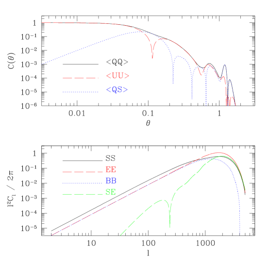
The top panel of figure 1 shows the correlation functions from equation (54), while the bottom panel of the same figure shows the different noise power spectra using a standard CDM temperature power spectrum. The correlations in the CMB derivatives drop significantly for angles larger than $\xi=0.15^{\circ}$. The power spectra shown in figure 1 demonstrate that the large scale behavior of the correlations is like white noise. In the limit of low $l$ we can obtain the power spectrum from equation (63) by integrating over angle first and using the orthonormality relation of the Bessel functions,

$$\lim_{l\rightarrow 0}N_{l}^{{\cal S}{\cal S}} = 2\pi\int\theta d\theta(C_{0}^{2}+C_{2}^{2})/\sigma_{\cal S}^{2}$$ (64)

$$= (2\pi\sigma_{\cal S}^{2})^{-1}\int\theta d\theta\int l^{3}dl\int l^{\prime 3}dl^{\prime}C_{l}^{TT}C_{l^{\prime}}^{TT}[J_{0}(l\theta)J_{0}(l^{\prime}\theta)+J_{2}(l\theta)J_{2}(l^{\prime}\theta)]$$ (65)

$$= {1\over\pi}\ \ {\int l^{5}dl(C_{l}^{TT})^{2}\over(\int l^{2}dlC^{TT}_{l})^{2}}$$ (66)

$$\lim_{l\rightarrow 0}N_{l}^{{\cal E}{\cal E}} = 2\pi\int\theta d\theta C_{0}^{2}/\sigma_{\cal S}^{2}=\lim_{l\rightarrow 0}N_{l}^{{\cal B}{\cal B}}={1\over 2}\lim_{l\rightarrow 0}N_{l}^{{\cal S}{\cal S}}$$ (67)

$$\lim_{l\rightarrow 0}N_{l}^{{\cal S}{\cal E}} = 0.$$ (68)

We can use these to define the correlation length more precisely as $\xi^{2}=N_{l}^{\cal SS}$ which gives $\xi\sim 0.15^{\circ}$ used above. It is interesting to note that although ${\cal S}$, ${\cal Q}$, ${\cal U}$ all have the same variance the power spectrum of $\cal S$ is twice that of $\cal E$ or $\cal B$. $\cal E$ and $\cal B$ have a different correlation length from $\cal S$, which reflects the spin nature of the shear variables. This leads to $\cal E$ giving a factor of 2 higher signal to noise than $\cal S$ in the reconstruction.

In order to get an accurate measurement of the projected mass density or the shear we need to average over several “independent” patches of size $\xi^{2}$, each of which has a variance of order unity. This sets the basic requirement that has to be satisfied if the reconstruction is to give a positive signature. The signal to noise in each patch of size $\xi^{2}$ is $S/N\sim 2\kappa$. This means that we need to average over $N_{patch}^{-1/2}\sim 2|\kappa|$ to get a signal to noise of order one. The issue is whether on scales larger than $\xi$ the weak lensing signal is sufficiently strong to be detectable. Even though CMB is sensitive to matter density fluctuations up to $z\sim 1100$ and the RMS convergence is significantly higher than for galaxies at say $z\sim 1$, it is still well below the CMB noise if $\xi=0.15^{\circ}$. Only with sufficient small scale power can individual structures be reconstructed with high enough signal to noise. This is discussed further in the following sections.

FIG. 1.: The upper panel shows the correlation function of $\tilde{S}$, $\tilde{Q}$, $\tilde{U}$ for SCDM. The lower panel shows the power spectra of $\cal SS$, $\cal EE$, $\cal BB$ and $\cal SE$.

Equations (63) are needed to asses the noise for the reconstruction of $\kappa$ and to subtract the noise contribution to its reconstructed power spectrum in equation (55). To compute the variance of the power spectrum reconstruction we also need to know the RMS of the CMB noise power spectrum. The CMB noise is a fourth order statistics of CMB field. Fortunately in the large scale limit it can be considered Gaussian. This is a consequence of the central limit theorem: the long wavelength modes of ${\cal S}$, ${\cal E}$ and ${\cal B}$ are obtained by adding a lot of independent patches making them effectively Gaussian.

If the CMB noise can be considered Gaussian then the covariance matrix ${\rm Cov}(XX^{\prime})$ for the noise power spectra can be expressed in terms of these [14],

$${\rm Cov}[(N^{\cal SS}_{l})^{2}] = {2\over 2l+1}(N^{\cal SS}_{l})^{2}$$ (69)

$${\rm Cov}[(N^{\cal EE}_{l})^{2}] = {2\over 2l+1}(N^{\cal EE}_{l})^{2}$$ (70)

$${\rm Cov}[(N^{\cal SE}_{l})^{2}] = {1\over 2l+1}[(N^{\cal SE}_{l})^{2}+N^{\cal SS}_{l}N^{\cal EE}_{l}]$$ (71)

$${\rm Cov}(N^{\cal SS}_{l}N^{\cal EE}_{l}) = {2\over 2l+1}(N^{\cal SE}_{l})^{2}$$ (72)

$${\rm Cov}(N^{\cal SS}_{l}N^{\cal SE}_{l}) = {2\over 2l+1}N^{\cal SE}_{l}N^{\cal SS}_{l}$$ (73)

$${\rm Cov}(N^{\cal EE}_{l}N^{\cal SE}_{l}) = {2\over 2l+1}N^{\cal SE}_{l}N^{\cal EE}_{l}.$$ (74)

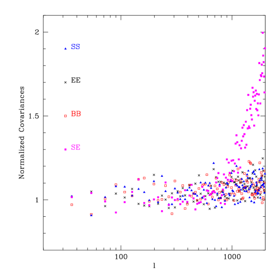
In the large scale limit $N^{\cal SE}_{l}\ll N^{\cal EE}_{l}$ and $N^{\cal SS}_{l}=2N^{\cal EE}_{l}=2N^{\cal BB}_{l}$. The covariance matrix becomes diagonal with ${\rm Cov}[(N^{\cal EE}_{l})^{2}]={\rm Cov}[(N^{\cal BB}_{l})^{2}]={\rm Cov}[(N^{\cal SE}_{l})^{2}]={\rm Cov}[(N^{\cal SS}_{l})^{2}]/4$. In figure 2 the covariances obtained in the simulations are compared to those derived under the Gaussian approximation. The agreement is excellent for $l<1000$ and only seriously breaks down beyond that for $N^{\cal SE}$. We have also verified with Monte Carlo simulations that the off-diagonal terms are negligible compared to the diagonal ones.

In equation (55) we have three estimators for the convergence power spectrum, ${\cal SS}$, ${\cal EE}$ and the cross correlation ${\cal SE}$. Using the covariance matrix in (74) we can construct a minimum variance combination of the three estimators. In the large scale limit the covariance matrix is diagonal and we can weight each of the estimators by the inverse of noise variance,

$$4\hat{C}^{\kappa\kappa}_{l} = {1\over 9}(C_{l}^{\cal S\cal S}-N_{l}^{\cal S\cal S})+{4\over 9}(C_{l}^{\cal E\cal E}-N_{l}^{\cal E\cal E})+{4\over 9}(C_{l}^{\cal S\cal E}-N_{l}^{\cal S\cal E})$$ (75)

Note that we have assumed in equation (74) that only the CMB noise contributes to the variance of $C_{l}^{\kappa\kappa}$ estimates. There is also the cosmic variance contribution ${2\over 2l+1}(C_{l}^{\kappa\kappa})^{2}$ but we will be show in the following sections that this term is significantly smaller than the CMB noise term and can be ignored, unless the CMB has more small scale power than expected within the currently popular cosmological models.

FIG. 2.: Simulation results for the covariances of $N_{l}^{\cal SS}$, $N_{l}^{\cal EE}$ $N_{l}^{\cal BB}$ and $N_{l}^{\cal SE}$ normalized to their values for Gaussian noise given in equation (74). The Gaussian approximation is an excellent one for $l<1000$.

B Small Scale Limit

So far we have described the gravitational lensing effect on large scales compared to the correlation length of the CMB. In this limit we average over (almost) independent patches of CMB fluctuations, which is similar to the procedure used in weak lensing, where we average over independent ellipticities of background galaxies. We now turn to scales much smaller than the correlation length $\xi$. In this limit we can take the derivatives $\tilde{T}_{x}$ and $\tilde{T}_{y}$ to be constant across the field. The physical picture is very different from the one discussed in previous subsection. Weak lensing in this limit acts as a generator of small scale power. To see this we can imagine the effect of a small clump of mass on a pure gradient of temperature field. A mass clump will magnify and stretch a small patch, which will change the slope of the gradient at the position of the clump. The resulting temperature field is no longer a pure gradient, but has a small wiggle superimposed on it. Small scale power has been generated only where the gradient of primary anisotropies is non-zero because where the surface brightness is constant its conservation requires that it remains so even in the presence of lensing.

We now attempt to use this physical picture to reconstruct the weak lensing signal. Introducing $a=T_{x}/\sigma_{\cal S}$ and $b=T_{y}/\sigma_{\cal S}$ we have

$${\cal S} = (2\kappa-1)(a^{2}+b^{2})+2\gamma_{1}(a^{2}-b^{2})+2\gamma_{2}\ 2ab$$ (76)

$${\cal Q} = (2\kappa-1)(a^{2}-b^{2})+2\gamma_{1}(a^{2}+b^{2})$$ (77)

$${\cal U} = (2\kappa-1)2ab+2\gamma_{2}(a^{2}+b^{2}).$$ (78)

We did not subtract unity out of the definition of $S$ as in equation (27), because even though on average $\langle(a^{2}+b^{2})\rangle_{CMB}=1$, we are considering a very small field over which $a$ and $b$ are approximately constant with $(a^{2}+b^{2})\neq 1$ in general.

We want to determine $a$, $b$, $\kappa$, $\gamma_{1}$ and $\gamma_{2}$. If we assume that the mean value of $\kappa$, $\gamma_{1}$ and $\gamma_{2}$ over the field is zero then

$$\langle{\cal S}\rangle = a^{2}+b^{2}$$ (79)

$$\langle{\cal Q}\rangle = a^{2}-b^{2}$$ (80)

$$\langle{\cal U}\rangle = 2ab,$$ (81)

where the mean value is taken over a region large enough that the mean shear and projected mass density vanish but over which the CMB gradient remains nearly constant. In practice this can be achieved by filtering out the small scale power, so that the remaining power is largely dominated by primary anisotropies. We can then compute $a$ and $b$ and use them in equation (81).

Once $a$ and $b$ are determined it would appear that we can determine the convergence and the two shear components by solving

$$\left(\begin{array}[]{c}{\cal S}\\ {\cal Q}\\ {\cal U}\end{array}\right)=\left(\begin{array}[]{c c c}\langle{\cal S}\rangle&\langle{\cal Q}\rangle&\langle{\cal U}\rangle\\ \langle{\cal Q}\rangle&\langle{\cal S}\rangle&0\\ \langle 0\rangle&\langle{\cal U}\rangle&\langle{\cal S}\rangle\\ \end{array}\right)\ \left(\begin{array}[]{c}1-2\kappa\\ -2\gamma_{1}\\ -2\gamma_{2}\end{array}\right).$$ (82)

However, the determinant of the matrix above vanishes so we cannot determine convergence and shear independently. Instead we have to use the relations between shear and convergence to reconstruct the signal. In Fourier space, for $l$ large enough that we can consider $a$ and $b$ in equation (78) as constants. We get,

$${\cal S}(\hbox{\boldmath{$l$}}) = 2\kappa({\hbox{\boldmath{$l$}}})\left[(a^{2}+b^{2})+(a^{2}-b^{2})\cos(2\phi_{\hbox{\boldmath{$l$}}})+2ab\sin(2\phi_{\hbox{\boldmath{$l$}}})\right]$$ (83)

$${\cal Q}(\hbox{\boldmath{$l$}}) = 2\kappa(\hbox{\boldmath{$l$}})\left[(a^{2}-b^{2})+(a^{2}+b^{2})\cos(2\phi_{\hbox{\boldmath{$l$}}})\right]$$ (84)

$${\cal U}(\hbox{\boldmath{$l$}}) = 2\kappa(\hbox{\boldmath{$l$}})\left[2ab+(a^{2}+b^{2})\sin(2\phi_{\hbox{\boldmath{$l$}}})\right].$$ (85)

We can compute ${\cal E}$ and ${\cal B}$,

$${\cal E}(\hbox{\boldmath{$l$}}) \equiv {\cal Q}(\hbox{\boldmath{$l$}})\cos(2\phi_{\hbox{\boldmath{$l$}}})+{\cal U}(\hbox{\boldmath{$l$}})\sin(2\phi_{\hbox{\boldmath{$l$}}})$$ (86)

$$= 2\kappa(\hbox{\boldmath{$l$}})\left[(a^{2}+b^{2})+(a^{2}-b^{2})\cos(2\phi_{\hbox{\boldmath{$l$}}})+2ab\sin(2\phi_{\hbox{\boldmath{$l$}}})\right]$$ (87)

$$= {\cal S}(\hbox{\boldmath{$l$}})$$ (88)

$${\cal B}(\hbox{\boldmath{$l$}}) \equiv {\cal U}(\hbox{\boldmath{$l$}})\cos(2\phi_{\hbox{\boldmath{$l$}}})-{\cal Q}(\hbox{\boldmath{$l$}})\sin(2\phi_{\hbox{\boldmath{$l$}}})$$ (89)

$$= 2\kappa(\hbox{\boldmath{$l$}})\left[2ab\cos(2\phi_{\hbox{\boldmath{$l$}}})+(a^{2}-b^{2})\sin(2\phi_{\hbox{\boldmath{$l$}}})\right].$$ (90)

We see that the estimators of the convergence are not independent, ${\cal E}(\hbox{\boldmath{$l$}})={\cal S}(\hbox{\boldmath{$l$}})$, as argued above.

To obtain an estimator of convergence we can use any of the expressions in equation (85). This requires dividing with the combination of derivatives of $T$ and will be very noisy if both $a$ and $b$ are close to 0. This is a consequence of the fact that lensing cannot generate power where there is no gradient. Such a reconstruction will therefore have variable noise. One solution to this problem is to filter the map with a variable filtering length. Note that we have assumed $a$ and $b$ are constant across the map, while in reality they will change as well. This means that in practice we have to divide the map into chunks over which the long wavelength modes are approximately constant, or use more sophisticated methods such as the wavelet analysis.

The procedure outlined above is quite involved and we did not attempt to implement it in this paper. It simplifies considerably if we are only interested in the power spectrum. In this case we may still use ${\cal S}(\hbox{\boldmath{$l$}})$ and ${\cal B}(\hbox{\boldmath{$l$}})$ to get,

$$C^{\cal SS}_{\hbox{\boldmath{$l$}}} = 4C^{\kappa\kappa}_{l}\left[(a^{2}+b^{2})^{2}+(a^{2}-b^{2})^{2}\cos^{2}(2\phi_{\hbox{\boldmath{$l$}}})+(2ab)^{2}\sin^{2}(2\phi_{\hbox{\boldmath{$l$}}})\right.$$ (91)

$$+ \left.2(a^{2}+b^{2})(a^{2}-b^{2})\cos(2\phi_{\hbox{\boldmath{$l$}}})+4(a^{2}+b^{2})ab\sin(2\phi_{\hbox{\boldmath{$l$}}})+4(a^{2}-b^{2})ab\cos(2\phi_{\hbox{\boldmath{$l$}}})\sin(2\phi_{\hbox{\boldmath{$l$}}})\right]$$ (92)

$$C^{\cal BB}_{\hbox{\boldmath{$l$}}} = 4C^{\kappa\kappa}_{l}\left[+(2ab)^{2}\cos^{2}(2\phi_{\hbox{\boldmath{$l$}}})+(a^{2}-b^{2})^{2}\sin^{2}(2\phi_{\hbox{\boldmath{$l$}}})\right.$$ (93)

$$- \left.4(a^{2}-b^{2})ab\cos(2\phi_{\hbox{\boldmath{$l$}}})\sin(2\phi_{\hbox{\boldmath{$l$}}})\right].$$ (94)

If we average over $\phi_{\hbox{\boldmath{$l$}}}$ and use $\langle(a^{2}+b^{2})^{2}\rangle_{CMB}=\langle\tilde{T}_{x}^{4}+\tilde{T}_{y}^{4}+2\tilde{T}_{x}^{2}\tilde{T}_{y}^{2}\rangle_{CMB}/\sigma_{\cal S}^{2}=2$ and $\langle(a^{2}-b^{2})^{2}\rangle_{CMB}=\langle(2ab)^{2}\rangle_{CMB}=1$ we find,

$$C^{\cal SS}_{l} = 12C^{\kappa\kappa}_{l}$$ (95)

$$C^{\cal BB}_{l} = 4C^{\kappa\kappa}_{l}.$$ (96)

Note that there is no need to use local estimates of $a$ and $b$ to get an estimator of the power spectrum, as long we have a CMB map with enough uncorrelated patches so that the quadratic combinations of $a$ and $b$ can be replaced by their averages. In this limit the power spectra of ${\cal S}$ and ${\cal B}$ again directly give estimates of convergence power spectrum, without any convolution and also without noise contribution from intrinsic CMB anisotropies (although there will be contribution from instrumental noise). This is because in this limit all the power is generated by gravitational lensing. It is important to note that in this limit $\cal B$ does not vanish, but actually gives an estimate of the $\kappa$ power spectrum, while power in ${\cal S}$ is a factor of $3$ bigger than power in ${\cal B}$. We will show below that these predictions are well recovered in the Monte Carlo simulations.

III Reconstructing the mass profile of a cluster

To illustrate our method we first apply it to reconstruct the mass profile of a massive cluster of galaxies. In order for the large scale limit method to work we need the CMB to vary on scales smaller than the cluster, so that the effect of lensing can be measured after averaging over independent patches. Since we do not expect the primary CMB anisotropies to have sufficient power on arcminute scales we use the Ostriker-Vishniac (OV) effect instead in our example using the power spectrum from [17] as an estimate. This is not necessary the only possible source of anisotropies on small scales and there may be other sources as well, including the primeval galaxies and QSO emitting in IR and radio. As long as there are many sources in the beam and their redshift is higher than the cluster redshift the analysis is identical to the one presented here. The only difference is that these sources are not at $z\sim 1100$ but at lower redshift so the window function $g$ in equation (9) changes relative to the one for $z\sim 1100$ sources. If the redshift distribution of the sources is not known then we may in principle use lensing on a cluster with known mass profile to determine it. For individual sources that are resolved it may be better to use their shapes as an estimate of the local shear, which is the usual procedure in the case of galaxy lensing.

For the method to be useful in practice the small scale anisotropies have to be above the detector noise. This could be achievable with future interferometric or bolometer experiments with long integration times on a small area of the sky, reaching $\mu K$ sensitivities on subarcminute pixels. Another complication in this case relative to our analysis in §2 is that the distribution of anisotropies is likely not to be Gaussian. This complicates the issue of noise analysis and statistical significance of the results, but does not affect the average of the reconstruction. We will ignore these issues in the following, since we are mainly interested in having a simple example with which we can test our method.

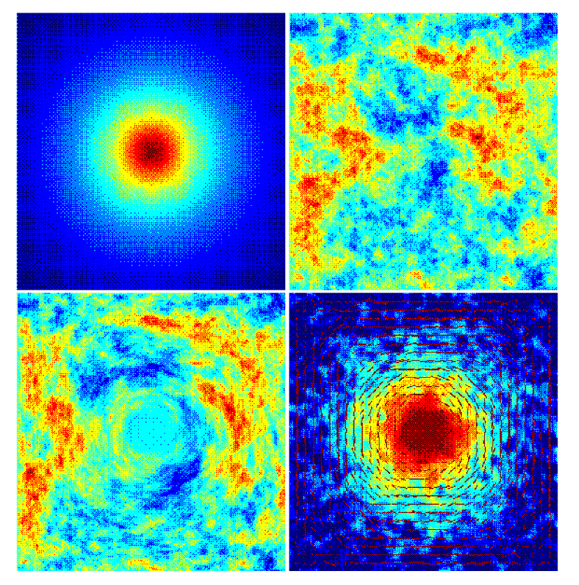
Figure 3a shows the simulated input cluster, with the profile chosen as a projection of a truncated isothermal sphere. In figure 3b we show an unlensed simulated CMB field, assuming OV type of power spectrum. In figure 3c we show the lensed CMB map. We see that the cluster has magnified the CMB in the center, so in the absence of small scale power the central region is smoother. In figure 3d we show the shear as measured by the CMB derivatives ($\cal Q$ and $\cal U$) and in the background the convergence field $\cal S$.

Both $\cal S$ and $\cal E$ are estimators of the convergence, but figure 3c illustrates a possible advantage of the reconstruction based on shear over that based on ${\cal S}$ in the case of clusters. The shear based reconstruction is nonlocal as shown from equation (34). The shear from the whole map is used to reconstruct the density at the center. Thus we are averaging over many different independent CMB regions. On the other hand the reconstruction based on ${\cal S}$ is local. It will not work very well in the center because the magnification induced by the lensing will expand a small region so unless there are additional small scale perturbations which are magnified there will be fewer independent regions to average over. This effect can be seen in figure 3c. This is of course an issue only for clusters that are close to being critical and the magnification is no longer small compared to unity. For other, more linear structures the two reconstructions give similar results, although $\cal S$ is still noisier than $\cal E$ by a factor of 2 as derived in equation (68).

FIG. 3.: Top left panel: input cluster on a 6’$\times$6’ field. Top right panel: unlensed CMB map. We assumed that the Ostriker-Vishniac effect could be detected with sufficient signal to noise to be used in the reconstruction of $\kappa$. Bottom left: CMB field after being lensed by the cluster. Bottom right: the background shows the $\cal S$ field while the rods represent the shear variables ${\cal Q}$ and ${\cal U}$, both of which can be used to reconstruct the density profile.

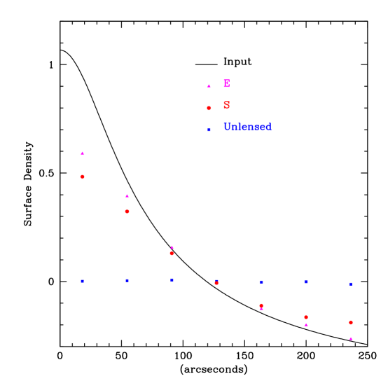
To be more quantitative we show in figure 4 the reconstructed projected radial mass profile from the shear and the convergence. We also show the result of the reconstruction procedure on the unlensed CMB field to illustrate the noise level, which for this case with a lot of small scale structure is negligible. The reconstructed profile tracks well the input profile outside the center, but falls below it in the center because of insufficient number of independent patches there. In our reconstruction algorithm we are forcing the mean $\kappa$ to be zero and because the reconstruction of the center of the cluster is systematically lower due to the averaging, the reconstruction is also systematically lower on the outside of the cluster. As expected this is more pronounced for ${\cal S}$ than for ${\cal E}$ reconstruction because the former is noisier and relies more on poor quality information from the center of the cluster. These effects can be calibrated from the simulations and overall the method can reconstruct the true projected mass density outside the core, assuming that the necessary conditions discussed above (measurable primary anisotropies on scales smaller than the typical cluster scale) are satisfied.

FIG. 4.: Reconstructed radial profile using the data in Figure 2. The points marked with ${\cal E}$ (${\cal S}$) correspond to the reconstruction of $\kappa$ based on ${\cal E}$ (${\cal S}$). The points marked unlensed correspond to the result of applying the ${\cal E}$ reconstruction to the unlensed field. The input $\kappa$ was taken to have zero mean.

IV Reconstructing the power spectrum of projected density

A CMB Noise

In this section we investigate the power spectrum reconstruction of convergence using the method developed in §2. The power spectrum can be reconstructed from ${\cal E}$, ${\cal S}$ or their cross correlation. We will first discuss the power spectrum reconstruction in the absence of detector noise and assuming infinite angular resolution. In this simplified case the only source of noise is the CMB itself. We do not add small scale secondary anisotropies in this section, so the results should be representative for primary fluctuations and any additional small scale fluctuations at high redshift would further improve the performance. In figure 5a we show the power spectra for the unlensed CMB field (the CMB “noise”) calculated using equation (63) and the result of our Monte Carlo simulations. The agreement between analytic prediction and simulations is very good. We recover the white noise behavior of $N^{\cal SS}_{l}$,$N^{\cal EE}_{l}$ and $N^{\cal BB}_{l}$ on large scales and also the relatively small amplitude of the cross correlation $N^{\cal SE}_{l}$.

FIG. 5.: (a) $N^{\cal SS}_{l}$, $N^{\cal EE}_{l}$, $N^{\cal BB}_{l}$ and $N^{\cal SE}_{l}$ power spectra for the unlensed CMB field. The lines correspond to the results of equation (63). Also shown is the weighted average of the recovered power spectra from ${\cal S}$, ${\cal E}$ and their cross correlation together with the input $4C^{\kappa\kappa}_{l}$. (b) Ratio of the recovered power spectra to the input $C^{\kappa\kappa}_{l}$. The signal in ${\cal B}$ is also shown.

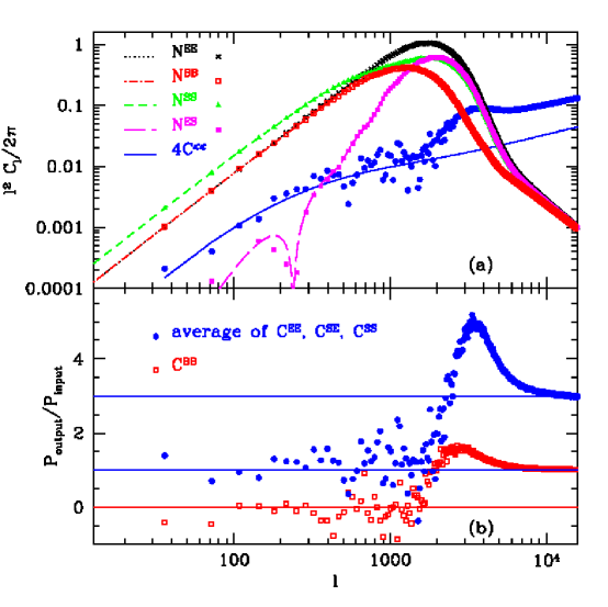
On large scales these power spectra are to be compared to $4C_{l}^{\kappa\kappa}$ (figure 5a). For the purpose of illustrating our method in this paper we adopted the convergence power spectra of the “concordance” model [20] $\Omega_{m}=0.3$, $\Omega_{\Lambda}=0.7$, $\Gamma=\Omega_{m}h=0.2$, $n=1$ and $\sigma_{8}=1$. It can be seen from figure 5a that on large scales the power of the convergence is small compared to that of the CMB noise. As a result we can only hope for a statistical detection of the lensing effect and the method will not allow to make a map of $\kappa$ directly unless there is more small scale power in the CMB, as discussed in §3 in the context of cluster reconstruction. Even if $\kappa$ reconstruction has a low signal to noise its power spectrum may nevertheless be recovered with high statistical significance, because we can average over many independent patches on the sky. This is seen from the difference between the power spectra in the lensed and unlensed field. The weighted average of the three estimators (equation 75) is also shown in figure 5a together with the input convergence spectrum. The intrinsic CMB noise is about 10-20 times higher, yet the difference agrees well with the input $\kappa$ power spectrum, showing that there is a significant statistical detection of the signal.

The reconstruction of the power spectrum is further studied in figure 5b, where we show the CMB noise subtracted power spectra of ${\cal SS}$, ${\cal EE}$ and ${\cal BB}$ and the cross correlation spectrum ${\cal SE}$ divided with the input matter power spectrum. On large scales the reconstructed spectra of $\cal SS$, $\cal EE$ and $\cal SE$ all give unbiased estimators of $4C_{l}^{\kappa\kappa}$ so the average of the output to input ratio is 1, while that of $\cal BB$ if consistent with the pure noise and the ratio averages to 0. The latter, although not giving an estimate of the signal, can provide an important consistency check on whether the signal seen from ${\cal E}$ and ${\cal S}$ is indeed of cosmological origin or not. It may also help identify the cosmological part of the signal if additional contributions are present, such as in the case of non Gaussian CMB fluctuations or contamination from foregrounds.

The large scale limit is valid up to $l\sim 1000$. On very small scales, roughly $l\sim 5000$ and beyond, the reconstructed power spectra from ${\cal E}$ and ${\cal S}$ give $12C^{\kappa\kappa}_{l}$, while that obtained from ${\cal B}$ gives $4C^{\kappa\kappa}_{l}$ so that the ratios are 3 and 1, again in agreement with analytic prediction in equation (96). At very high $l$ CMB noise is negligible, because there is no power present in the CMB itself on those scales.

In the intermediate regime between $l=1000-5000$ neither small scale nor large scale limits apply and the reconstruction becomes a complicated convolution of CMB anisotropies and lensing signal. Information on the power spectrum can still be obtained even from this regime, but it is better to approach the reconstruction in a parametric form, by parameterizing the power spectrum with a few free parameters that can be estimated by fitting the simulated spectra to the data, rather than by direct inversion.

Because CMB noise is larger than the signal on large scales we may worry that a small error in the noise estimate would lead to a large error in the estimated power spectrum. This is most worrisome for the ${\cal SS}$ reconstruction and least important for the cross correlation ${\cal SE}$ because $N_{l}^{\cal SS}=2N_{l}^{\cal EE}\gg N_{l}^{\cal SE}$. The latter is even smaller than $4C_{l}^{\kappa\kappa}$ on large scales so we can obtain an accurate estimate even without any noise subtraction. Fortunately the large scale behavior of $N_{l}^{\cal SS}$, $N_{l}^{\cal EE}$ $N_{l}^{\cal BB}$ and $N_{l}^{\cal SE}$ is quite insensitive to the details of the power temperature spectra. For example we may worry that the CMB power spectra we measure will be affected by lensing or that we can only know the lensed CMB temperature spectra with some minimum scatter, limited by cosmic variance. On large scales, these effects change the mean of $N_{l}^{\cal EE}$ by approximately 0.5 % and add a 1% scatter to it. It will depend on the noise amplitude whether this is a significant source of error. For MAP these errors causes a shift in the amplitude comparable to the input power spectrum, while for Planck it is significantly below it and can be ignored. For MAP this problem can be solved by using $\cal B$ reconstruction. Because the effect on large scales is mostly an amplitude shift we may use the amplitude of $C^{\cal BB}_{l}$ to make it consistent with 0, which would also properly determine the amplitude of the other spectra.

B Finite Angular Resolution and Detector Noise

Next we consider the influence of finite angular resolution and detector noise. In order to measure the convergence power spectra using the small scale limit the experiment must have enough angular resolution to probe these small scales. This effect of finite angular resolution is straightforward to include and we will not discuss it further, because future CMB satellites such as MAP and Planck will not be able to probe this limit. Here we discuss the more important effect of finite angular resolution and detector noise on the large scale limit reconstruction. It is easy to see that finite angular resolution has an effect on the intrinsic CMB noise amplitude. Because of finite resolution and detector noise small scale CMB power cannot be resolved and this leads to a larger correlation length $\xi$. This means that we have fewer independent patches to average over the CMB noise and the overall level of noise power spectrum is higher. Finite angular resolution also has a more subtle effect by reducing the transfered power. To understand it quantitatively we first compute the derivatives of the temperature field in the presence of some filtering function $F({\hbox{\boldmath{$\theta$}}})$, which involves the experimental beam and any additional filter we may want to use in the analysis

$$T_{a}({\hbox{\boldmath{$\theta$}}}) = \int F(\hbox{\boldmath{$\theta$}}-\hbox{\boldmath{$\theta$}}^{\prime})T_{a}(\hbox{\boldmath{$\theta$}}^{\prime})d^{2}{\hbox{\boldmath{$\theta$}}}^{\prime}$$ (97)

$$= \int F(\hbox{\boldmath{$\theta$}}-\hbox{\boldmath{$\theta$}}^{\prime})(\delta_{ab}+\Phi_{ab}){\tilde{T}}_{b}(\hbox{\boldmath{$\theta$}}^{\prime}+\delta{\hbox{\boldmath{$\theta$}}}^{\prime})d^{2}{\hbox{\boldmath{$\theta$}}}^{\prime}$$ (98)

$$= (2\pi)^{-2}\int d^{2}{\hbox{\boldmath{$l$}}}F(l)T_{a}({\hbox{\boldmath{$l$}}})e^{i{\hbox{\boldmath{$l$}}}\cdot\hbox{\boldmath{$\theta$}}}$$ (99)

$$+ (2\pi)^{-4}\int d^{2}{\hbox{\boldmath{$l$}}}\int d^{2}{\hbox{\boldmath{$q$}}}F(|\hbox{\boldmath{$l$}}+\hbox{\boldmath{$q$}}|)T_{b}({\hbox{\boldmath{$l$}}})\Phi_{ab}(\hbox{\boldmath{$q$}})e^{i{(\hbox{\boldmath{$l$}}+\hbox{\boldmath{$q$}})}\cdot\hbox{\boldmath{$\theta$}}}.$$ (100)

To obtain the last expression we expanded $F$, $\Phi_{ab}$ and $T_{a}$ into a Fourier series and integrated over angle ${\hbox{\boldmath{$\theta$}}}^{\prime}$. The large scale effect of the filter function can be read from the average over CMB of the square of equation (100),

$$\langle T_{a}T_{b}\rangle_{CMB} = {\delta_{ab}\over 2}\int{ldl\over 2\pi}\ F^{2}(l)l^{2}C^{TT}_{l}$$ (101)

$$+ (2\pi)^{-2}\int d^{2}{\hbox{\boldmath{$q$}}}\Phi_{ab}(\hbox{\boldmath{$q$}})e^{i{\hbox{\boldmath{$q$}}}\cdot\hbox{\boldmath{$\theta$}}}\left[(2\pi)^{-2}\int d^{2}{\hbox{\boldmath{$l$}}}F(l)F(|\hbox{\boldmath{$l$}}+\hbox{\boldmath{$q$}}|)C^{TT}_{l}\right]$$ (102)

In the absence of filtering the integrals involving $C^{TT}_{l}$ in both terms of equation (102) are identical. This allows us to reconstruct $\kappa$ from the second term, while the first term gives $\sigma_{\cal S}$ as in equation (24). To describe the effect of the beam smearing we introduce a window function as the ratio of the two integrals

$$W(q)={\int d^{2}{\hbox{\boldmath{$l$}}}F(l)F(|\hbox{\boldmath{$l$}}+\hbox{\boldmath{$q$}}|)l^{2}C^{TT}_{l}\over\int d^{2}{\hbox{\boldmath{$l$}}}\ F^{2}(l)l^{2}C^{TT}_{l}},$$ (103)

which is in general less than unity and in terms of which we have

$$\langle{\cal S}({\hbox{\boldmath{$l$}}})\rangle=\langle{\cal E}({\hbox{\boldmath{$l$}}})\rangle=2\kappa({\hbox{\boldmath{$l$}}})W(l).$$ (104)

The effect of filtering is important even for the reconstruction of large scale $\kappa$ modes. This can be understood by looking at equation (100). The shear tensor modulates the amplitude of the temperature derivatives, so the information about a particular $q$ mode of $\kappa$ is encoded as sidebands of the different $l$ modes of the temperature. We are recovering the information back at the corresponding $q$ by squaring the field, which appropriately combines back all the sidebands from every $l$ to the correct $q$. Finite angular resolution is important even for large scale modes because the information about these modes in encoded mainly in the sidebands of the small scale temperature modes, which are strongly affected by the filtering function.

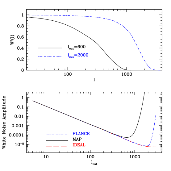
To minimize the effect of beam smoothing we may filter the temperature before squaring it. The smallest effect is achieved if the filtering function $F(l)$ is a constant, in which case (in the absence of a cutoff in $l$) there would be no effect. For this reason we choose to filter the temperature with the inverse of the beam $e^{l(l+1)\sigma_{b}^{2}}$, where $\sigma_{b}^{2}$ is the width of the Gaussian beam, thereby reversing the smoothing effect of the beam. We can only do this up to a maximum $l_{cut}$ (the value of which is determined below) not to amplify the detector noise on small scales. Thus our effective filter $F(l)$ is equal to one for $l<l_{cut}$ and zero after that. Figure 6a shows two examples of $W(q)$ for different values of $l_{cut}$, which correspond to minimum of noise for MAP and Planck experiments. Note that regardless of the form of the filter equation (103) implies that $W(q)\rightarrow 1$ as $q\rightarrow 0$. Other forms of filtering are possible as well, but we show next that this filter comes close to being optimal and is easy to implement in the analysis.

The contribution of detector noise on large scales to the different power spectra can be obtained using equation (63) with $C^{TT}_{l}\rightarrow C_{l}^{TT}+N^{TT}$. We take the detector noise to be white noise with constant power spectrum $N^{TT}$ for a range $0<l<l_{max}$. The power spectrum $N^{TT}$ is related to the noise level per pixel, $\sigma^{2}=N^{TT}l_{max}^{2}/4\pi$ with $l_{max}^{2}=N_{pix}4\pi/\Omega$ and $\sigma$ is expressed in the same units as $T$ (e.g. $\mu K$). If we want the correct normalization for the recovered $C^{\kappa\kappa}_{l}$ we need to divide by the correct $\sigma_{\cal S}$, which has to be computed only with the CMB power spectrum, without the detector noise term. With our filtering prescription the large scale amplitude of the $N^{\cal EE}_{l}$ power spectrum in equation (68) becomes

$$N^{\cal EE}_{l}=2\pi{\int_{0}^{lcut}ldll^{4}F(l)^{4}(C_{l}^{TT}+e^{l(l+1)\sigma_{b}^{2}}N^{TT})^{2}\over(\int ldll^{2}F^{2}(l)C^{TT}_{l})^{2}}.$$ (105)

To derive the optimal filter $F(l)$ we minimize $N^{\cal EE}_{l}/W^{2}(l)C^{\kappa\kappa}_{l}$ with respect to $F^{2}(l)$. In the limit $l\rightarrow 0$ $W(l)=1$ and this becomes equivalent to minimizing $N^{\cal EE}_{l}$ in equation (105). Taking derivatives with respect to $F(l)^{2}$ and setting to 0 we find

$$F(l)^{2}={C_{l}^{TT}\over l^{2}(C_{l}^{TT}+e^{l(l+1)\sigma_{b}^{2}}N^{TT})^{2}}.$$ (106)

In the large scale limit this gives $F(l)^{2}=(l^{2}C_{l}^{TT})^{-1}$, which is roughly a constant for spectra that are close to scale invariant. For large $l$ the noise term dominates over the CMB signal term and the filtering function $F(l)$ goes to 0. The transition occurs where

$$C_{l}^{TT}\sim e^{l(l+1)\sigma_{b}^{2}}N^{TT}.$$ (107)

To compare this filter to the simple constant filter in figure 6b we show $N^{\cal EE}_{l}$ as a function of $l_{cut}$ for the constant filter and the specifications of noise and angular resolution of MAP and Planck, as well as in the absence of noise and beam smoothing. In the absence of detector noise larger $l_{cut}$ is always better because the correlation length is reduced, but it saturates beyond $l\sim 2000$ for this model because there is very little CMB power on small scales. Once detector noise is included it eventually dominates at high $l_{cut}$ and we are better off not including these modes as they are mostly noise and do not contribute to the signal. In between there is a minimum which determines $l_{cut}$ depending on the noise and beam of the experiment. The amplitude of noise for this filter can be compared to the one in equation (106) which minimizes the noise in the large scale limit. The two give very similar results in the large scale limit. Because constant $F(l)$ minimizes the effect of the window at higher $l$ it is likely to perform even better than the filter in equation (106), which was derived under assumption $W(l)=1$. For this reason we choose to adopt the simple constant filter instead of the one in equation (106).

FIG. 6.: The upper panel shows the window function $W^{2}(l)$ as a function of $l$ for MAP noise and beam properties where the appropriate value is $l_{cut}=600$ and for Planck with $l_{cut}=2000$ (bottom panel). For the latter the window has no effect at $l<1000$. Bottom panel shows amplitude of $N^{\cal EE}_{l}$ in the limit $l\rightarrow 0$ as a function of $l_{cut}$ for the specifications of the MAP and Planck satellites, justifying $l_{cut}=600,2000$ for the two experiments. Also shown is the no noise infinite angular resolution curve (Ideal), which levels off at $l\sim 2000$, showing that Planck is close to optimal in the large scale limit, because it measures most of the power in the CMB.

C Relation to the Density Field

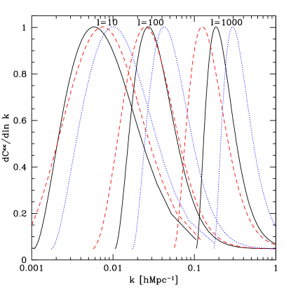
We have shown that the quantity we are able to extract from the distortions of the CMB is the power spectrum of the projected density field weighted with a window $g/a$ (equation 9). Since the more fundamental quantity is the 3-d density field described by the power spectrum we would like to know the relation between the two power spectra. This relation is shown in figure 7a, where a logarithmic contribution to a given $l$ mode as a function of 3-d wavevector $k$ is plotted for a representative sample of models. These windows are relatively broad functions of $k$ and peak at $\lambda=2\pi/k=1000h^{-1}$Mpc for $l=10$ and $\lambda=30h^{-1}$Mpc for $l=1000$. The exact value depends on the model. We are therefore probing the power spectrum over a range of scales which extends to scales larger than any other method that directly traces dark matter.

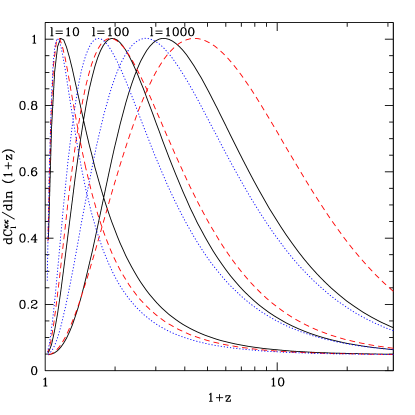
The next question we want to address is the redshift distribution of the contribution to a given $C_{l}^{\kappa\kappa}$. Even though the $g/a$ window peaks at $z=3$ for a flat universe this does not mean that the dominant contribution comes from this redshift. The relation between $l$ and $k$ depends on the shape of the power spectrum (equation 10). For any given $l$ there is a range in $k$ that contributes (figure 7a). The contribution from a high $k$ mode comes from structures which are relatively closer to the observer (and so at lower $z$) than the structures that dominate the contribution for a lower $k$ mode (equation 10). On large scales the matter power spectrum has a turnover so low $k$ modes have very little power which implies that their contribution is smaller than that of higher $k$ modes from more nearby structures despite the geometrical factor that suppresses these higher $k$ modes. Thus for low $l$ the contribution will be dominated by low $z$ structures. The logarithmic contribution to a given $l$ mode as a function of $1+z$ is shown in figure 7b and confirms these expectations. At smaller scales the power is more evenly distributed as a function of $k$ and the peak contribution moves to higher redshifts. For $l\sim 1000$ it peaks between $z\sim 2-3$ with a long tail extending to higher $z$. At these scales we are therefore directly probing dark matter clustering at high redshifts.

FIG. 7.: Left: logarithmic contribution to $C^{\kappa\kappa}_{l}$ as a function of $k$ for $l=10$, 100, 1000 (the normalization is arbitrary). The models are flat CDM model (dotted), open CDM model with $\Omega_{m}=0.3$ (dashed) and cosmological constant model with with $\Omega_{m}=0.3$ (solid). All the models have $\Gamma=\Omega_{m}h=0.21$. Right: logarithmic contribution to $C^{\kappa\kappa}_{l}$ as a function of $1+z$ for the same models as above.

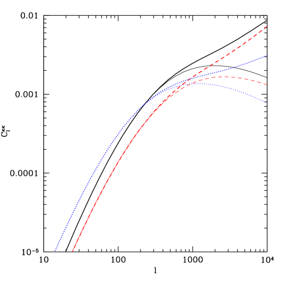
The two characteristic features of lensing on the CMB are the large scales and early epochs we can probe. In combination these facts guarantee that the power spectrum will be dominated by linear contributions. Figure 8 shows the difference between the $C_{l}^{\kappa\kappa}$ calculated using the linear and nonlinear matter power spectrum. The spectra are shown as a function of $l$ for the same set of models used in figure 7. The nonlinear matter power spectra were computed using the linear to nonlinear mapping [21]. Up to $l\sim 1000$ the power spectrum is dominated by linear modes. This has the advantage of making the results simple to interpret in terms of cosmological models, since no nonlinear corrections are necessary. Since MAP and Planck reconstruction in the large scale limit will not extend beyond $l\sim 1000$ they will be dominated by linear scales. At higher $l$ nonlinear corrections become important. While this has the disadvantage that the interpretation becomes more complicated it has the advantage in that the power is boosted by almost an order of magnitude compared to the linear scales and so the lensing effect becomes more easily observable.

FIG. 8.: Power spectrum $C^{\kappa\kappa}_{l}$ as a function of $l$ for the same models as in figure 7. Thin lower curves show the linear power spectra, thick upper curves the nonlinear spectra.

V Cross Correlation with Other Maps

We have shown that individual structures cannot be reconstructed with sufficient signal to noise, unless the CMB has more small scale power than expected from primary anisotropies. One way to obtain a positive detection discussed in previous section is by combining information from independent patches of the sky into a measurement of the power spectrum. In this section we discuss another way to enhance the signal by using the cross correlation with another map with higher signal to noise. A cross correlation between signal induced by lensing and some other tracer has been explored before [22]. The difference to our method is that they do not reconstruct $\kappa$ directly, but compute the photon deflection angle instead for which the 3-d matter distribution is needed. It can only be obtained from a redshift survey (such as SDSS or 2dF), under the assumption that light traces mass. Our method can also be used when such a 3-d distribution is not available. For example, we may try to cross correlate the reconstructed convergence map with Sunyaev-Zeldovich (SZ) map, which traces the integrated pressure along the line of sight. This would give positive cross correlation because of clusters, which should contribute to both convergence and SZ effect. Thus even if clusters cannot be individually detected using the method described in §3, they may still be detected statistically through this cross correlation, which would give information about pressure to dark matter ratio in clusters. Other possibilities for cross correlation are with X-ray background which is believed to trace large scale structure to $z\sim 5$ and with galaxy catalogs from SDSS and 2dF, both of which would give information on how light traces mass on large scales. Yet another possibility is the cross correlation with the CMB itself, which would give positive detection whenever there is a significant contribution from the time-dependent potential in the CMB [13, 23, 24]. To test the most optimistic possibility we may estimate the signal to noise of the cross correlation when we have another perfect map of convergence. For any of the probes mentioned above the actual signal to noise will be lower, since they will only partially correlate with the projected mass density. It is nevertheless of interest to see whether such cross correlations would be useful at all given such a low signal to noise on individual structures in the maps of $\cal S$ and $\cal E$.

FIG. 9.: Cross correlation of the input $\kappa$ and the ${\cal E}$ and ${\cal S}$ statistics. The results correspond to a $100^{\circ}\times 100^{\circ}$ simulation observed with an ideal CMB experiment with negligible detector noise and infinite angular resolution.

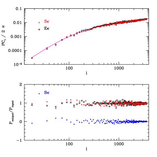
The cross correlations with the input $\kappa$ give

$$C_{l}^{\cal S\kappa} = 2C^{\kappa\kappa}_{l}$$ (108)

$$C_{l}^{\cal E\kappa} = 2C^{\kappa\kappa}_{l}$$ (109)

$$C_{l}^{\cal B\kappa} = 0.$$ (110)

Figure 9 shows the cross correlations in equation (110) for a $100^{o}\times 100^{o}$ field where the CMB is measured with negligible detector noise and infinite angular resolution (the results are almost the same for Planck specifications). The agreement is remarkable, proving that there is enough signal in the $\kappa$ maps recovered using our technique to get useful information about the convergence power spectra by cross correlating them with other maps. This is not surprising, since there are about 5$\times 10^{5}$ independent patches of size $\xi^{2}=(0.15^{\circ})^{2}$ and we need about $(N_{l}^{\cal EE}/4C_{l}^{\kappa\kappa})^{2}\sim 100-400$ of them to obtain signal to noise of unity.

In reality most tracers of the underlying mass will not be perfect because they correlate only partially with $\kappa$. In particular we assume that we have a map $Y$ that correlates with $\kappa$ and has a cross correlation $C^{\kappa Y}_{l}$. Then the cross correlations between the ${\cal W}={\cal S,E}$ maps and the $Y$ map give,

$$C^{{\cal W}Y}_{l} = 2C^{\kappa Y}_{l}W(l)$$ (111)

where $W(l)$ is the window defined in equation (103). The correlation of the $Y$ map with $\cal B$ vanishes, $C^{{\cal B}Y}_{l}=0$. The covariance matrix for the two correlations is,

$${\rm Cov}(C^{\cal W^{\prime}Y}_{l}C^{\cal WY}_{l}) = (C_{l}^{YY}+N_{l}^{YY})(4C_{l}^{\kappa\kappa}W^{2}(l)+N_{l}^{\cal W^{\prime}W})+4C^{\kappa Y}_{l}C^{\kappa Y}_{l}W^{2}(l),$$ (112)

where the first term is usually dominant. Both the decorrelation and the noise reduce the overall signal to noise of the cross correlation. For example, in the case of cross correlation with the CMB only the largest modes are strongly correlated because the time dependent gravitational potential does not contribute to the CMB anisotropies on small scales. The overall signal to noise is significantly reduced compared to the idealized example discussed here, but is nevertheless detectable with future satellite missions for reasonable low density models [13].

VI Conclusions

We have developed a method to reconstruct projected mass density from observed cosmic microwave background maps. The method consists of taking derivatives of temperature field and averaging their products. Particular combinations on average correspond to shear and convergence of gravitational lensing, which can be expressed as a line of sight integral over the density field.

We have presented three possible applications of the method. First we applied the method to simulated clusters showing that it can be successfully used to reconstruct their projected mass distribution if there is sufficient small scale power. For this to be successful we require small scale power beyond the one given by primary anisotropies, which could be provided by secondary processes such as Ostriker-Vishniac effect or primeval galaxies. The expected signal from larger structures, such as filaments and superclusters, is smaller and therefore more difficult to directly observe.

A second and more promising application is to average the reconstructed map to extract the power spectrum of fluctuations. In simulations the method successfully reconstructs the input power spectrum both in the large scale limit (where we are averaging over many independent patches of CMB to reduce the noise) and in the small scale limit (where lensing generates additional small scale power). Future satellite missions should be able to measure this signal at least on large scales [18] and provide additional constraints on the cosmological parameters. Interferometers may be able to determine the power spectrum on smaller scales as well. This method is complementary and in many cases more robust than the more traditional methods of determining the power spectrum. In comparison to the power spectrum from galaxy surveys the main advantage is that there is no assumption on how light traces mass, which is still poorly understood at present. In comparison with the weak lensing surveys planned for the future the advantage is that the redshift distribution of the source is well known ($z\sim 1100)$ and much higher than for any galaxy survey. It also does not suffer from intrinsic correlations between the galaxies, which may mimic the weak lensing signal. In comparison with other direct tracers of dark matter such as velocity flows and Ly-$\alpha$ forest the method presented here recovers the power spectrum over a larger range in scale and is less sensitive to basic assumptions underlying the method such as the error distribution of galaxy distances or assumptions of the IGM at high redshift. In addition, the method presented here also gives power spectrum information on much larger scales than reachable by other methods. These are likely to be linear and may allow us to deconvolve the power spectrum to obtain the 3-d power spectrum using the methods developed in [25].

A third promising application of the reconstruction is its cross correlation with other maps that trace large scale structure. Some of these are X-ray background, galaxy surveys and CMB itself (both the primary anisotropies and SZ contribution). This again allows us to average over many independent patches to reach a positive detection and may give even higher statistical significance than the power spectrum if the two maps are well correlated. In this case we can learn not only about the dark matter clustering, but also about its relation to X-ray and optical light or about a time dependent gravitational potential. Overall, CMB fluctuations may hide a whole new information treasure in its pattern and its extraction would provide important information on the universe we live in.

U.S. and M.Z. would like to thank Observatoire de Strasbourg and MPA, Garching, respectively, for hospitality during the visits. M.Z. is supported by NASA through Hubble Fellowship grant HF-01116.01-98A from STScI, operated by AURA, Inc. under NASA contract NAS5-26555.

REFERENCES

- [1] Electronic address: uros@mpa-garching.mpg.de
- [2] Address after Feb. 1, 1999: Department of Physics, Jadwin Hall, Princeton University, Princeton, NJ 08544
- [3] Electronic address: matiasz@ias.edu
- [4] Jungman G., Kamionkowski M., Kosowsky A., and Spergel D. N. Phys. Rev. Lett., 76, 1007 (1996); ibid Phys. Rev. D 54, 1332 (1996); Bond J. R., Efstathiou G. & Tegmark M., Mon. Not. Roy. Astron. Soc., 291, 33 (1997); Zaldarriaga M., Spergel D. N. and Seljak U. Astrophys. J. 488, 1 (1997); Hu W., Eisenstein D. and Tegmark M. Report No. astro-ph/9806362.
- [5] Seljak U., Astrophys. J. 463, 1 (1996).
- [6] Blanchard, A. and Schneider, J., Astron. & Astrophys. 184, 1 (1987); Cole, S. and Efstathiou, G., Mon. Not. Roy. Astron. Soc.239, 195 (1989); Cayón, L., Martínez-González, E., & Sanz, J. L. Astrophys. J. 403, 471 (1993); ibid Astrophys. J. 489, 21 (1997).
- [7] Metcalf R. B., & Silk J. Astrophys. J. 492, 1 (1998).
- [8] Stompor, R. & Efstathiou, G., submitted to Mon. Not. Roy. Astron. Soc., astro-ph/9805294 (1998).
- [9] Zaldarriaga M. & Seljak U., accepted to Phys. Rev. D (1998).
- [10] Bernardeau F., Astron. & Astrophys. 432, 15 (1997); Bernardeau F., Report No. astro-ph/9802243.
- [11] Kaiser N., Private communication.
- [12] A. Stebbins, preprint astro-ph/9609149 (1996).
- [13] Seljak, U. & Zaldarriaga, M., to be submitted (1998).
- [14] Seljak U., Astrophys. J. 482, 6 (1997).
- [15] Zaldarriaga, M. & Seljak, U., Phys. Rev. D, 55, 1830 (1997).
- [16] Kamionkowski, M., Kosowsky, A. & Stebbins, A. Phys. Rev. Lett.78, 2058 (1997).
- [17] Jaffe A. H. & Kamionkowski, M., submitted to Phys. Rev. D, astro-ph/9801022 (1998).
- [18] Seljak, U & Zaldarriaga, M. preprint astro-ph/9810092 (1998).
- [19] R. D. Blandford, A. B. Saust, T. G. Brainerd, & J. V. Villumsen, Mon. Not. Roy. Astron. Soc., 251, 600 (1991); J. Miralda-Escude, Astrohys. J. 380, 1 (1991); N. Kaiser, Astrophys. J. 388, 272 (1992); Bernardeau F., van Waerbeke L. & Mellier Y. A&A 322, 1 (1997); B. Jain, and U. Seljak, Astrophys. J. 484, 560 (1997).
- [20] Ostriker, J. P. and Steinhardt, P. J., Nature, 377, 600 (1995).
- [21] Peacock, J. A. & Dodds, S. J., Mon. Not. Roy. Astron. Soc.280, L19 (1996).
- [22] Suginohara M., Suginohara T., Spergel D. N. Astrophys. J. 495, 511 (1998).
- [23] Crittenden, R. G. and Turok, N. G., Phys. Rev. Lett. 76, 575 (1996).
- [24] Spergel, D. and Goldberg, D., in preparation (1998).
- [25] Seljak U., Astrophys. J. in press, astro-ph/9711124 (1998).