CMB anisotropy power spectrum statistics

Abstract

ABSTRACT. Much attention has been given to the problem of estimating cosmological parameters from the $C_{l}$ measured by future experiments. Many of the approaches which are being used either invoke poorly controlled approximations or are computationally expensive. We derive exact results as well as fast and highly accurate approximations for mapping a theoretical model onto the observed power spectrum coefficients and computing their statistical properties. These results obtain from an analytic framework which applies for any azimuthally symmetric sky coverage regardless of the fraction of the sky observed by the experiment.

ABSTRACT. Much attention has been given to the problem of estimating cosmological parameters from the $C_{l}$ measured by future experiments. Many of the approaches which are being used either invoke poorly controlled approximations or are computationally expensive. We derive exact results as well as fast and highly accurate approximations for mapping a theoretical model onto the observed power spectrum coefficients and computing their statistical properties. These results obtain from an analytic framework which applies for any azimuthally symmetric sky coverage regardless of the fraction of the sky observed by the experiment.

1 Introduction

There has been much recent attention to the problem of estimating the power spectrum of anisotropies in the cosmic microwave background, $C_{l}$, from observations (Tegmark 1997; Bond, Jaffe & Knox 1998a,b). This is particularly topical because present and future experiments, from the ground, from balloons and from space, promise to provide a wealth of cosmological information (Knox 1995; Jungman et al. 1995;Bond, Efstathiou, & Tegmark 1998; Zaldarriaga, Spergel, & Seljak 1997). Even if we leave the formidable task of going from a time-ordered data set to a pixelised map to one side and assume the associated tasks of controlling systematic effects and foregrounds will be so well controllable that they can be forgotten about in the final maps, the $C_{l}$ estimation still poses several fundamental difficulties. These stem mainly from the following facts:

1. Balloon–borne and ground–based experiments observe only a fraction of the sky, while the theoretical $C_{l}$ are global quantities which would need observation of the full sky. Only in the full sky limit are the $C_{l}$ statistically independent quantities.

2. Even satellite experiments cannot observe the full CMB sky due to galactic obscuration.

3. Any measurement will be noisy, with a possibly anisotropic noise pattern.

4. The sheer size of future data sets makes the estimation problem computationally very expensive typically scaling as the cube of the number of pixels (Bond, Jaffe, & Knox 1998a,b).

5. Even for Gaussian theories the $C_{l}$ are non-Gaussian because they are quadratic quantities. In fact they are the sums of the squares of correlated Gaussian random variables. The underlying Gaussian quantities are the mode amplitudes $a_{lm}$ of the spherical harmonic expansion of the sky signal.

It has been realised long ago that the exact, theoretically trivial way of solving the problem by maximising the Gaussian likelihood written in terms of the measured $a_{lm}$ is computationally not feasible. Therefore various approaches have been used to deal with these difficulties:

  Compress the data set

in a more or less lossy fashion and then perform a full likelihood analysis in the resulting system with fewer degrees of freedom.

  Neglect items 1 and 2 above

, i.e. treat the $C_{l}$ as statistically independent. This is computationally a great simplification and hence very useful but leads to biased results.

  Neglect item 5 above

, i.e. treat the $C_{l}$ as Gaussian variates whose first 2 moments are identical with the true distribution. Thanks to the Central Limit Theorem, this is a good approximation as long as one can firmly establish the $l$-regime where it holds to the desired level of accuracy. The higher order moments must decay sufficiently that the mode and the mean of the true likelihoods are coincident to a good approximation.

It should be noted that Oh, Spergel, & Hinshaw (1998) have demonstrated an algorithm for solving the likelihood problem efficiently by optimising their calculations explicitly for the MAP satellite. This achieves a computational cost which scales with the square of the number of pixels. They also treat for the first time the masking of a small percentage of the CMB sky by point sources. However, we believe that it is fair to say that their methods rely on the large sky coverage of a space mission for good performance and are still far from computationally trivial. The work presented in this talk presents a fresh look at the problem. The goal is to step on to the path towards providing a mathematical and computational tool which satisfies both the criterion of accuracy to the exacting standards of tomorrows CMB experiments and is computationally feasible for a large and interesting class of cosmological theories, experimental setups and observational strategies.

Figure 1: We show the theoretical standard cold dark matter $C_{l}$ spectrum (solid grey line) superposed on 20 of our Monte Carlo simulations (dots). The white noise spectrum (grey short-dashed line) grows as $l(l+1)C_{N}$ in our units. The long-dashed black line shows the sum of signal and noise while the white solid line displays the $\langle\tilde{C}_{l}\rangle$ from 3328 Monte Carlo simulations. Apart from the large error due to non-Gaussianity at small $l\lesssim 30$, a small discrepancy can be seen for all $l$ even for this COBE-style, almost full sky observation (cf also Figure 3).

2 Notation

The full sky of CMB temperature fluctuations can be expanded in spherical harmonics, $Y_{lm}$, as

$$T({\bf\gamma})=\sum_{l=0}^{l_{max}}\sum_{m}a_{lm}Y_{lm}(\gamma)$$ (1)

where $\mathbf{\gamma}$ denotes a unit vector pointing at polar angle $\theta$ and azimuth $\phi$. A Gaussian cosmological theory states that the $a_{lm}$ are Gaussian distributed with zero mean and specified variance $C^{theory}_{l}\equiv\langle\left|{a_{lm}}\right|^{2}\rangle$. Hence, for noiseless, full sky measurements, each measured $C_{l}$ independently follows a $\chi^{2}$–distribution with $2l+1$ degrees of freedom and mean $C^{theory}$. Owing to Galactic foregrounds, limited surveying time or other constraints inherent in the experimental setup, the temperature map that comes out of an actual measurement will be incomplete. In addition, a given scanning strategy will produce a noise template. We model the noise as a Gaussian field $T_{N}$ with zero mean which is independent from pixel to pixel and modulated by a spatially varying rms amplitude $W_{N}({\mathbf{\gamma}})$. Therefore the observed temperature anisotropy map is in fact

$$\tilde{T}({\mathbf{\gamma}})=W({\mathbf{\gamma}})\left[T({\mathbf{\gamma}})+W_{N}({\mathbf{\gamma}})T_{N}({\mathbf{\gamma}})\right]$$

where $W$ is unity in the observed region and zero elsewhere. Expanding $\tilde{T}$ as in Eq. (1) produces a set of correlated Gaussian variates $\tilde{a}_{lm}$ for the signal and $\tilde{a}_{N\;lm}$ for the noise. These combine into power spectrum coefficients

$$\tilde{C}_{l}=\frac{1}{2l+1}\sum_{m}\left|{\tilde{a}_{lm}+\tilde{a}_{N\;lm}}\right|^{2}$$ (2)

whose statistical properties differ from the ones of the $C_{l}$. Hence we refer to the $\tilde{C}_{l}$ as pseudo–$C_{l}$.

3 Results: $C_{l}$ Statistics

The approach we take is to work out the complete statistical predictions of Gaussian theories of structure formation for the results obtained by a given experiment. The results we list in the following hold exactly for the case of azimuthally symmetric sky coverage (such as rings, annuli, polar caps, or a combination of the above, and “full” sky with a galactic cut) and a white noise distribution which is allowed to be anisotropic but must have the same axis of symmetry as the observed sky region. However, we show by comparison with extensive Monte Carlo simulations that our results are miraculously accurate even for strongly misaligned, symmetry violating noise patterns, far into the noise dominated regime (so in this case read “approximate” in place of “exact”). We emphasize that while our Monte-Carlo simulations are computed for a $\pm 20^{\circ}$ galactic cut, our approach is not dependent on large sky coverage. We chose to compute this case as a demonstration of the accuracy of our formalism, its remarkable robustness with respect to a tilted noise template and its computational feasibility for maps with several million pixels. For such maps this is, to our knowledge, the only rigourous method which allows the discussion of such parameter biases and the computation of $C_{l}$ statistics to the levels of accuracy which are quoted as the baseline for e.g. the Planck mission (Bersanelli et al. 1996). Here are the results one by one (Wandelt, Hivon, & Górski 1998a,b):

1. An exact generalisation of the $C_{l}$ sample variance formula (Knox 1995) to partial sky coverage and anisotropic noise.

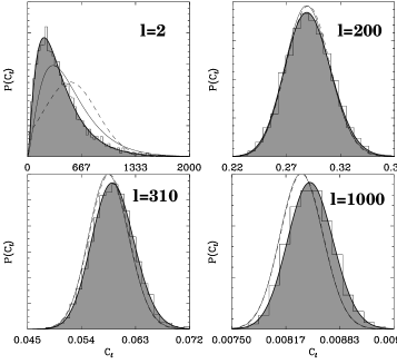
2. An exact analytical closed form solution for the non-Gaussian marginal probability distributions of the $\tilde{C}_{l}$. Examples of these distributions are shown in Figure 2.

   

   Figure 2: The $\tilde{C}_{l}$ distributions. We compute them for the standard cold dark matter model (shaded), the $\chi^{2}$ (solid lines) and the Gaussian (dashed) approximations compared to Monte Carlo simulations (histograms) for l=2,200,310,1000.

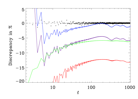
3. Exact expressions for cumulants and joint cumulants (and hence moments) of all orders for the $\tilde{C}_{l}$. In Figure 3 we compare the true means, standard deviation, skewness and kurtosis to the ones for the $\chi^{2}$ distribution for all $l$. These can form the basis of a debiasing scheme, as suggested in Wandelt Hivon & Górski (1998a).

   

   Figure 3: Moment discrepancies between the WHG and $\chi^{2}$ distributions. We show the discrepancy in percent between the means, standard deviations, skewness and kurtosis for the $\tilde{C}_{l}$ and $\chi^{2}$ distributions. The stars are the $\langle\tilde{C}_{l}\rangle$ computed from 3328 Monte Carlo simulations, showing excellent agreement only limited by Monte Carlo noise. Notice the oscillatory features in the discrepancy which indicate that it is dependent on the underlying theory, e.g. through the position and amplitude of the peaks. The difference in the means for $l\gtrsim 30$ is dominated by the correlation bias and does not decay for large $l$.

4. A new, standardised, $\chi^{2}$ distributed statistic $y_{l}$ which measures the goodness of fit between a set of observed $\tilde{C}_{l}$ and a given theory.

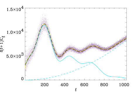
5. The discovery and removal of a correlation bias in cosmological parameter estimation which results from neglecting the correlations induced by partial sky coverage and anisotropic noise. This is an effect which is distinct from and in addition to the bias which comes from neglecting the non-Gaussianity of the $\tilde{C}_{l}$. This non-Gaussianity bias has been termed “cosmic” bias elsewhere (Bond, Jaffe, & Knox 1998b). The correlation bias occurs at all $l$ even those where the Central Limit Theorem ensures Gaussianity in the case of almost full sky coverage. . To show the effect on the estimation of cosmological parameters we form an approximate likelihood by multiplying the marginal $\tilde{C}_{l}$-distributions and use this to estimate $\Omega_{b}$, the baryon fraction for the standard cold dark matter scenario. The results are shown in Figure 4. While this is quite a small effect for the almost full sky case considered in Wandelt, Hivon & Górski (1998a) we conjecture this to become more important for medium to small sky coverage.

Figure 4: Correlation bias in cosmological parameter estimation. We estimate the baryon fraction in the universe from 17 realisations of $\tilde{C}_{l}$, comparing the Gaussian and $\chi^{2}$ approximation to our likelihood (WHG). The true value is marked with the long solid horizontal line. The mean estimates are marked with short horizontal lines. Because we enforce the correct marginal distributions our result is guaranteed to be unbiased while the Gaussian and $\chi^{2}$ approximations neglect $l$ to $l$ correlations and hence produce a systematic bias, here detected at more than 3 sigma (dashed horizontal lines).

The computation of any of these quantities, except for the joint moments, scales strictly as $N_{pix}^{3\over 2}$, where $N_{pix}$ is the number of pixels, with a small prefactor. This means all computation take on the order of 1 minute for an $l$-range of 0 to 1024. In the case of the joint moment $\left\langle\Delta\tilde{C}_{l}\Delta\tilde{C}_{l^{\prime}}\right\rangle$ the computation scales as $N_{pix}^{2}$ and takes on the order of a few minutes. Work is in progress to extend these methods to a viable tool for the joint estimation of the Big Bang $C_{l}$ and cosmological parameters in Gaussian theories from noisy, cut-sky data (Wandelt, Hivon & Górski 1998b).

References

- [1] Bersanelli M. et al., 1996, “COBRAS/SAMBA: Report on the Phase A Study”, see also http://astro.estex.esa.nl/Planck/
- [2] Bond J. R., Efstathiou G., Tegmark M., 1998, MNRAS, 291, L33
- [3] Bond J. R., Jaffe A., Knox L., 1998a, Phys. Rev. D, 57, 2117
- [4] Bond J. R., Jaffe A., Knox L., 1998b, Radical compression of cosmic microwave background data, astro-ph/9808264
- [5] Jungman G., Kamionkowski M., Kosowsky A., Spergel D. N., 1995, Phys. Rev. D, 54, 1332
- [6] Knox L., 1995, Phys. Rev. D, 52, 4307
- [7] Oh S. P., Spergel D. N., Hinshaw G., 1998, An efficient technique to determine the power spectrum from cosmic microwave backkground sky maps, astro-ph/9805339, Ap. J. in press
- [8] Tegmark M., 1997, Phys. Rev. D, 55, 5895
- [9] Wandelt B. D., Hivon E., Górski K., 1998a, Cosmic microwave background anisotropy power spectrum statistics for high precision cosmology, astro-ph/9808292
- [10] Wandelt B. D., Hivon E., Górski K. M., 1998b, in preparation
- [11] Zaldarriaga M., Spergel D., Seljak U., 1997, Ap. J., 488, 1