Gas Dynamics and Large–Scale Morphology of the Milky Way Galaxy

Abstract

We present a new model for the gas dynamics in the galactic disk inside the Sun’s orbit. Quasi–equilibrium flow solutions are determined in the gravitational potential of the deprojected COBE NIR bar and disk, complemented by a central cusp and, in some models, an outer halo. These models generically lead to four–armed spiral structure between corotation of the bar and the solar circle; their large–scale morphology is not sensitive to the precise value of the bar’s pattern speed, to the orientation of the bar with respect to the observer, and to whether or not the spiral arms carry mass.

Our best model provides a coherent interpretation of many observed gas dynamical features. Its four-armed spiral structure outside corotation reproduces quantitatively the directions to the five main spiral arm tangents at $|l|\leq 60^{\circ}$ observed in a variety of tracers. The 3-kpc-arm is identified with one of the model arms emanating from the ends of the bar, extending into the corotation region. The model features an inner gas disk with a cusped orbit shock transition to an $x_{2}$ orbit disk of radius $R\sim 150{\rm\,pc}$.

The bar’s corotation radius is fairly well–constrained at $R_{c}\simeq 3.5\pm 0.5{\rm\,kpc}$. The best value for the orientation angle of the bar is probably $20-25^{\circ}$, but the uncertainty is large since no detailed quantitative fit to all features in the observed ($l,v$) diagrams is yet possible. The Galactic terminal velocity curve from HI and CO observations out to $l\simeq\pm 45^{\circ}$ ($\sim 5{\rm\,kpc}$) is approximately described by a maximal disk model with constant mass–to–light ratio for the NIR bulge and disk.

1 Introduction

Although the Milky Way is in many ways the best studied example of a disk galaxy, it has proven exceedingly difficult to reliably determine its large–scale properties, such as the overall morphology, the structural parameters of the main components, the spiral arm pattern, and the shape of the Galactic rotation curve. A large part of this difficulty is due to distance ambiguities and to the unfortunate location of the solar system within the Galactic dust layer, which obscures the stellar components of the Galaxy in the optical wavebands. With the advent of comprehensive near–infrared observations by the COBE/DIRBE satellite and other ground- and space–based experiments, this situation has improved dramatically. These data offer a new route to mapping out the Galaxy’s stellar components, to connecting their gravitational potential with the available gas and stellar kinematic observations, and thereby to understanding the large–scale structure and dynamics of the Milky Way Galaxy.

From radio and mm–observations it has long been known that the atomic and molecular gas in the inner Galaxy does not move quietly on circular orbits: “forbidden” and non–circular motions in excess of $100{\rm\,km\,s^{-1}}$ are seen in longitude–velocity ($l,v$)–diagrams (e.g., Burton & Liszt 1978, Dame et al. 1987, Bally et al. 1987). Some of the more prominent features indicating non–circular motions are the $3{\rm\,kpc}$–arm, the molecular parallelogram (“expanding molecular ring”), and the unusually high central peak in the terminal velocity curve at $l\simeq\pm 2^{\circ}$. Many papers in the past have suggested that these forbidden velocities are best explained if one assumes that the gas moves on elliptical orbits in a barred gravitational potential (Peters 1975, Cohen & Few 1976, Liszt & Burton 1980, Gerhard & Vietri 1986, Mulder & Liem 1986, Binney et al. 1991, Wada et al. 1994).

In the past few years, independent evidence for a bar in the inner Galaxy has been mounting from NIR photometry (Blitz & Spergel 1991, Weiland et al. 1994, Dwek et al. 1995), from IRAS and clump giant source counts (Nakada et al. 1991, Whitelock & Catchpole 1992, Nikolaev & Weinberg 1997, Stanek et al. 1997), from the measured large microlensing optical depth towards the bulge (Paczynski et al. 1994, Zhao, Rich & Spergel 1996) and possibly also from stellar kinematics (Zhao, Spergel & Rich 1994). See Gerhard (1996) and Kuijken (1996) for recent reviews.

The currently best models for the distribution of old stars in the inner Galaxy are based on the NIR data from the DIRBE experiment on COBE. Because extinction is important towards the Galactic nuclear bulge even at $2\,\mu$m, the DIRBE data must first be corrected (or ‘cleaned’) for the effects of extinction. This has been done by Spergel, Malhotra & Blitz (1996), using a fully three-dimensional model of the dust distribution (see also Freudenreich 1998). Binney, Gerhard & Spergel (1997, hereafter BGS) used a Richardson–Lucy algorithm to fit a non-parametric model of $j({\bf r})$ to the cleaned data of Spergel et al. under the assumption of eight-fold (triaxial) symmetry with respect to three mutually orthogonal planes. When the orientation of the symmetry planes is fixed, the recovered emissivity $j({\bf r})$ appears to be essentialy unique (see also Binney & Gerhard 1996, Bissantz et al. 1997), but physical models matching the DIRBE data can be found for a range of bar orientation angles, $15^{\circ}\mathrel{\hbox to0.0pt{\lower 3.0pt\hbox{$\mathchar 536\relax$}\hss}\raise 2.0pt\hbox{$\mathchar 316\relax$}}\varphi_{\rm bar}\mathrel{\hbox to0.0pt{\lower 3.0pt\hbox{$\mathchar 536\relax$}\hss}\raise 2.0pt\hbox{$\mathchar 316\relax$}}35^{\circ}$ (BGS). $\varphi_{\rm bar}$ measures the angle in the Galactic plane between the bar’s major axis at $l>0$ and the Sun–centre line. For the favoured $\varphi_{\rm bar}=20^{\circ}$, the deprojected luminosity distribution shows an elongated bulge with axis ratios 10:6:4 and semi–major axis $\sim 2{\rm\,kpc}$, surrounded by an elliptical disk that extends to $\sim 3.5{\rm\,kpc}$ on the major axis and $\sim 2{\rm\,kpc}$ on the minor axis.

Outside the bar, the NIR luminosity distribution shows a maximum in the emissivity $\sim 3{\rm\,kpc}$ down the minor axis, which corresponds to the ring–like structure discussed by Kent, Dame & Fazio (1991), and which might well be due to incorrectly deprojected strong spiral arms. From the study of HII-Regions, molecular clouds and the Galactic magnetic field it appears that the Milky Way may have four main spiral arms (Georgelin & Georgelin 1976, Caswell & Heynes 1987; Sanders, Scoville & Solomon 1985, Grabelsky et al. 1988; Vallée 1995). These are located outside the $3{\rm\,kpc}$-arm in the ($l,v$) diagram and are probably related to the so–called molecular ring (Dame 1993), although it is unclear precisely how. One problem with this is that the distances to the tracers used to map out the spiral arms are usually computed on the basis of a circular gas flow model. The errors due to this assumption are not likely to be large, but cannot be reliably assessed until more realistic gas flow models including non–circular motions are available.

The goal of this paper is to construct gas-dynamical models for the inner Milky Way that connect the Galactic bar/bulge and disk as observed in the COBE NIR luminosity distribution with the kinematic observations of HI and molecular gas in the ($l,v$) diagram. In this way we hope to constrain parameters like the orientation, mass, and pattern speed of the bar, and to reach a qualitative understanding of the Galactic spiral arms and other main features in the observed ($l,v$) diagrams.

In barred potentials, gas far from resonances settles on periodic orbits such as those of the $x_{1}$- and $x_{2}$-orbit families, and some important aspects of the gas flow can be understood by considering the closed periodic orbits (e.g., Binney et al. 1991). However, near transitions of the gas between orbit families, along the leading edges of the bar, and in spiral arms, shocks form in the gas flow which can only be studied by gas dynamical simulations (e.g., Roberts, van Albada & Huntley 1979, Athanassoula 1992b, Englmaier & Gerhard 1997).

In this paper, we use the Smoothed Particle Hydrodynamics (SPH) method to study the gas flow in the gravitational potential of the non-parametrically deprojected COBE/DIRBE light distribution of Binney, Gerhard & Spergel (1997), assuming a constant mass to NIR luminosity ratio. The gas settles to an approximately quasi–stationary flow, and the resulting model ($l,v$) diagrams enable us to understand many aspects of the observations of HI and molecular gas.

The paper is organized as follows. In Section 2 we give a brief review of the main observational constraints, followed in Section 3 by a description of our models for the mass distribution and gravitational potential, and for the treatment of the gas. Section 4 describes the results from a sequence of gas dynamical models designed to constrain the most important parameters, and compares these models with observations. Our results and conclusions are summarized in Section 5.

2 Summary of observational constraints

2.1 Surveys and ($l,v$) diagrams

The kinematics and distribution of gas in the Milky Way disk have been mapped in 21-cm neutral hydrogen emission and in mm-line emission from molecular species, most notably ¹²CO. HI surveys include Burton (1985), Kerr et al. (1986), Stark et al. (1992) and Hartmann & Burton (1997), surveys in ¹²CO include Sanders et al. (1986), Dame et al. (1987) and Stark et al. (1988), and the most comprehensive survey in ¹³CO is that of Bally et al. (1987). The large scale morphology of the gas based on these data is discussed in the review by Burton (1992).

These surveys show a complicated distribution of gas in longitude–latitude–radial velocity $(l,b,v_{r})$ space or, integrating over some range in latitude, in the so–called ($l,v$) diagram. Fig. 1 shows an ($l,v$) diagram observed in ¹²CO by Dame et al. (1998, see also Dame et al. 1987) and transformed by them to the LSR frame by subtracting $|\mn@boldsymbol{v_{\odot}}|=20{\rm\,km\,s^{-1}}$ towards $(l,b)=(56.2^{\circ},22.8^{\circ})$ for the motion of the Sun with respect to the LSR (This corresponds to inward radial and forward components of the solar motion of $u_{\odot}=-10.3{\rm\,km\,s^{-1}}$ and $v_{\odot}=15.3{\rm\,km\,s^{-1}}$.) The general morphology of the ($l,v$) diagram in ¹²CO is broadly similar to that obtained from HI 21-cm emission (see, e.g., Burton 1992).

In general, no additional distance information for the gas is available; thus – unlike in the case of external galaxies – the spatial distribution of galactic gas cannot be directly inferred. Converting line–of–sight velocities to distances, on the other hand, requires a model of the gas flow.

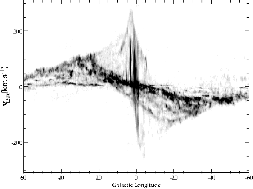
Figure 1: ($l,v$) diagram for ¹²CO from unpublished data by Dame et al. (1998). This figure contains all emission integrated over latitudes between $b=-2^{\circ}$ and $b=2^{\circ}$. The grey scale is adjusted such as to emphasize spiral arm structures.

2.2 Interpretation of ($l,v$) diagrams

For the comparison of observed and model ($l,v$) diagrams, it is useful to first consider an axisymmetric disk with gas in circular rotation (e.g., Mihalas & Binney 1981). In this model, an observer on a circular orbit will find the following results:

(i) Gas on the same circular orbit as the observer will have zero relative radial velocity.

(ii) For clouds on a different circular orbit with velocity $v(R)$, the measured radial velocity is

$$v_{r}=(\omega-\omega_{0})R_{0}\sin l,$$ (1)

where $\omega(R)\equiv v(R)/R$ is the angular rotation rate, $R_{0}$ is the galactocentric radius of the observer, and the index $0$ to a function or variable denotes its value at $R_{0}$. From this equation we see that, as long as $\omega(R)$ decreases outwards, the radial velocities have the same sign as $\sin l$ for gas inside the observer, and the opposite sign for gas on circular orbits outside the observer.

(iii) For clouds inside the observers orbit ($-90<l<90^{\circ}$), the maximal radial velocity along a given line–of–sight $l$ is $v_{r}={\rm sign}(l)v(R)-V_{0}\sin l$. This so–called terminal velocity is reached at the tangent point to the circular orbit with $R=R_{0}\sin l$. For $l>0$ ($l<0$) $v_{r}$ increases (decreases) from zero for clouds near the observer to the terminal velocity at a distance corresponding to the circular orbit with $R=R_{0}\sin l$; it then decreases (increases) again with distance from the observer and changes sign when crossing the observer’s radius at the far side of the Galaxy. The terminal velocities define the upper (lower) envelope in the ($l,v$) diagram for $0<l<90^{\circ}$ ($-90^{\circ}<l<0$).

(iv) A circular orbit of given radius follows a sinusoidal path in the ($l,v$) diagram[cf. equation (1)], within a longitude range bounded by $l=\pm\arcsin(R/R_{0})$. In the inner Galaxy ($-45^{\circ}\mathrel{\hbox to0.0pt{\lower 3.0pt\hbox{$\mathchar 536\relax$}\hss}\raise 2.0pt\hbox{$\mathchar 316\relax$}}l\mathrel{\hbox to0.0pt{\lower 3.0pt\hbox{$\mathchar 536\relax$}\hss}\raise 2.0pt\hbox{$\mathchar 316\relax$}}45^{\circ}$) circular orbits thus approximately trace out straight lines through the orgin in the ($l,v$) diagram.

(v) The edge of the Galaxy (the outermost circular orbit) results in a sine shaped envelope in the ($l,v$) diagram with negative radial velocities for positive longitudes ($0^{\circ}<l<180^{\circ}$) and vice versa. The sign of $v_{r}$ on this envelope is different from that on the terminal velocity envelope.

(vi) For a circular orbit model, one can derive the rotation curve of the inner Galaxy from the observed terminal velocities and eq. (1). This requires knowledge of the galactocentric radius $R_{0}$ and rotation velocity $V_{0}$ of the local standard of rest (LSR) as well as the motion of the Sun with respect to the LSR.

Fig. 1 and similar HI 21 cm ($l,v$) diagrams (see, e.g., Burton 1992) show gas between $90^{\circ}$ and $-90^{\circ}$ longitude whose radial velocities have the wrong sign for it to be gas on circular orbits inside the solar radius. Yet this gas is evidently connected to other gas in the inner Galaxy and is not associated with gas from outside the solar radius. These so–called forbidden velocities, up to $v_{r}\simeq 100{\rm\,km\,s^{-1}}$, are a direct signature of non–circular orbits in the inner Galaxy, and they have been the basis of previous interpretations of the inner Galaxy gas flow in terms of a rotating bar potential (e.g., Peters 1975, Mulder & Liem 1986, Binney et al. 1991).

One of the most prominent such features is the so–called $3{\rm\,kpc}$–arm, visible in Fig. 1 as the dense ridge of emission extending from $(l\simeq 10^{\circ},v=0)$ through $(l=0,v\simeq-50{\rm\,km\,s^{-1}})$ to $(l\simeq-22^{\circ},v\simeq-120{\rm\,km\,s^{-1}})$.

At longitudes $|l|\mathrel{\hbox to0.0pt{\lower 3.0pt\hbox{$\mathchar 536\relax$}\hss}\raise 2.0pt\hbox{$\mathchar 318\relax$}}25^{\circ}$, the circular orbit model is a reasonable description of the observed gas kinematics. Most of the emission in ¹²CO in fact comes from a gas annulus between about 4 and $7\,\rm kpc$ galactocentric radius, the so–called molecular ring (e.g., Dame 1993), which probably consists of two pairs of tightly wound spiral arms (see Section 4). A detailed interpretation of spiral arms in the ($l,v$) diagram requires a full gas dynamical model, as high intensities in Fig. 1 can be due to either high intrinsic gas densities or due to velocity crowding.

2.3 Terminal velocities

The top left and bottom right envelopes on the ($l,v$) diagram in Fig. 1 mark the terminal velocities. The terminal velocity curves will be used below for comparing with different models and for calibrating the models’ mass–to–light ratios. As will be seen in §4.4 below, the terminal velocities in ¹²CO and HI 21cm and between different surveys agree to a precision of $\sim 10{\rm\,km\,s^{-1}}$ in most places, but there are some regions with larger discrepancies.

Of particular interest is the strong peak in the terminal velocity curve with $v_{t}\simeq 260{\rm\,km\,s^{-1}}$ at $l\simeq 2^{\circ}$. Outwards from there the drop in $v_{t}$ is very rapid; for a constant mass–to–infrared luminosity ratio it would be nearly Keplerian and would be hard to reproduce in an axisymmetric bulge model (Kent 1992). Instead, the rapid drop is probably connected with a change of orbit shape over this region (Gerhard & Vietri 1986). In the model of Binney et al. (1991), the peak is associated with the cusped orbit in the rotating barred potential, and the subsequent drop of $v_{t}$ with $l$ reflects the shapes of the adjacent $x_{1}$–orbits.

2.4 Spiral arms

From distant galaxies we know that spiral arms are traced by molecular gas emission. Indeed one can identify some of the dense emission ridges in Fig. 1 with Galactic spiral arms; where these meet the terminal velocity curve, they can be recognized as ‘bumps’ where $\partial v_{t}/\partial l\simeq 0$. In addition, spiral arms are clearly visible in the distribution of various tracers, such as HII regions.

Fig. 2 shows an ($l,v$) diagram of several classes of objects which are useful as discrete tracers of dense gas in spiral arms. On each side, we can identify two spiral arm tangents at around $\pm\sim 30$ and $\pm\sim 50^{\circ}$. On the northern side, the $\sim 30^{\circ}$ component splits up into two components at $\sim 30^{\circ}$ and $\sim 25^{\circ}$ longitude, which is also evident from the Solomon et al. (1985) data.

Table 1 lists a number of tracers that have been used to delineate spiral arms. The inferred spiral arm tangents coincide with features along the terminal curve in Fig. 1; compare also Fig. 1 and Fig. 2. In the inner Galaxy there are thus five main arm tangents, of which the Scutum tangent is double in a number of tracers. The inner Scutum tangent at $l\simeq 25^{\circ}$ is sometimes referred to as the northern 3–kpc arm.

While the main spiral arm tangents on both sides of the Galactic center are thus fairly well–determined, it is much less certain how to connect the tangents on both sides. From the distribution of HII-Regions, Georgelin & Georgelin (1976) sketched a four spiral arm pattern ranging from about $4\,\rm kpc$ galactocentric radius to beyond the solar radius. Although their original pattern has been slightly modified by later work, the principal result of a four–armed spiral structure has mostly been endorsed (see the review in Vallée 1995).

For illustration, Fig. 2 also shows the traces in the ($l,v$) diagram of the spiral arms in our standard no–halo model (see Section 4). This model has two pairs of arms emanating from the end of the COBE bar, and a four–armed spiral pattern outside the bar’s corotation radius. The model matches the observed tangents rather well and illustrates the ways in which they can be connected.

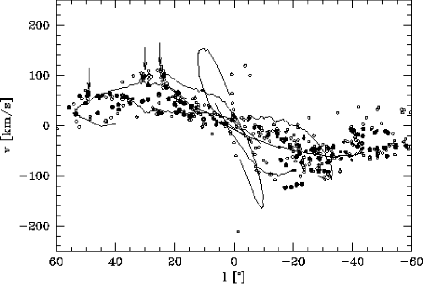
Figure 2: ($l,v$) diagram for HII regions from Georgelin & Georgelin (1976), Downes et al. (1980) and Caswell & Haynes (1987) (open circles); and for massive molecular clouds from Dame et al. (1986) and Bronfman (1989) (filled circles). The arrows point to the positions of the densest clusters of warm CO clouds along the terminal curve, which are presumably located in spiral arm shocks (Solomon, Sanders & Rivolo 1985). For the sake of clarity, clouds with less than $10^{5.5}\,M_{\odot}$ have been omitted from Bronfman’s data, as well as clouds within the smallest brightness bin from the Georgelin & Georgelin sample. For illustration, the thin lines show the locations of the gas spiral arms in our standard $\varphi_{\rm bar}=20^{\circ}$ COBE bulge and disk model without dark halo; cf. Section 4.

Inner Galaxy spiral arm tangents in longitude					Measurement	Ref.
Scutum	Sagittarius	Centaurus	Norma	3-kpc
29	50	-50	-32		HI	Weaver (1970), Burton & Shane (1970), Henderson (1977)
24, 30.5	49.5	-50	-30		integrated 12CO	Cohen et al.  (1980), Grabelsky et al.  (1987)
25, 32	51				12CO clouds	Dame et al.  (1986)
25, 30	49				warm CO clouds	Solomon et al.  (1985)
24, 30	47	-55	-28		HII-Regions (H109-$\alpha$)	Lockman (1979), Downes et al.  (1980)
32	46	-50	-35		26Al	Chen et al.  (1996)
32	48	-50,-58	-32	-21	Radio $408\,\,{\rm MHz}$	Beuermann et al.  (1985)
29			-28	-21	$2.4\,{\mu\rm m}$	Hayakawa et al.  (1981)
26		-47	-31	-20	$60\,{\mu\rm m}$	Bloemen et al.  (1990)
30	49	-51	-31	-21	adopted mean
$\sim 25$	54	-44	-33	-20	$R_{c}=3.4{\rm\,kpc}$, $\varphi_{\rm bar}=20^{\circ}$, without halo
$\sim 30$	50	-46	-33	-20	$R_{c}=3.4{\rm\,kpc}$, $\varphi_{\rm bar}=20^{\circ}$, with halo $v_{0}=200{\rm\,km\,s^{-1}}$
$\sim 29$	51	-47	-34	-22	$R_{c}=3.4{\rm\,kpc}$, $\varphi_{\rm bar}=25^{\circ}$, with halo $v_{0}=200{\rm\,km\,s^{-1}}$

Table 1: Observed spiral arm tangents compared to model predictions.

2.5 Dense gas in the Galactic Centre

Dense regions, where the interstellar medium becomes optically thick for 21-cm line or ¹²CO emission, can still be observed using rotational transition lines of ¹³CO, CS, and other rare species. In the ¹³CO emission line, which probes regions with $\sim 40$ times higher volume densities than the ¹²CO line, an asymmetric parallelogram–like structure between $\sim+1.5^{\circ}$ and $\sim-1^{\circ}$ in longitude is visible (Bally et al. 1988). This is nearly coincident with the peak in the terminal velocity curve and has been associated with the cusped $x_{1}$-orbit by Binney et al. (1991); see also Section 4. In this interpretation, part of the asymmetry is accounted for by the perspective effects expected for this elongated orbit with a bar orientation angle $\varphi_{\rm bar}=20^{\circ}$.

At yet higher densities, the CS line traces massive molecular cloud complexes, which are presumably orbiting on $x_{2}$-orbits inside the bar’s Inner Lindblad Resonance (Stark et al. 1991, Binney et al. 1991). These clouds appear to have orbital velocities of $\mathrel{\hbox to0.0pt{\lower 3.0pt\hbox{$\mathchar 536\relax$}\hss}\raise 2.0pt\hbox{$\mathchar 316\relax$}}100{\rm\,km\,s^{-1}}$.

2.6 Tilt and asymmetry

We should finally mention two observational facts that are not addressed in this paper. Firstly, the gaseous disk between the $x_{2}$-disk and the 3-kpc-arm is probably tilted out of the Galactic plane. Burton & Liszt (1992) give a tilt angle of about $13^{\circ}$ for the HI distribution and show that, by combining this with the effects of a varying vertical scale height, the observed asymmetry in this region can be explained. Heiligman (1987) finds a smaller tilt of $\sim 7^{\circ}$ for the parallelogram.

Secondly, the molecular gas disk in the Galactic Center is highly asymmetric. Three quarters of the ¹³CO and CS emission comes from positive longitudes and a different three quarters comes from material at positive velocities (Bally et al. 1988). Part of the longitude asymmetry may be explained as a perspective effect, and part of both asymmetries is caused by the one–sided distribution of the small number of giant cloud complexes. Nonetheless it is possible that the observed asymmetries signify genuine deviations from a triaxially symmetric potential.

2.7 Solar radius and velocity – comparing real and model ($l,v$) diagrams

A model calculation results in a velocity field as a function of position, with the length–scale set by the distance to the Galactic Center assumed in the deprojection of the COBE bulge (Binney, Gerhard & Spergel 1997). These authors took $R_{0}=8{\rm\,kpc}$, and throughout this paper we will use this value in comparing our models to observations. To convert model velocity fields into ($l,v$) diagrams as viewed from the LSR, we scale by a constant factor (this gives the inferred mass–to–light ratio) and then subtract the line–of–sight component of the tangential velocity of the LSR, assuming $V_{0}=200{\rm\,km\,s^{-1}}$. This value is in the middle of the range consistent with various observational data (Sackett 1997), and is also a reasonable value to use if the Galactic potential near the Sun is slightly elliptical (Kuijken & Tremaine 1994). If the model has a constant circular rotation curve, i.e., if it includes a dark halo, the LSR velocity is part of the model and is scaled together with the gas velocities. For these models the final scaled LSR tangential velocity will be different from $V_{0}=200{\rm\,km\,s^{-1}}$ and will be stated in the text. The radial velocity of the LSR has been set to zero throughout this paper.

3 The models

In this Section, we describe in more detail the models that we use to study the gas flow in the gravitational potential of the Galactic disk and bulge, as inferred from the COBE/DIRBE NIR luminosity distribution. In some of these models the gravitational field of a dark halo component is added. Self–gravity of the gas and spiral arms are not taken into account until §4.7. In the following, we first describe our mass model as derived from the COBE/DIRBE NIR data (§3.1), then the resulting gravitational potential (§3.2) and closed orbit structure (§3.3), the assumptions going into the hydrodynamical model (§3.4), and finally the main free parameters in the model (§3.5).

3.1 Mass model from COBE NIR luminosity distribution

The mass distribution in the model is chosen to represent the luminous mass distribution as closely as possible. From the NIR surface brightness distribution as observed by the COBE/DIRBE experiment, Spergel et al. (1996) computed dust–corrected NIR maps of the bulge region using a three–dimensional dust model. These cleaned maps were deprojected by the non–parametric Lucy–Richardson algorithm of Binney & Gerhard (1996) as described in Binney, Gerhard & Spergel (1997; BGS). The resulting three–dimensional NIR luminosity distributions form the basis of the mass models used in this paper.

The basic assumption that makes the deprojection of BGS work is that of eight–fold triaxial symmetry, i.e., the luminosity distribution is assumed to be symmetric with respect to three mutually orthogonal planes. For general orientation of these planes, a barred bulge will project to a surface brightness distribution with a noticeable asymmetry signal, due to the perspective effects for an observer at $8{\rm\,kpc}$ distance from the Galactic Center (Blitz & Spergel 1991). Vice–versa, if the orientation of the three symmetry planes is fixed, the asymmetry signal in the data can be used to infer the underlying triaxial density distribution (Binney & Gerhard 1996). Because of the assumed symmetry, neither spiral structure nor lopsidedness can be recovered by the eight–fold algorithm. However, spiral arm features in the NIR luminosity may be visible in the residual maps, and may appear as symmetrized features in the recovered density maps.

The orientation of the three orthogonal planes is specified by two angles. One of these specifies the position of the Sun relative to the principal plane of the bulge/bar; this angle takes a well–determined (small) value such that the Sun is approximately $14{\rm\,pc}$ above the equatorial plane of the inner Galaxy (BGS). The other angle $\varphi_{\rm bar}$ specifies the orientation of the bar major axis in the equatorial plane relative to the Sun–Galactic Center line; this angle is not well–determined by the projected surface brightness distribution. However, for a fixed value of the assumed $\varphi_{\rm bar}$, an essentially unique model for the recovered 3D luminosity distribution results: BGS demonstrated that their deprojection method converges to essentially the same solution for different initial luminosity distributions used to start the iterations (see also Bissantz et al. 1997). As judged from the surface brightness residuals, the residual asymmetry map, and the constraint that the bar axial ratio should be $<1$, admissable values for the bar inclination angle $\varphi_{\rm bar}$ are in the range of $15^{\circ}$ to $35^{\circ}$. We will thus investigate gas flow models with $\varphi_{\rm bar}$ in this range.

For the favoured (BGS) $\varphi_{\rm bar}=20^{\circ}$, the deprojected luminosity distribution shows an elongated bulge/bar with axis ratios 10:6:4 and semi–major axis $\sim 2{\rm\,kpc}$, surrounded by an elliptical disk that extends to $\sim 3.5{\rm\,kpc}$ on the major axis and $\sim 2{\rm\,kpc}$ on the minor axis. Outside the bar, the deprojected NIR luminosity distribution shows a maximum in the emissivity $\sim 3{\rm\,kpc}$ down the minor axis, which appears to correspond to the ring–like structure discussed by Kent, Dame & Fazio (1991). The nature of this feature is not well understood. Possible contributions might come from stars on orbits around the Lagrange points (this appears unlikely in view of the results of §3.3 and §4.1 below), or from stars on $x_{1}$-orbits outside corotation or on the diamond shaped $1:4$ resonant orbits discussed by Athanassoula (1992a) (however, the feature is very strong). The most likely interpretation in our view, based on §4 below, is that this feature is due to incorrectly deprojected (symmetrized) strong spiral arms. If this interpretation is correct, then by including these features in our mass model we automatically have a first approximation for the contribution of the Galactic spiral arms to the gravitational field of the Galaxy.

In the following, we will model the distribution of luminous mass in the inner Galaxy by using the deprojected DIRBE L–band luminosity distributions for $15^{\circ}<\varphi_{\rm bar}<35^{\circ}$ and assuming a constant L–band mass–to–light ratio $M/L_{L}$. The assumption of constant $M/L_{L}$ may not be entirely correct if supergiant stars contribute to the NIR luminosity in star forming regions in the disk (Rhoads 1998); this issue will be investigated and discussed further in §4.1. To obtain a mass model for the entire Galaxy, we must extend the luminous mass distribution of BGS, by adding a central cusp and a model for the outer disk, and (in some cases) add a dark halo to the resulting gravitational potential.

3.1.1 Cusp

The density distribution of stars near the Galactic Center can be modelled as a power law $r^{-p}$. From star counts in the K–band the exponent $p\simeq 2.2\pm 0.2$ for K=6-8 mag stars (Catchpole, Whitelock & Glass 1990). The distribution of OH/IR stars near the center gives $p\simeq 2.0\pm 0.2$ (Lindqvist, Habing & Winnberg 1992). Using radial velocities of the OH/IR stars and the assumption of isotropy, Lindqvist et al. determined the mass distribution inside $\sim 100{\rm\,pc}$. The corresponding mass density profile has $p\simeq 1.5$ between $\sim 20{\rm\,pc}$ and $\sim 100{\rm\,pc}$ and steepens inside $\sim 20{\rm\,pc}$. The overall slope is approximately that originally found by Becklin & Neugebauer (1968, $p\simeq 1.8$).

In the density model obtained from the DIRBE NIR data, this central cusp is not recovered because of the limited resolution and grid spacing ($1.5^{\circ}$) in the dust corrected maps of Spergel et al. (1996). The cusp slope of the deprojected model just outside $1.5^{\circ}$ moreover depends on that in the initial model used to start the Lucy algorithm. To ensure that our final density model includes a central cusp similar to the observed one, we have therefore adopted the following procedure. For the initial model used in the deprojection, we have chosen a cusp slope of $p=1.8$, in the middle of the range found from star counts and mass modelling. This gives a power law slope of $p=1.75$ in the final deprojected density model at around $400{\rm\,pc}$. We have then expanded the deprojected density in multipoles $\rho_{lm}(r)$ and have fitted power laws to all $\rho_{l0}$ in the radial range $350-500{\rm\,pc}$. Inside $350{\rm\,pc}$ these density multipoles were then replaced by the fitted power laws, extrapolating the density inwards. The $m\not=0$ terms were not changed; they decay to zero at the origin. By this modification the mass inside $350{\rm\,pc}$ is approximately doubled. The implied change in mass is small compared to the total mass of the bulge and is absorbed in a slightly different mass-to-light ratio when scaling the model to the observed terminal velocity curve.

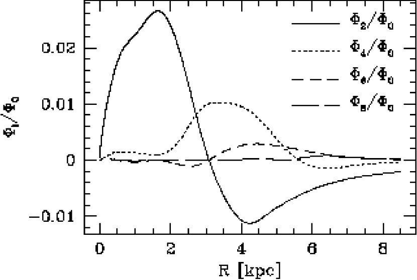
Figure 3: Contribution of various planar multipoles to the potential of the standard $\varphi_{\rm bar}=20^{\circ}$ bar model.

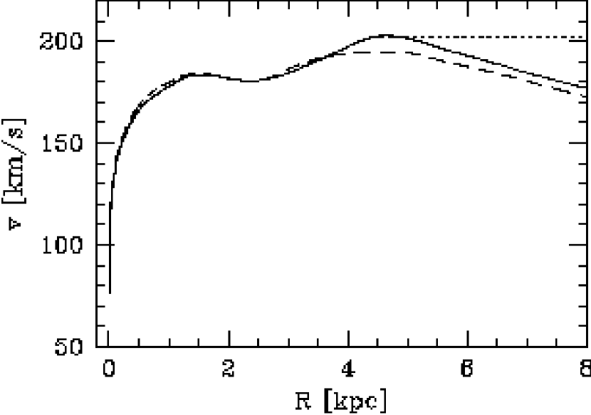
Figure 4: Rotation curve in the standard $\varphi_{\rm bar}=20^{\circ}$ model (solid line), in the model with substracted ring (dashed), and a model with constant outer rotation curve (dotted). The rotation curves are given for a scaling constant of $\xi=1.075$.

3.1.2 Outer disk

The deprojected luminosity model of BGS gives the density in the range $0<x,y<5\,\rm kpc$ and $0<z<1.4\,\rm kpc$. We thus need to use a parametric model for the mass density of the Galactic disk outside $R=5{\rm\,kpc}$. In this region the NIR emission is approximated by the analytic double–exponential disk model given by BGS. The least–squares fit parameters are $R_{d}=2.5{\rm\,kpc}$ for the radial scale–length, and $z_{0}=210{\rm\,pc}$ and $z_{1}=42{\rm\,pc}$ for the two vertical scale–heights. These parameters are very similar to those obtained by Kent, Dame & Fazio (1991) from their SPACELAB data. To convert this model for the outer disk luminosity into a mass distribution, we have assumed that the disk has the same $M/L_{L}$ as the bulge, because we cannot distinguish between the bulge and disk contributions to the NIR emission in the deprojected model for the inner Galaxy.

3.2 Gravitational potential

From the density model, we can compute the expansion of the potential in multipole components $\Phi_{lm}(r)$ and hence the decomposition

$$\Phi(r,\varphi)=\Phi_{0}(r)+\Phi_{2}(r,\varphi)\cos(2\varphi)+\Phi_{4}(r,\varphi)\cos(4\varphi)$$ (2)

in monopole $\Phi_{0}$, quadrupole $\Phi_{2}$, and octupole $\Phi_{4}$ terms. Higher order terms do not contribute enough to the forces to change the gas flow significantly (see Fig. 3), and are therefore neglected in the following. The advantage of this multipole approximation is that it is economical in terms of computer time (no numerical derivatives are needed for the force calculations). The quality of the expansion for the forces was tested with an FFT solver. Errors due to the truncation of the series are typically below $5{\rm\,km\,s^{-1}}$ in velocity. Because this is less than the sound speed, such errors will not significantly affect the gas flow.

As already mentioned, it is necessary to modify the potential near the center because of the unresolved central cusp in the COBE density distribution. As described above, we have replaced the multipole components of the density by power law fits inwards of $r=350{\rm\,pc}$ before computing the corresponding multipole expansion of the potential. Since the higher order multipoles $\rho_{l0}$ have smaller power law exponents than the $\rho_{00}$ term, this implies that the cusp becomes gradually spherically symmetric at small radii. We have chosen this approach because it did not require a specification of the shape of the central cusp. Note that without including the modified cusp the gravitational potential would not possess $x_{2}$ orbits and therefore the resulting gas flow pattern would be different. Fig. 3 shows the contribution of the various multipoles to the final COBE potential of our standard model with $\varphi=20^{\circ}$. The rotation curve obtained from this potential is shown in Fig 4.

3.2.1 Dark halo

If the Galactic disk and bulge are maximal, i.e., if they have the maximal mass–to–light ratio compatible with the terminal velocities measured in the inner Galaxy, then we do not require a significant dark halo component in the bar region. This may be close to the true situation because even with this maximal $M/L_{L}$ the mass in the disk and bulge fail to explain the high optical depth in the bulge microlensing data (Udalski et al. 1994, Alcock et al. 1997) by a factor $\mathrel{\hbox to0.0pt{\lower 3.0pt\hbox{$\mathchar 536\relax$}\hss}\raise 2.0pt\hbox{$\mathchar 318\relax$}}2$ (Bissantz et al. 1997). Thus in our modelling of the bar properties we have not included a dark halo component.

However, for the spiral arms found outside corotation of the bar, the dark halo is likely to have some effect. Since we only study the gas flow in the galactic plane, the force from the dark halo is easy to include without reference to its detailed density distribution. We simply change the monopole moment in the potential directly such that the asymptotic rotation curve becomes flat with a specified circular velocity. The rotation curve for our flat rotation model is also shown in Fig 4. In this model, the halo contribution to the radial force at the solar circle is $\simeq 23\%$.

3.3 Effective potential, orbits, and resonance diagram

 

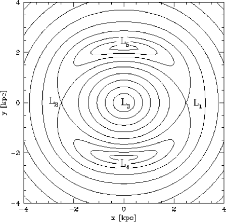
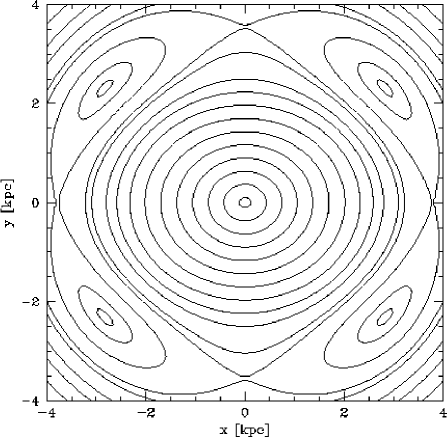
Figure 5: Left: Effective potential in the standard $\varphi_{\rm bar}=20^{\circ}$ bar model for $\Omega_{\rm P}=80\,\rm km\rm s^{-1}\rm kpc^{-1}$, showing the usual four Lagrangian points in the corotation region. Right: For $\Omega_{\rm P}=55\,\rm km\rm s^{-1}\rm kpc^{-1}$. Because the mass peaks in the disk $\sim 3{\rm\,kpc}$ down the bar’s minor axis now contribute significantly to the potential near the increased corotation radius, there are eight Lagrangian points near corotation for this pattern speed.

 

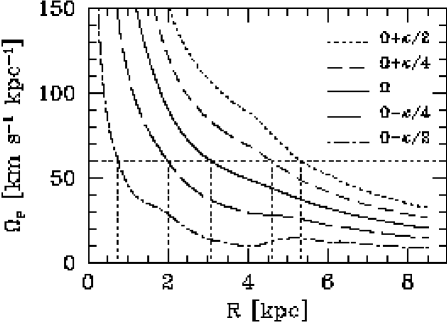
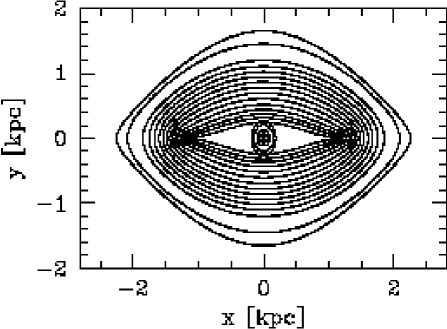
Figure 6: Left: Resonance diagram for the standard $\varphi_{\rm bar}=20^{\circ}$ bar model. Right: Some $x_{1}$ and $x_{2}$ orbits in this model for a pattern speed of $60\,\rm km\rm s^{-1}\rm kpc^{-1}$. The gap between the second and third orbit from outside shows the location of the $1:4$ resonance.

The constructed galaxy models have some special properties, due to the mass peaks in the disk $\sim 3{\rm\,kpc}$ down the minor axis of the bar. In the more common barred galaxy models, the effective potential

$$\Phi_{\rm eff}=\Phi-{1\over 2}\Omega_{P}^{2}R^{2}$$ (3)

in the rotating bar frame contains the usual four Lagrange points around corotation and a fifth Lagrange point in the centre. In our case, this is true only for larger pattern speeds $\Omega_{P}$, say $80\,\rm km\rm s^{-1}\rm kpc^{-1}$, when the corotation region does not overlap with the region affected by these (presumably) spiral arm features. For lower pattern speeds, in particular for $\Omega_{P}\simeq 55-60\,\rm km\rm s^{-1}\rm kpc^{-1}$ which we will find below to be appropriate for the Milky Way bar, the situation is different: in this case we obtain four stable and four unstable Lagrange points around corotation. The four unstable points lie along the principal axes where normally the four usual Lagrange points are located, whereas the stable Lagrange points lie between these away from the axes (see Fig. 5). For yet lower pattern speeds, the number of Lagrange points reduces to four again, but then the two usual saddle points have changed into maxima and vice versa.

We have not studied the orbital structure in this potential in great detail. However, some of the orbits we have found are shown in Fig. 6, demonstrating the existence of $x_{1}$, $x_{2}$, and resonant 1:4 orbits also in this case when there are eight Lagrange points near corotation. This is presumably due to the fact that these orbits do not probe the potential near corotation. For the orbit nomenclature used here see Contopoulos & Papayannopoulos (1980).

With appropriate scaling, the envelope of the $x_{1}$ orbits in our model follows the observed terminal curve in the longitude–velocity diagram, and the peak in the curve corresponds approximately to the cusped $x_{1}$ orbit, as in the model of Binney et al. (1991). This will be discussed further in §4.

3.4 Hydrodynamical Models

For the hydrodynamical models we have used the two–dimensional smoothed particles hydrodynamics (SPH) code described in Englmaier & Gerhard (1997). The gas flow is followed in the gravitational potential of the model galaxy as given by the multipole expansion described in §3.2, in a frame rotating with a fixed pattern speed $\Omega_{\rm P}$. In some later simulations we have included the self-gravity of the spiral arms represented by the gas flow (see §4.7 below).

All models assume point symmetry with respect to the centre. This effectively doubles the number of particles and leads to a factor of $\sqrt{2}$ improvement in linear resolution. We have checked that models without this symmetry give the same results, as would be expected because the background potential dominates the dynamics.

The hydrodynamic code solves Euler’s equation for an isothermal gas with an effective sound speed $c_{s}$:

$${\partial{\mathbf{v}}\over\partial t}+({\mathbf{v}}\cdot\nabla){\mathbf{v}}=-c_{\rm s}^{2}{\nabla\rho\over\rho}-\nabla\Phi.$$ (4)

This is based on the results of Cowie (1980) who showed that a crude approximation to the ISM dynamics is given by an isothermal single fluid description in which, however, the isothermal sound speed is not the thermal sound speed, but an effective sound speed representing the rms random velocity of the cloud ensemble.

Using the SPH method to solve Eulers equation has the advantage to allow for a spatially adaptive resolution length. The smoothing length $h$, which can be thought of denoting the particle size, is adjusted by demanding an approximately constant number of particles overlapping a given particle. The SPH scheme approximates the fluid quantities by averaging over neighboring particles and, in order to resolve shocks, includes an artificial viscosity. This can be understood as an additional viscous pressure term which allows the pre-shock region to communicate with the post-shock region, i.e., to transfer momentum. We have used the standard SPH viscosity (Monaghan & Gingold 1983) with standard parameters $\alpha=1$ and $\beta=2$. This SPH method was tested for barred galaxy applications by verifying that the properties of shocks forming in such models agree with those found by Athanassoula (1992b) with a grid-based method. See Steinmetz & Müller (1993) and Englmaier & Gerhard (1997) for further details.

In the low resolution calculations described below we have generally used 20000 SPH particles and have taken a constant initial surface density inside $7{\rm\,kpc}$ galactocentric radius. With the assumptions that the gas flow is two–dimensional and point–symmetric, these parameters give an initial particle separation in the Galactic plane of $62{\rm\,pc}$. High resolution calculations include up to 100,000 SPH particles and may cover a larger range in galactocentric radius to investigate the effects of the outer boundary.

We have experimented with two methods for the initial setup of the gas distribution. Method A starts the gas on circular orbits in the axisymmetric part $\Phi_{0}$ of the potential. Then the non-axisymmetric part of $\Phi$ is gradually introduced within typically one half rotation of the bar. Method B places the gas on $x_{1}$-orbits outside and on $x_{2}$-orbits inside the cusped $x_{1}$-orbit. The latter method leads to a more quiet start than the former, since the gas configuration is already closer to the final equilibrium. Most models shown in this paper have been set up with Method A. One model was created with a combination of both methods to improve resolution around the cusped orbit (see § 4.4).

Different models are usually compared at an evolutionary age of $0.3{\rm\,Gyr}$, when the gas flow has become approximately quasi-stationary (see §4.2). This corresponds to just under three particle rotation periods at a radius of $3{\rm\,kpc}$. The turn-on time of the bar is $\sim 0.04{\rm\,Gyr}$ and is included in the quoted evolution age.

Since the mass–to–light ratio of the model is not known a priori, all velocities in the model are known only up to a uniform scaling constant $\xi$. This implies that also the final sound speed is scaled from the value used in the numerical calculation: If we know the solution $\mathbf{v}(\mathbf{r})$ in one potential $\Phi$ with galaxy mass $M$, and sound speed $c_{\rm s}$, then we also know the scaled solution $\xi\mathbf{v}(\mathbf{r})$ for the potential $\xi^{2}\Phi$, galaxy mass $\xi^{2}M$, and sound speed $\xi c_{\rm s}$. For the gas we thus effectively assume an isothermal equation of state with sound speed $c_{\rm s}=\xi\,10\,\rm km\rm s^{-1}$. Note that, because $c_{\rm s}$ is a local physical quantity, our model can not simply be scaled down to a dwarf size galaxy, because then the resulting sound speed would be too small and this matters because the gas flow pattern depends on this parameter (Englmaier & Gerhard 1997).

Below, we fix the scaling constant $\xi$ by fitting the terminal velocity curve of the model to the observed terminal velocity curve. To do this, we have to simultaneously assume a value for the local standard of rest (LSR) circular motion. These two parameters compensate to some extent, but we generally find that the fit to the terminal curve is more sensitive to the assumed LSR motion than to the value of the scaling constant. In most of the rest of the paper we have therefore fixed the LSR velocity to $200{\rm\,km\,s^{-1}}$. We work in units of ${\rm\,kpc}$, ${\rm\,Gyr}$, and $M_{\odot}$. If the deprojected COBE density distribution is assumed to be in units of $3\,10^{8}M_{\odot}{\rm\,kpc}^{-3}$, $\xi$ is found to have typical values of 1.075 to 1.12.

3.5 Summary of model parameters and discussion of assumptions

Our models have a small number of free parameters; these and the subset which are varied in this paper are listed here. This Section also contains a brief summary and discussion of the main assumptions.

3.5.1 Bar parameters

$\bullet$ Probably the most important parameter is the bar’s corotation radius $R_{c}$ or pattern speed $\Omega_{\rm P}$, which will set the location of the resonance radii and spiral arms and shocks in the gas flow.

$\bullet$ The second important bar parameter is its orientation angle $\varphi$ with respect to the Sun–Galactic Center line, which affects the appearance of the gas flow as viewed from the Sun.

The shape and radial density distribution in the bar region are constrained by the observed NIR light distribution. However, their detailed form is dependent on the assumption of 8-fold symmetry, which is likely to be a good assumption in the central bulge region, but might be too strong in the outer bar regions, where a possible spiral density wave might affect the dynamics. It is also possible that an overall $m=1$ perturbation is needed to explain the observed asymmetries, such as in the distribution of giant cloud complexes in the Galactic center, or the fact that the 3-kpc-arm appears to be much stronger than its counterarm. Nevertheless, it is important to find out how far we can go without these asymmetries. In any case, the bar should have the strongest impact on the dynamics.

3.5.2 Mass model

$\bullet$ The only additional parameter in the luminous mass model is the scaling constant $\xi$ which relates NIR luminosity and mass. For each pair of values of the previous two parameters and at fixed LSR rotation velocity this is determined from the Galactic terminal velocity curve, assuming that this is dominated by the luminous mass in the central few ${\rm\,kpc}$.

This contains the additional assumption that all components have the same constant NIR mass-to-light ratio. This appears to be a reasonably good assumption on the basis of the fact that optical–NIR colours of bulges and disks in external galaxies are very similar (Peletier & Balcells 1996). It is unlikely to be strictly correct, however, because the bulge and disk stars will not all have formed at the same time. To relax this assumption requires additional assumptions about the distinction between disk and bulge stellar luminosity. This is presently impractical.

$\bullet$ Depending on the LSR rotational velocity, a dark halo is required beyond $R\simeq 5{\rm\,kpc}$. Thus we need to specify the asymptotic circular velocity of the halo. Here we consider only two cases, one without halo, the other with asymptotic halo velocity of $v_{0}=200{\rm\,km\,s^{-1}}$. This is in the middle of the observed range of $180-220{\rm\,km\,s^{-1}}$ (Sackett 1997).

3.5.3 LSR motion and position

$\bullet$ We assume throughout this paper that the distance of the LSR to the galactic centre is $R_{0}=8\,\rm kpc$ (see the review by Sackett 1997, but also the recent study by Olling & Merrifield 1998, who argue for a somewhat smaller $R_{0}$).

To compare model velocity fields with observations, we have to know not only the position of the Sun but also its motion. The peculiar motion of the Sun relative to the LSR is often already corrected for in the published data.

$\bullet$ The remaining free parameter is the LSR rotational velocity around the galactic center, which lies in the range between $180-220{\rm\,km\,s^{-1}}$ (Sackett 1997). We will again use $V_{0}=200\,\rm km\rm s^{-1}$, consistent with the above.

3.5.4 Gas model

We use a crude approximation to the ISM dynamics, that of an isothermal single fluid (Cowie 1980). The effective sound speed $c_{s}$ is the cloud–cloud velocity dispersion; this varies from $\sim 6{\rm\,km\,s^{-1}}$ in the solar neighbourhood to $\sim 25{\rm\,km\,s^{-1}}$ in the Galactic Center gas disk. We have considered models with globally constant value of $c_{s}$ between $5-30{\rm\,km\,s^{-1}}$ and have not found any interesting effects. Only at the largest values do the spiral arm shocks become very weak.

Consistent with the assumption of eight–fold symmetry for the mass distribution, we have assumed the gas flow to be point symmetric with respect to the origin. For gas flows in the eight–fold symmetric potential and without self-gravity there are no significant differences to the case when the gas model is run without symmetry constraint.

4 Results

4.1 Gas flow morphology implied by the COBE luminosity/mass distribution

We begin by describing the morphology of gas flows in the COBE–constrained potentials. For our starting model we take the deprojected eight–fold symmetric luminosity distribution obtained from the cleaned COBE L-band data, for a bar angle $\varphi_{\rm bar}=20^{\circ}$ as favoured by BGS. This model, with constant mass–to–light ratio and no additional dark halo, will be referred to as the (standard) $\varphi_{\rm bar}=20^{\circ}$ COBE bar.

In our first simulation this bar model is assumed to rotate at a constant pattern speed $\Omega_{p}$ such that corotation is at a galactocentric radius of approximately $3.1{\rm\,kpc}$. With the value for the mass–to–light ratio $\Upsilon_{L}$ as determined by Bissantz et al. (1997) from fitting the observed terminal velocities, this gives $\Omega_{p}=60{\rm\,km\,s^{-1}}/{\rm\,kpc}$.

For the gas model we take a constant initial surface density on circular orbits, represented by 20000 SPH particles, and an effective isothermal sound speed of $c_{s}=10{\rm\,km\,s^{-1}}$. The gas is relaxed in the bar potential as described in §3.4 (Method A) and the initial particle separation in the Galactic plane is $62{\rm\,pc}$.

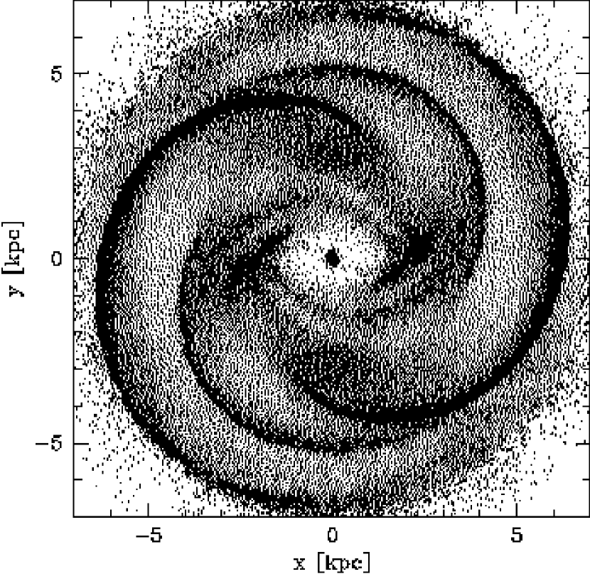
Figure 7: Gas flow in the $\varphi_{\rm bar}=20^{\circ}$ COBE bar with corotation at $R_{c}\simeq 3.1{\rm\,kpc}$. In this and subsequent figures, the long axis of the bar lies along the $x$-axis, and the location of the Sun is at $x=-7.5{\rm\,kpc}$, $y=-2.7{\rm\,kpc}$, $20^{\circ}$ away from the bar’s major axis. The simulation has $N=20000$ SPH particles with point symmetry built in. The initial gas disk extends to $R_{\rm max}=7{\rm\,kpc}$. The multipole expansion of the potential includes all significant terms (up to $l=6$, $m=4$).

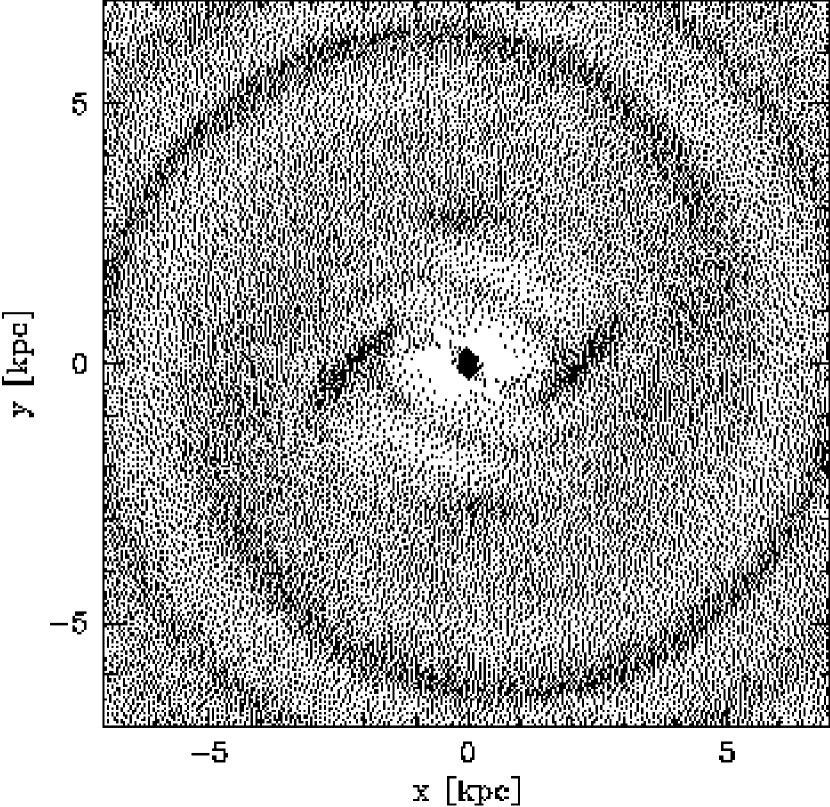
Figure 8: Gas flow in the same model as in Fig. 7, but with the density multipoles with $m\not=0$ set to zero outside $3{\rm\,kpc}$. Since the $l=0$ terms are unchanged, the circular rotation curve remains the same. The gas model extends to $10{\rm\,kpc}$ and has 20’000 particles.

Fig. 7 shows the morphology of the gas flow in this model. Inside corotation ($R_{c}=3.1{\rm\,kpc}$) two arms arise near each end of the bar. The dust lane shocks further in are barely resolved in this model. The structure into the corotation region is complicated. Outside corotation four spiral arms are seen. This four–armed structure is characteristic of all gas flow models that we have computed in the unmodified COBE potentials. A four–armed spiral pattern is considered by many papers the most likely interpretation of the observational material regarding the various spiral arm tracers and the five main spiral arm tangent points inside the solar circle (cf. Figs. 1, 2, Table 1), see the review and references in Vallée (1995).

Two of the four arms emanate approximately near the major axis of the bar potential, two originate from near the minor axis. The additional pair of arms compared to more standard configurations is caused by the octupole term in the potential; in a model where this term is removed, the resulting gas flow has only two arms outside corotation.

Fig. 8 shows the gas flow in a model in which the density multipoles with $m\not=0$ were set to zero outside $3{\rm\,kpc}$ before computing the potential. This modification leaves the circular rotation curve of the model unchanged. All structure in the resulting gas flow is now driven by the rotating bar inside corotation, whose quadrupole moment outside $R_{c}$ is weak. The figure shows that, correspondingly, only two weak spiral arms now form in the disk outside corotation. In the ($l,v$) diagram, these appear as tangents at longitudes $l\simeq-50^{\circ}$ and $l\simeq 50^{\circ}$. However, there are no arms in this model which would show along the tangent directions $l=\pm 30^{\circ}$; at best there are slight density enhancements in these parts of the disk. However, the abundance of warm CO clouds found near $l=25-30^{\circ}$ by Solomon, Sanders & Rivolo (1985; cf. Fig. 2) indicates that a spiral arm shock must be present in this region. Thus the model underlying Fig. 8, in which all structure in the gas disk outside $3{\rm\,kpc}$ is driven by only the rotating bar in the inner Galaxy, cannot be correct.

Both the quadrupole and octupole terms of the potential outside $\sim 3{\rm\,kpc}$ are dominated by the strong luminosity–mass peaks about $3{\rm\,kpc}$ down the minor axis of the COBE bar. From comparing Figs. 7 and 8 we thus conclude that, in order to generate a spiral arm pattern in the range $R=3-8{\rm\,kpc}$ in agreement with observations these peaks in the NIR luminosity must have significant mass. In other words, the NIR mass–to–light ratio in this region cannot be much smaller than the overall value in the bulge and disk. This result is in agreement with a recent study by Rhoads (1998) who finds that in external galaxies the local contribution of young supergiant stars to the NIR flux can be of order $\sim 33\%$ but does not dominate the old stellar population.

The observed luminosity peaks on the minor axis of the deprojected COBE bar coincide with dense concentrations of gas particles near the heads of the two strongest spiral arms in our gas model (Fig. 7). Since the gas arms will generally be accompanied by stellar spiral arms, this suggests that the most likely interpretation of the minor axis peaks in the BGS model is in terms of incorrectly deprojected spiral arms.

Spiral arms are generally the sites of the most vigorous star formation in disk galaxies. Also in the Milky Way, observations of far infrared emission show that most of the star formation presently occurs in the molecular ring (Bronfman 1992). Since we have found from dynamics that even in this region the associated young supergiants do not dominate the NIR light, this implies that over most of the Galactic disk the assumption of constant NIR mass–to–light ratio for the old stars is justified.

4.2 Time evolution

   

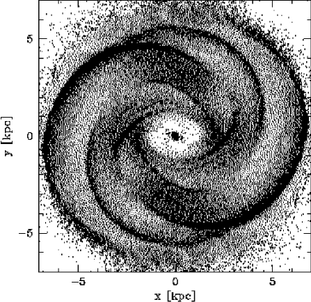
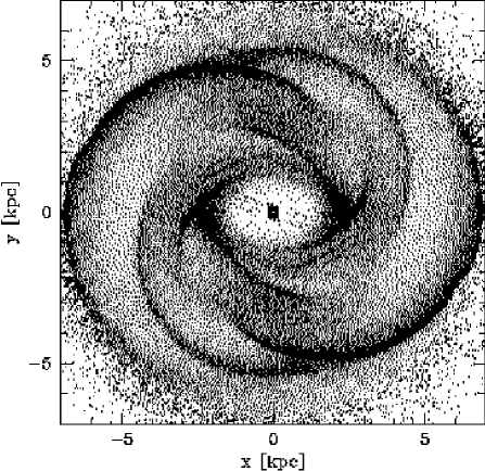
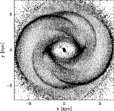
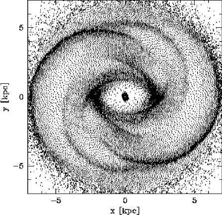
Figure 9: Gas particle distribution in the standard $\varphi_{\rm bar}=20^{\circ}$ COBE bar potential, for a corotation radius $R_{c}\simeq 3.4{\rm\,kpc}$. The frames show snapshots at $t=0.3{\rm\,Gyr},1.0{\rm\,Gyr},2.0{\rm\,Gyr},3.0{\rm\,Gyr}$ (top left, top right, bottom left, bottom right). The bar was gradually turned on between $t=0$ and $t=0.04{\rm\,Gyr}$. The particle rotation period at $3{\rm\,kpc}$ galactocentric radius is $\simeq 0.1{\rm\,Gyr}$. The most significant evolutionary effect is a loss of resolution by about a factor of two in linear distance between the first and the last frame, due to substantial mass inflow. This results in fuzzier spiral arms at the end of the simulation, which appear to terminate earlier. Also compare Fig. 10.

How stationary is the morphological structure in these gas flows? To address this question, we show in Fig. 9 the time evolution of a typical model ($\varphi_{\rm bar}=20^{\circ}$, $\Omega_{\rm P}=55\,\rm km\rm s^{-1}\rm kpc^{-1}$). In this and other simulations the non-axisymmetric part of the gravitational potential was gradually turned on within about one half of a bar rotation period ($\simeq 0.04{\rm\,Gyr}$). The gas flow, which is initially on circular orbits, then takes some time to adjust to the new potential. It reaches a quasi–stationary pattern by about time $t=0.3{\rm\,Gyr}$. This flow is shown in the top left panel of Fig. 9. After $t=0.3{\rm\,Gyr}$ the variations in the gas flow are small: about $5\,\rm km\rm s^{-1}$ in the velocities. Also the sharpness of the arms inside corotation varies slightly. In this quasi-stationary flow material continuously streams inwards: Gas parcels that reach a shock dissipate their kinetic energy perpendicular to the shock. Subsequently they move inwards along the shock.

As Fig. 9 shows, the inward gas inflow causes a slow evolution without much changing the morpophology of the gas flow. However, the mass accumulating on the central disk of $x_{2}$–orbits in the course of this process is considerable. In fact, to continue the simulation we have found it necessary to constantly remove particles from the $x_{2}$–disk. In doing this we have simultaneously increased the particle mass in this region in such a way as to keep the surface density unchanged. Therefore effectively we have only limited the resolution in this region from increasing ever further, without rearranging or changing mass. The gas inflow leads to a loss of resolution in the outer disk. From $t=0.3{\rm\,Gyr}$ to $t=3{\rm\,Gyr}$, the surface density of particles in outer disk of the model shown in Fig. 9 decreases by about a factor of four, i.e., the linear resolution by about a factor of two. The spiral arms therefore become more difficult to see; in particular, the starting points and end points of some of the arms appear to shift slightly.

The most rapid evolution occurs in the vicinity of the cusped orbit. Already by time $t=0.3{\rm\,Gyr}$, the gas disk near this orbit has been strongly depleted. Because the shear in the velocity field in the vicinity of the cusped orbit is very strong, particles that reach the cusped orbit shock move to the center quickly along the shock ridges and then fall onto the $x_{2}$–disk (Englmaier & Gerhard 1997). In the low-density region between the cusped orbit and the $x_{2}$–disk, the smoothing radius of the SPH particles is large compared to the velocity gradient scale. It is possible that the resulting large effective viscosity accelerates the depletion of gas on the cusped orbit and in its vicinity. A similar effect has been seen by Jenkins & Binney (1994) in their sticky particle simulations. See § 4.4 for an improved model with more resolution in the cusped orbit region.

4.3 Model (l,v)-diagrams

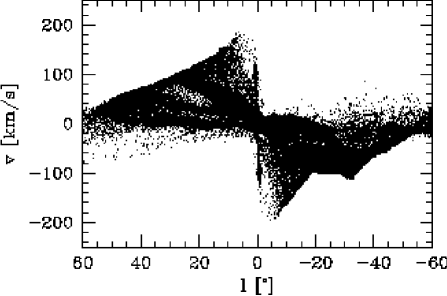
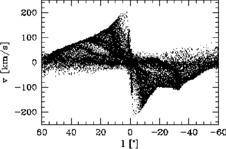
Figure 10: Longitude–velocity ($l,v$) diagrams corresponding to the gas particle distributions in Fig. 9 at $t=0.3{\rm\,Gyr}$ (top) and $3{\rm\,Gyr}$ (bottom). In constructing these we have assumed $R_{0}=8{\rm\,kpc}$ and $v_{0}=200{\rm\,km\,s^{-1}}$. The inner disk on $x_{2}$-orbits, the terminal velocity curve, and the spiral arm traces are apparent.

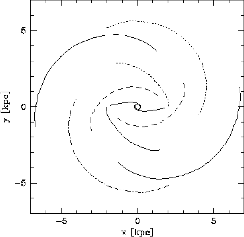
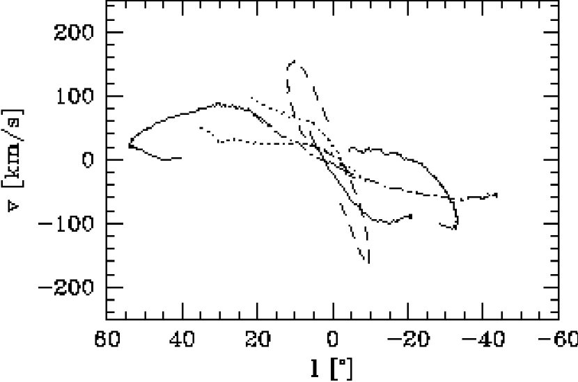
Figure 11: Top: Schematic representation of the spiral arms in the gas flow model depicted in the top left frame of Fig. 9. Bottom: The same spiral arms in the ($l,v$) diagram.

The non-axisymmetric structures seen in Figs. 9 etc. lead to perturbations of the gas flow velocities away from circular orbit velocities. These can be conveniently displayed in an ($l,v$) diagram like those often used for representing Galactic radio observations. In fact, to constrain the Galactic spiral arm morphology from comparisons of our models with Galactic radio observations, we really only have ($l,v$) diagrams! Fig. 10 shows ($l,v$) diagrams obtained from the gas distributions in the first and last panel of Fig. 9, at $t=0.3{\rm\,Gyr}$ and $t=3{\rm\,Gyr}$, respectively, for an assumed distance of the Sun to the galactic center of $8.0{\rm\,kpc}$ and LSR rotation velocity $v_{0}=200{\rm\,km\,s^{-1}}$. The bright ridge rising steeply from the center in these diagrams is caused by the dense disk of gas on $x_{2}$–orbits, visible in the very center of the flow in Fig. 9. The more irregularly–shaped ridges are the traces of spiral arms in the ($l,v$) diagram. Also well visible in Fig. 10 are the terminal velocity curves.

Looking at Figs. 9 and 10 shows that the relation between morphological structures in the gas disk and corresponding structures in the ($l,v$) diagram is somewhat non-intuitive. In order to gain a better understanding of this relation, we have constructed a schematic representation of the arm structures of the model in the top left panel of Fig. 9 in both coordinate planes. The upper panel in Fig. 11 shows schematically the location of the gaseous spiral arms, the cusped orbit shocks (dust lanes), and the $x_{2}$–disk in the ($x,y$)-plane. In this diagram, the Sun is located at $x=-7.5{\rm\,kpc}$, $y=-2.7{\rm\,kpc}$, i.e. at $R_{0}=8\,\rm kpc$ and $\varphi_{\rm bar}=20^{\circ}$. The lower panel shows the corresponding features in the ($l,v$) diagram as observed from this LSR position, with the same line styles to facilitate cross identification.

We see that whenever a spiral arm crosses a line–of–sight from the Sun twice, it appears as a part of a loop in the ($l,v$) diagram. This is the case, e.g., for the two outer spiral arms seen nearly end–on (thin full lines in Fig. 11), and for the innermost pair of arms driven by the bar (thick and thin dashed lines). The equivalent to the $3{\rm\,kpc}$ arm (see below) and the corresponding counterarm on the far side of the galaxy are parts of a second pair of arms driven by the bar; these cross the relevant lines–of–sight to the Sun only once (thick full lines and thick dotted lines in Fig. 11), respectively). The same is true for the outer pair of spiral arms seen nearly broad–on as viewed from the Sun (dash–dotted and small dotted lines).

It is clear from inspection of Figs. 10 and 11 and a comparison with the corresponding observational data (see the figures reproduced in Section 2, and the diagrams in the papers cited there) that already the initial COBE–constrained model gas flow of Fig. 9 resembles the Milky Way gas distribution in several respects:

(i) The number of arm features in the longitude range $[-60^{\circ},60^{\circ}]$ and their spacing in longitude is approximately correct (compare Table 1).

(ii) The model contains an arm which passes through the $l=0$–axis at negative velocity ($\sim-30{\rm\,km\,s^{-1}}$) and merges into the southern terminal velocity curve at negative $l$. Qualitatively, this is similar to the well–known $3{\rm\,kpc}$–arm, although this crosses the $l=0$–axis at $\sim-50{\rm\,km\,s^{-1}}$ and extends to larger longitudes.

(iii) The positions and velocities of gas particles in the $x_{2}$–disk are similar to those observed for the giant Galactic Center molecular clouds on the $l>0$ side in the CS line (Bally et al. 1987, 1988; Binney et al. 1991).

(iv) The terminal velocity curve slopes upwards towards large velocities near $l=0$, although not as much as would be expected for gas on and just outside the cusped orbit in the COBE potential (see § 4.4), and not as much as seen in the HI and CO data. In the following subsections we compare the COBE models more quantitatively with the observational data, and attempt to constrain their main parameters.

4.4 The terminal velocity curve

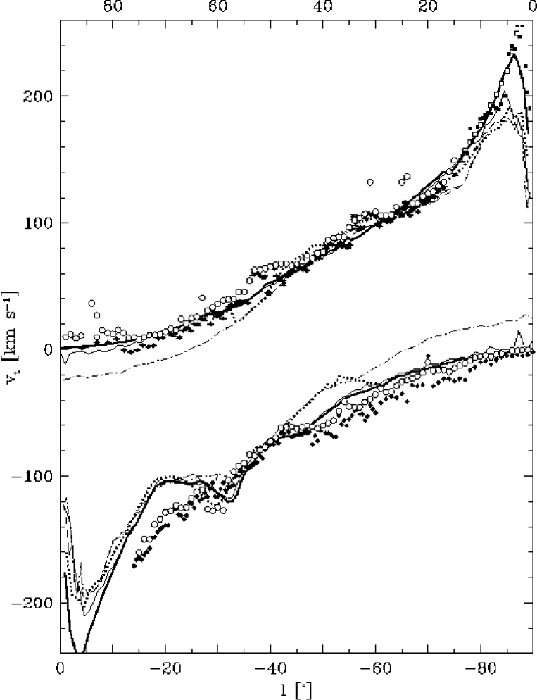
Figure 12: Northern and southern Galactic terminal velocity curves compared with model predictions. Observational data from sources as follows. Filled squares ($l=0-10^{\circ}$): HI data from Fig. 1 of Burton & Liszt (1993). Empty squares ($l=0-20^{\circ}$): unpublished 140ft single dish HI data, kindly provided by Dr. B. Burton. Open circles: HI terminal velocities from Fich et al. (1989), based on data from Westerhout (1957). Diamonds, with tiny error bars: northern ¹²CO terminal velocities from Clemens (1985). Without error bars: southern ¹²CO data from Alvarez et al. (1990). The data are relative to the LSR, mostly as corrected by the respective authors. The Clemens (1985) data have been corrected for internal dispersion, and the velocities in Burton & Liszt (1993) are relative to the Sun and have been corrected for LSR motion.    The model terminal velocity curves are from: a typical low resolution model with no halo and declining rotation curve (dash–dotted); the same model at higher resolution but with less radial extent (dotted); a low resolution model with flat rotation curve (thin solid); and our best model with high resolution (see text) and flat rotation curve (thick solid line). All models assume a bar angle $\varphi_{\rm bar}=20^{\circ}$ and have corotation at $R_{c}\simeq 3.4{\rm\,kpc}$.

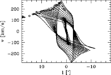
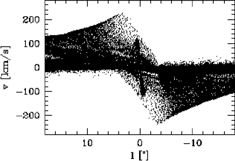
Figure 13: Top: The upper envelope of the $x_{1}$-orbits in the ($l,v$)-plane traces out the observed inner terminal velocity curve. The figure shows $x_{1}$-orbits computed in the same gravitational potential as that used for the models shown in Fig. 12; each $x_{1}$-orbit traces a parallelogram–like curve in this plot. The innermost $x_{1}$-orbit shown is the cusped orbit which peaks at $l=2^{\circ}$. Inside this orbit, the gas switches to $x_{2}$-orbits which reach velocities of $120\,{\rm\,km\,s^{-1}}$ in this potential. The observed northern terminal velocities are shown for comparison (same sources as in Fig. 12).    Bottom: Particle distribution in the same part of the ($l,v$)-plane, for the high–resolution model shown by the thick solid line in Fig. 12. The cusped orbit and the innermost few $x_{1}$-orbits are not occupied even at this resolution. The parallelogram structure in this plot therefore reaches inwards and upwards to only $l\simeq 3^{\circ}$ and $v\simeq 220{\rm\,km\,s^{-1}}$, compared to $l\simeq 2^{\circ}$ and $v\simeq 270{\rm\,km\,s^{-1}}$ for the orbits, and $l\simeq 2^{\circ}$ and $v\simeq 260{\rm\,km\,s^{-1}}$ for the observed terminal velocities.

We will now determine the mass normalisation of the models by fitting their predicted terminal velocity curves to observations. Model terminal curves are computed by searching for the maximal radial velocity along each line of sight, as seen from the position of the Sun $8{\rm\,kpc}$ from the center, and then substracting the projected component of the LSR motion. For the latter we have assumed that the LSR motion is along a circular orbit with $v_{\rm LSR}=200{\rm\,km\,s^{-1}}$ and no radial velocity component. By an eye-ball fit of these model curves to the observed terminal velocity curve we then obtain the proper scaling constant $\xi$ (see § 3.4) by which all velocities in the model have to be multiplied to obtain their Galactic values. Both the mass and the potential then scale with $\xi^{2}$.

Figure 12 shows several model terminal velocity curves obtained in this way, and compares them with the northern and southern Galactic terminal velocities as determined from HI and ¹²CO observations from a number of sources. Although the error bars for all measured terminal velocities are small, the data show some scatter due to differences in angular resolution and sensitivity. The model terminal velocity curves Fig. 12 are for models of different spatial resolution and simulated radial extent, to illustrate the effects of these parameters. The dash-dotted line is for a model extending to galactocentric radius $9{\rm\,kpc}$; this demonstrates that for $v_{\rm LSR}\geq 200{\rm\,km\,s^{-1}}$ the observed terminal curve beyond about $\pm(40-50)^{\circ}$ requires a dark halo component in the Milky Way.

After including a halo component in the model (by modifying the monopole component of the potential such that the rotation velocity becomes constant outside $4.5{\rm\,kpc}$; see Fig. 4), both the northern and southern terminal curves are much better reproduced (thick solid line in Fig. 12). The rotation curve of this halo model is shown in Fig. 4; the simulated radial range is $12{\rm\,kpc}$. The contribution of the dark halo inside the solar radius is fairly small ($\sim 23\%$ in the radial force at $8{\rm\,kpc}$), somewhat less even than in Kent’s (1992) maximum disk model.

In this model, there remain two main regions of discrepancy with the observed terminal velocity curve. First, the model terminal velocities are too low at and just outside the peak at $l\simeq 2^{\circ}$. This is strongly influenced by and probably due to resolution effects, as discussed below. Second, there is a larger mismatch around $-20^{\circ}$. This is likely caused by our mass model not being correct in the vicinity of the NIR lumps $\sim 3{\rm\,kpc}$ down the minor axis of the bar. Lines–of–sight at around $-20^{\circ}$ cross one of these lumps as well as the end of the $3{\rm\,kpc}$ arm and the head of one of the spiral arms outside corotation (see Fig. 11). The eight-fold symmetric deprojection of BGS is therefore likely to give incorrect results in this region. Smaller systematic deviations in the terminal velocities are visible around $l=30-50^{\circ}$ and $l=-(50-70)^{\circ}$, although there, and everywhere else, the differences between model and observations are now of the order of the scatter between the various observational data and of the order expected from perturbations in the disk. Given the uncertainties the overall agreement is surprisingly good. This suggests that the basic underlying assumption, that in the inner Galaxy the NIR light traces the mass, is mostly correct.

Fitting the terminal velocity curve to both sides we obtain a scaling constant of $\xi=1.12$. This is slightly larger than the value obtained in our first attempts to fit the models to the observations ($\xi=1.075$, Bissantz et al. 1997), in which we only considered the northern rotation curve and ignored the data beyond $l=48^{\circ}$. It is worthwhile pointing out that the derived value of $\xi$ is only weakly dependent on the assumed LSR tangential velocity: In order of magnitude, a $10\%$ change in the LSR velocity leads to a $1\%$ difference in $\xi$. With an improved dust model and deprojection of the outer disk we could therefore attempt to determine $V_{0}$ from these models.

As is clearly visible in Fig. 12, the peak in the observed terminal curve at $2^{\circ}$ is not well reproduced by our lower–resolution models. However, Fig. 13 shows that it is nicely approximated by the envelope of the $x_{1}$–orbit family when all orbital velocities are scaled by the same value of $\xi$. At early times in the model evolution, when the gas flow is not yet stationary, the peak is also reproduced in the hydrodynamic gas model, but thereafter the region around the cusped orbit is depopulated (see also Jenkins & Binney 1994). We attribute this to the artifical viscosity in the SPH method, which smears out the velocity gradient over two smoothing lengths, and to the method used for setting up the gas simulation.

We can estimate the magnitude of the effect as follows. Near the cusped orbit, which sets the maximum velocity along the terminal velocity curve, the particle smoothing length $h$ in the low resolution model is large, about $\sim 100{\rm\,pc}$, because the gas density in this region is small. The full $x_{1}$–orbit velocity on the terminal curve can only be reached about two smoothing lengths away from the cusped orbit, where it is no longer affected by the more slowly moving gas on $x_{2}$–orbits further in. The longitudinal angle corresponding to about $2h$ at the distance of the galactic centre is about $1.4^{\circ}$. Thus, the peak in the gas dynamical terminal curve should be found at $l>3.4^{\circ}$ when the orbits peak at $2^{\circ}$, showing how sensitive the peak location is to resolution.

To test this explanation, we have run a bi-symmetric model with $100,000$ particles, resulting in about 2.2 times as much spatial resolution as in the low–resolution models. Just on the basis of this higher resolution, the terminal velocity peak then moves from about $5^{\circ}$ to $4^{\circ}$ (at $t=0.3\,\rm Gyr$). We then further increased the resolution by the following procedure. The gas inside the outermost $x_{1}$ orbit shown in Fig. 6 was removed, and set up again on nested closed $x_{1}$ and $x_{2}$ orbits, while keeping particles outside this region unchanged. Evolving this modified gas distribution for a further $0.3\,\rm Gyr$, we obtained our final high resolution model. This is shown by the thick solid line in Fig. 12, which peaks at about $3^{\circ}$ and $v_{t}=235{\rm\,km\,s^{-1}}$. Compared to the original $20000$ particle model (thin solid line in Fig. 12) the mismatch at the peak has been reduced by about a factor of two in scale and by two thirds in the peak velocity.

Although this analysis was inspired by a technical problem, there is an observable implication of it as well. Since we may interpret the hydrodynamical model in terms of gas clouds having a mean free path length of order the smoothing length, we may restate the result in the following way: a loss of resolution occurs when the cloud mean free path is significant compared to the gradient in the true velocity field. Applied to the inner Galaxy, our result then indicates that the clouds near the cusped orbit peak in the terminal velocity curve must have short mean free paths, i.e., be described well in a fluid approximation.

Apart from resolution effects, the precise position of the peak in the terminal velocity curve also depends critically on the location of the ILR and hence on the mass model in the central few $100{\rm\,pc}$. In this region, the deprojected COBE model suffers from a lack of resolution and our added nuclear component has uncertainties as well. We therefore believe that with improved data and further work the remaining discrepancies in this region will be fixed.

4.5 Pattern Speed and Orientation of the Galactic Bar

     

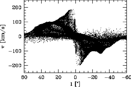
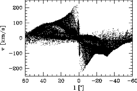
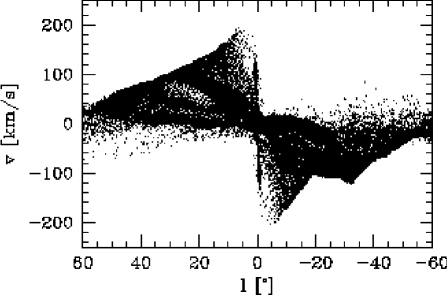
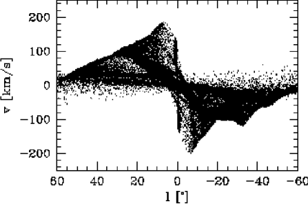
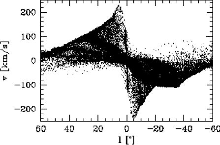
Figure 14: Longitude–velocity ($l,v$) diagrams for the gas flows in COBE bar potentials with different pattern speeds and bar orientation angles. The column of ($l,v$) diagrams on the left shows the influence of the pattern speed on the gas flow in the standard $\varphi_{\rm bar}=20^{\circ}$ COBE bar potential. These frames show models with corotation radii $R_{c}=3.1{\rm\,kpc}$ (top) $R_{c}=3.4{\rm\,kpc}$ (middle) to $R_{c}=4.0{\rm\,kpc}$ (bottom). The right column shows gas flows in COBE bars deprojected for different bar orientation angles, $\varphi_{\rm bar}=15^{\circ}$ (top), $\varphi_{\rm bar}=25^{\circ}$ (middle), $\varphi_{\rm bar}=30^{\circ}$ (bottom), all for corotation at $R_{c}=3.4{\rm\,kpc}$.

There are two observations which constrain the value of the pattern speed rather tightly. First, there is the 3-kpc-arm, a feature which exhibits non-circular motions of at least $50\,\rm km\rm s^{-1}$. In our models, we find that only the arms inside the bar’s corotation radius are associated with strong non-circular motions, so such an arm has to be driven by the bar. From observations and models of barred galaxies we also know that strong spiral arms associated with both ends of a bar are common. Therefore we conclude that the 3-kpc-arm must lie inside the bar’s corotation radius.

Second, a lower limit to the corotation radius is given by the inner edge of the molecular ring. If the molecular ring were indeed a ring such as induced by a resonance, it would be located near the outer Lindblad resonance (e.g., Schwarz 1981). On the other hand, if it is actually made of several spiral arms (Dame 1993, Vallée 1995, this paper), then the small observed non-circular velocities along these spiral arms also show that these arms must be outside the bar’s corotation radius. Solomon et al. (1985) find from the distribution of hot, presumely shocked cloud cores, that the inner edge of the molecular ring is at $R=4\,\rm kpc$. The total surface density of neutral gas also drops dramatically inside of $4{\rm\,kpc}$ (Dame 1993). From the IRT $2.4\,{\mu\rm m}$ photometry of the galactic disk Kent et al. (1991) concluded that there is a ring, or spiral arm, at about $R=3.7\,\rm kpc$. Therefore we conclude that the bar’s corotation radius is inside $R=4\,{\rm\,kpc}$.

An independent argument for corotation falling somewhere between $3{\rm\,kpc}$ and $4{\rm\,kpc}$ comes from the fact that the deprojected COBE bar appears to end somewhere between $3{\rm\,kpc}$ and $3.5{\rm\,kpc}$ (BGS). From both N–body simulations and direct and indirect observational evidence the corotation radius is usually found at between 1.0 and 1.2 times the bar length (Sellwood & Wilkinson 1993; Merrifield & Kuijken 1995; Athanassoula 1992b). In our models, a coration radius between $3{\rm\,kpc}$ and $4\,\rm kpc$ corresponds to a pattern speed of $\sim 50-60\,\rm km\rm s^{-1}\rm kpc^{-1}$.

We have run gas dynamical simulations with corotation at 4.0, 3.4, and $3.1\,\rm kpc$, to determine from observations which of these values is most nearly appropriate. For the comparison with observations it is important to notice that several other parameters enter here, most importantly, the orientation angle of the bar, the uncertain contribution of the dark halo to the outer rotation curve and hence terminal velocities, and the LSR velocity.

We first fix the bar orientation angle at $\varphi_{\rm bar}=20^{\circ}$, but will vary this parameter later. The chosen value of $\varphi_{\rm bar}$ is in the range allowed by the NIR photometry (BGS), it is favoured by the clump giant star distribution as analyzed by Stanek et al. (1997) and by the gas kinematical analysis of the molecular parallelogram by Binney et al. (1991), and it meets the preference for an end–on bar in the interpretation of the microlensing experiments.

In the last section we found that the Galactic terminal velocity curve for $|l|\leq 45^{\circ}$ is well–reproduced by the gas flow in the maximum NIR disk model with constant mass–to–light ratio. Moreover, even this maximum disk model fails by a factor of $\mathrel{\hbox to0.0pt{\lower 3.0pt\hbox{$\mathchar 536\relax$}\hss}\raise 2.0pt\hbox{$\mathchar 318\relax$}}2$ in explaining the high microlensing optical depth towards the bulge (Bissantz et al. 1997), making it very difficult to further reduce the mass in the intervening disk and bulge. We can therefore confidently assume a maximum disk model in the following and, to separate the determination of the bar and halo parameters, we restrict the comparison with observations to longitudes $|l|\leq 45^{\circ}$.

Finally, we set the LSR rotation velocity to $V_{0}=200{\rm\,km\,s^{-1}}$, in the middle of the observed range (§2.7). A $10\%$ difference in this parameter is not very important for the comparison with the inner Galaxy gas velocities.

Thus we begin by considering a sequence of models with varying corotation radius $R_{c}$ and the other parameters fixed as just described. For three models with $R_{c}=4.0{\rm\,kpc}$, $3.4{\rm\,kpc}$, and $3.1\,\rm kpc$ we have plotted (l,v) diagrams and have determined the scaling constant $\xi$ for each simulation by fitting to both terminal curves. The final scaled ($l,v$) diagrams are shown in the left column of Fig. 14. For the scaling constant we obtain $\xi=1.13$, 1.12, and 1.09 for the 4.0, 3.4, and $3.1{\rm\,kpc}$ models. The correctly scaled pattern speeds are then $59$, $57$, and $61\,\rm km\rm s^{-1}\rm kpc^{-1}$. This means that by changing the corotation radius, we effectively change the mass of the model galaxy, while keeping the pattern speed almost constant at about $60\,\rm km\rm s^{-1}\rm kpc^{-1}$.

At small absolute longitudes, $|l|\leq 10^{\circ}$, these low–resolution models do not have enough particles to resolve the true gas flow, and furthermore there are no published terminal velocities in this region on the southern side. Thus for now we ignore data near the peak of the terminal velocity curve. This leaves a range of $\pm l=10-45^{\circ}$ within which we compare these no–halo model gas flows with the northern and southern terminal velocity curves and with the various spiral arm features shown in Figs. 1–2.

On the northern side ($l>0$), we try to match the model to the pronounced spiral arm at about $+30^{\circ}$, which is best visible in the warm CO clouds (Solomon et al. 1985) and in the distribution of HII-regions. Moreover, the (l,v)-diagrams of CO and HII-regions shows that the $+30^{\circ}$ arm is double (Fig. 2). In the model shown schematically in Fig. 11, there are actually three arms near $l\simeq 30^{\circ}$, two of which overlap, while the third, the northern 3-kpc-arm (thick dotted line), runs almost parallel to the first two. There is also a wiggle in the terminal curve at about $+10^{\circ}$, which is probably caused by a spiral arm similar to the northern, secondary inner spiral arm in the model (thin dashed line in Fig. 11). The southern terminal curve is more distorted by spiral arms than the northern curve. A pronounced feature is the $-30^{\circ}$ arm in the molecular ring, as well as the well–known 3-kpc-arm which continues on from a non–circular velocity ridge beginning at $l\simeq 10^{\circ}$ and $v=0$.

Fig. 14 (left column) shows that the gas flows in all three cases are similar; nonetheless small differences in the spiral arm locations help to show that the $3.4\,\rm kpc$ case is closest to the real Galaxy. The $30^{\circ}$ spiral arm tangent is best reproduced in the $3.4{\rm\,kpc}$-model (middle panel in left column of Fig. 14). In the top panel, it is not double as observed, and in the bottom panel the tangent moves out to $\sim 40^{\circ}$. The $50^{\circ}$ spiral arm tangent is reasonably well reproduced in the top two panels, but is absent or very weak in the bottom panel, but this arm may not be a reliable indicator in the absence of a halo. In the south, we observe that large corotation radii move the arm at $-30^{\circ}$ outwards. The $-30^{\circ}$ spiral arm tangent is in about the correct location in the top two panels, but too far out in the bottom panel. The mismatch of the terminal curve at about $-20^{\circ}$ becomes larger with decreasing corotation radius as well. On the other hand, the $-50^{\circ}$ spiral arm tangent is not present for the largest pattern speed (top panel), while it is adequately present in the lower two panels. The 3-kpc-arm equivalent is present in all three models, but its detailed locus in the ($l,v$) diagram is not correct in any of the models: it has either too low non–circular velocities at $l=0$ (particularly in the bottom panel), or it does not extend to large enough negative longitudes (particularly in the top panel). For corotation at $3.4{\rm\,kpc}$, the 3-kpc-arm ends in the model exactly at $3\,\rm kpc$, as seen from the assumed solar position. There are particles in the low intensity forbidden velocity region bounded by the line from $(l,v)=(10,0)-(0,-50)$ in all three models, but the resolution does not suffice to prefer one model over the other. Finally, an equivalent to the $155{\rm\,km\,s^{-1}}$ arm at small negative $l$ is present only for the lowest pattern speed.

From an unweighted average of these comparisons to various observational landmarks we conclude that the corotation radius of the Galactic bar is most likely at about $3.4\,\rm kpc$. However, since none of the above models is exactly right yet, this value could well change by $10\%$ when other effects are taken into account, such as bar orientation (discussed next), dark halo (§4.6), or self–gravitating spiral arms (§4.7).

With the corotation radius fixed at $3.4\,\rm kpc$, we can attempt to find an optimal orientation angle for the bar. For this purpose, a series of deprojected bar models have been made as in BGS, for bar orientation angles $\varphi_{\rm bar}=10$, 15, 20, 25, and $30^{\circ}$. Smaller or larger angles are not consistent with the asymmetry pattern of the observed NIR distribution or result in unphysical bar shapes, see BGS and Bissantz et al. (1997). With the bar orientation the shape and radial extent of the deprojected bar change.

Gas flow simulations with $R_{c}=3.4\,\rm kpc$ were made for each of these cases, and ($l,v$) diagrams for $\varphi_{\rm bar}=15$, 25, and $30^{\circ}$ are shown in the right column of Fig. 14. We observed that the resulting changes in the model terminal velocity curves are caused in about equal parts by the change in the viewing direction relative to the bar, and by the intrinsic differences between the deprojected mass distributions. The models’ scaling factors $\xi$ are again determined separately for each model by eyeball fitting the observed northern and southern terminal curves. The variation in $\xi$ is very small, however: we obtain $\xi=1.1$, 1.11, 1.12, 1.11, and 1.12 for orientation angles from $10^{\circ}$ to $30^{\circ}$.

We find only a weak preference for the $20^{\circ}$ model. The $-30^{\circ}$ arm is more consistent with the $10^{\circ}$ and $15^{\circ}$ case, whereas these models show too large terminal velocities around $+40^{\circ}$. The $+30^{\circ}$ arms seem to be in favour of $15-25^{\circ}$, whereas the 3-kpc-arm, although always too slow at $l=0$, seems to fit slightly better with $20^{\circ}$. We conclude that the orientation is about $20^{\circ}$ with a large uncertainty.

4.6 Spiral arm tangents

 

 

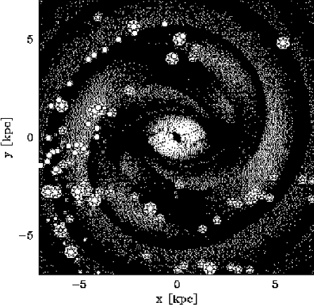
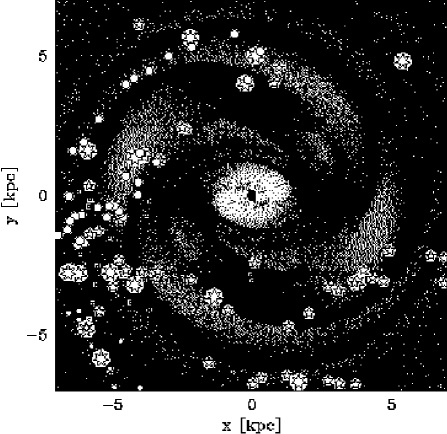
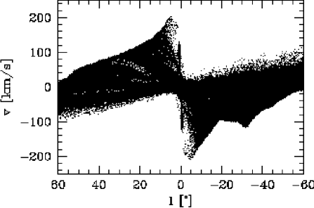
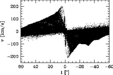
Figure 15: Spiral arm tangents in two models with $\varphi_{\rm bar}=20^{\circ}$ compared to observations. Left: standard model without dark halo; right: including dark halo. Both models are computed with 100,000 particles and the gas disk is truncated at $10{\rm\,kpc}$. The observed directions of spiral arm tangents are shown by the straight lines, starting at the position of the Sun at $x=-7.5{\rm\,kpc}$, $y=-2.7{\rm\,kpc}$ in this plot. See Table 1 which also lists the spiral arm tangents for the models. For illustration, stars denote positions of major HII-Regions from Georgelin & Georgelin (1976) and Georgelin et al. (1996), and circles the positions of large molecular clouds from Dame et al. (1986) and Grabelsky et al. (1988). The distances of these tracers have been rescaled to $R_{0}=8{\rm\,kpc}$ but are not corrected for non-circular motions. Such a correction would tend to move HII-Regions into the model spiral arms, because of velocity crowding.

In the previous §4.5 we have already used the observed spiral arm tangents at $l=\pm 30^{\circ}$ to constrain the pattern speed and orientation angle of the bar. Here we reconsider the location of the spiral arms in the models that compared best with the Galaxy in §4.5 (i.e., those with $R_{c}=3.4{\rm\,kpc}$ and $\varphi_{\rm bar}=20^{\circ}$), but with (i) a possible dark halo included, (ii) emphasis also on the nearby terminal curve and the spiral arms with tangents at $l=\pm 50^{\circ}$, and (iii) higher resolution.

For comparing the model spiral arms with observations we again use the tracers in Fig. 2 (HII regions and molecular clouds) and the characteristic features in ($l,v$) diagrams like Fig. 1. Unfortunately, because the structures in the observed ($l,v$) diagrams are much less sharp than in the model ($l,v$) diagrams, it is very difficult to measure reliably any features beyond those already discussed, i.e., the spiral arm tangent point positions, the 3–kpc arm and the molecular ring. Already the run of the arms out of the molecular ring to their tangent points cannot be identified unambiguously from Fig. 1.

Spiral arm tangent directions in the models are easily determined. When the arm is broadened in the tangential direction, we place the tangent at the outer edge, where the velocity jump is. In this way we can achieve a fair accuracy of a few degrees. Only one tangential direction, the Scutum arm at $l=30^{\circ}$, cannot easily be determined in this way, because its tangent goes through the corotation region through which no arm continues inwards in the model. Nevertheless, we can measure an approximate value for this tangent as well. Table 1 gives a comparison of model and observed spiral arm tangent directions, and the various data that have been used for the observed directions.

The bar–driven spiral arms in the models change their relative strength, opening angle, and hence location, depending on pattern speed, bar orientation, halo mass contribution and other parameters. In §4.5 we have discussed the constraints on the the pattern speed and bar orientation angle. Fig. 15 shows that adding a dark halo mass contribution so as to make the outer rotation curve flat (at $208{\rm\,km\,s^{-1}}$ after scaling) has the following two effects: (i) the outer pair of spiral arms at $l=\pm 50^{\circ}$ now form a more regular pattern with the inner pair at $l=\pm 30^{\circ}$, and all four arms now have a similar density contrast with respect to the interarm gas; (ii) all four tangent directions now fit the observations reasonably well; see also Table 1. Fig. 15 also shows the positions of large HII-regions and molecular clouds superposed on the gas arms. Note that their distances were determined from a circular orbit model and so may be slightly in error. Nonetheless it is reassuring that they fall approximately on the model gas arms, consistent with the model’s match to the spiral arm tangents.

4.7 Gravitating spiral arms

   

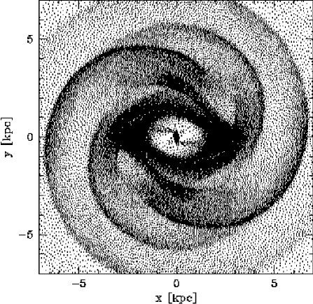
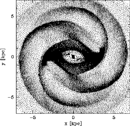
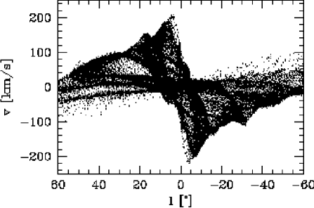
Figure 16: Model with additional spiral arm potential. Left: case with realistic parameters; right: twice as high surface density, and half as large gravitational smoothing lengths.

In this section we estimate the effect, if any, of the gravitational potential of the stellar spiral arms that are likely associated with the spiral arms seen in the gas. Remember that in our model, the spiral arms outside the bar’s corotation radius are driven by the clumps of NIR light and mass $\sim 3{\rm\,kpc}$ down the minor axis, which rotate with the bar (see §4.1). We interpret these clumps as the signature of real spiral arms in the deprojected NIR light. In the gas model two of the spiral arm heads are about at the correct positions where these clumps are observed; this supports the view that the gravitational potential of the clumps is a first estimate of the true spiral arm potential.

However, the models discussed sofar did not take into account the gravitational perturbations outside the clump regions that could be associated with the spiral arms. In particular, we are interested in knowing whether the morphology of the spiral arms would be changed when these arms carry a reasonable fraction of the mass throughout the disk. To test this, we have experimented with the following scheme that makes use of the particular strengths of the SPH method: First, we assign a fraction of the mass of the NIR disk to the spiral arms. Most of this mass will be associated with the spiral arm perturbation in the stellar density. Then we assign this part of the mass to the gas particles, assuming that a large fraction of the gas will later be concentrated in the arms and that the shock fronts seen in the gas will trace the stellar spiral arm crests. Finally, to mimic the fact that the stellar spiral arms are much broader in azimuth than the shocks seen in the gas, we set the gravitational softening radius of the gas particles to a value appropriate for the stellar arm widths and different from the smoothing length used in the calculation of the hydrodynamic forces.

According to Rix & Zaritsky (1995), the spiral arms cover about one third of the surface area in galaxies morphologically similar to the MW. The arm–interarm contrast is somewhat less than average for these galaxies, so that we estimate that about $20\%$ of the total NIR luminosity is in the spiral arms (superimposed on the axisymmetric background disk which thus contributes about $80\%$).

The azimuthally averaged surface density associated with the spiral arms should thus also be $\sim 20\%$ of the mean background stellar surface density. In the solar neighborhood, the stellar surface density of our normalized models is $35\xi^{2}M_{\odot}{\rm\,pc}^{-2}$. Thus we first take an ‘arm’ potential corresponding to a mean surface density of $7M_{\odot}{\rm\,pc}^{-2}$ at the solar radius, and a factor $\exp[-(r-8{\rm\,kpc})/2.5{\rm\,kpc}]$ more further in. Here we have used the radial scale-length of the NIR disk from §3. This spiral arm mass is given to the gas particles, and in order to compensate for the extra mass, we substract the same amount as a constant fraction from the COBE NIR mass model.

Because the stellar spiral arms are less sharp than gaseaus arms, we estimate their gravitational force by smoothing the gravitational forces of the gas particles over some length scale $\varepsilon$. Each particle contributes a smoothed potential

$$\phi_{i}({\mn@boldsymbol{r}})=-{Gm_{\ast i}\over\sqrt{({\mn@boldsymbol{r}}-{\mn@boldsymbol{r}}_{i})^{2}+\varepsilon^{2}}}$$ (5)

to the gravitational field of the ‘arms’. Here, $m_{\ast i}$ denotes the stellar mass associated with particle $i$; $m_{\ast i}$ is obtained by dividing the total mass in the stellar spiral arms by the effective number of gas particles. The parameter $\varepsilon$ must depend on the average distance between two arms in the model (about $3{\rm\,kpc}$ in the region of interest). We thus mimic the broader spiral arm potential by smoothing the gas arm potential over about $\varepsilon\sim 1\,{\rm\,kpc}$.

Notice that the hydrodynamical forces do not depend on the actual value of the surface mass density, but only on the particle density gradient. We can therefore save some memory space by taking the SPH particle mass $m_{i}$ equal to the stellar $m_{\ast i}$.

The initial gas disk is set up in a similar way as for the models discussed above, but for consistency the surface density is that of an exponential disk with the same radial scale length as the stellar disk. The resulting additional radial pressure gradient is far to weak to change the dynamics.

In our first attempt at such a model we found that the mass in the gas particles accumulating on the $x_{2}$-disk due to inflow was so large that the rotation curve in this region was changed significantly. Moreover, the dust lane shock fronts acquired significant mass. This is unrealistic since no strong stellar arms form at the edge of the bar, and it has the effect of changing the gas flow near the cusped orbit. To avoid both effects we have set the gas particle masses to zero inside the bar region, which was approximated by an ellipse with major axis $3{\rm\,kpc}$ and minor axis $1.8{\rm\,kpc}$. Correspondingly, the COBE mass model was then not changed in this region.

The gravitating arm model with the specified parameters that finally results is shown in the left panels of Fig. 16. First, we notice that the distribution of gas has not changed much compared to Fig. 15. Especially the locations of the arms are unchanged. The inner arms now contain more particles, because of the initial exponential surface density profile. However, the line–of–sight velocities have been modified somewhat. For example, the 3-kpc-arm has now about the right velocity: $\simeq-41{\rm\,km\,s^{-1}}$ at $l=0$. At around $l=20^{\circ}$ the terminal velocities are now larger than the observed velocities. On the southern side, at $l\sim-20^{\circ}$, the velocities are also higher, removing part of the previous discrepancy between model and observation. The larger velocities in this region are probably due to the mass in the 3-kpc-arm and the second arm at $\sim 2{\rm\,kpc}$ and their symmetric counterarms.

We have also run a model with about twice as much mass in the ‘arm’ potential and half the smoothing length, $\varepsilon=0.5{\rm\,kpc}$ (right panels of Fig. 16). Both parameter increase the gravitational response to the arms and are extreme values for the Milky Way. In this case, the distribution of the gas has changed more dramatically, especially in the region close the the bar. The inner arms seem to form an ellipse around the bar; however, the number of arms has still not changed. The 3-kpc-arm in this model is faster than the observed 3-kpc-arm and expands with $60{\rm\,km\,s^{-1}}$ towards the observer at $l=0$, but it no longer extends out to $3{\rm\,kpc}$. The model terminal curve now gives only a poor fit to the observations. One interesting property of this model is that it contains much more gas with forbidden velocities than all our other models.

From both models it is clear that the gravitational potential of the spiral arms is important for the comparison with Galactic ($l,v$) diagrams at a level of $\sim 15{\rm\,km\,s^{-1}}$. Especially the 3-kpc-arm and details in the terminal velocity curve depend on this parameter. Besides that, however, the morphology and spiral arm tangents are not effected much. It is encouraging that the inclusion of spiral arm gravity appears to improve the fit to some aspects of the data, even though the models discussed in this section certainly do not contain the entire story. For example, we have not subtracted a fraction of the mass in the minor axis NIR clumps which should now be taken care of by the spiral arms. On a more fundamental level, it is quite possible that the spiral arms between the bar and the solar circle rotate with a somewhat different pattern speed from that of the bar (see Sellwood & Wilkinson 1993 for a review of this subject, and Amaral & Lépine 1997 for a separate model of the Galactic spiral arms with a slow pattern speed). If this were the case, we would have to observe the resulting time–dependent pattern of bar and spiral arms at a moment when both the apparent NIR distribution of light and the induced kinematical perturbations resemble those observed in the Milky Way. This may not be as difficult as it appears because of the Galaxy’s relatively tightly wound four–armed spiral pattern. However, simulating this would introduce an entirely new degree of freedom and will not be attempted here.

5 Conclusions

We have presented a new set of hydrodynamical models for the gas flow in the Galactic disk inside the solar circle. These gas flows are evolved in the gravitational potentials obtained by deprojecting the NIR luminosity distribution of the Galactic bar and disk from COBE/DIRBE under the assumption of eight–fold symmetry (as in Binney, Gerhard & Spergel 1997), assuming constant mass–to–light ratio for the NIR luminous material, and adding a nucleus and (in some cases) a dark halo component. These models allow us to understand many features of Galactic HI and CO observations.

To follow the gas dynamics we have used the Smooth Particle Hydrodynamics (SPH) code described in Englmaier & Gerhard (1997). With the SPH method we can resolve the spiral arm shocks well, and use them in some models as tracers for the gravitational potential of the stellar spiral arms. The hydrodynamical models quickly settle to an approximate quasi–equilibrium flow pattern whose overall morphology is not sensitive to the precise value of the bar’s pattern speed, to the orientation of the bar with respect to the observer, and to whether or not the spiral arms carry mass.

We have compared our gas models with Galactic HI, CO, HII, and other data. We find that these models provide a coherent explanation of many aspects of the data, such as: (i) the four–armed spiral structure of the Milky Way between corotation and the solar radius, (ii) the nature of the 3–kpc–arm, (iii) the terminal velocity curve, (iv) the non–circular velocities near the cusped orbit at the ILR, and (v) the disk of gas on the inner $x_{2}$–orbits. Thus NIR photometry and gas kinematic observations conform to a single picture, and the Galactic bar is an essential part of this.

In this picture, the bar (bulge) rotates with a pattern speed such that corotation is at $R_{c}\simeq 3.5\pm 0.5{\rm\,kpc}$. The 3-kpc arm is one of the arms emanating from the ends of the bar, extending into the corotation region. Outside corotation, a four–armed spiral arm pattern gives rise to the molecular ring and the arms extending to the solar circle and beyond. In the model, this pattern is generated by the rotating luminosity/mass concentrations on the bar’s minor axis found by BGS. These can therefore not just be due to light from young supergiant stars, but must be massive; most likely they are symmetrized approximations to the stellar spiral arms themselves. A spiral pattern similar to that found here has been observed by Fux (1998) in those of his N–body – SPH barred galaxy models which compare best to the Galactic ($l,v$) diagrams. These models start from a set of specified initial conditions rather than from observations. The fact that both approaches lead to similar overall results is encouraging.

We find that the Galactic terminal curve out to longitudes $l\simeq 45^{\circ}$ is consistent with a maximal, constant mass–to–NIR light disk and bar model. The inferred mass in the disk cannot easily be reduced because (i) this model still underpredicts the microlensing optical depth towards the bulge (Bissantz et al. 1997) and (ii) it predicts about the correct surface mass density for the old stellar disk near the Sun. Thus the Galactic dark halo will be an important contribution to the mass of the Milky Way only outside of at least $R=5{\rm\,kpc}$, depending on the LSR rotation velocity.

The models are similar and in reasonable overall agreement with the Milky Way observations for a range of values of the bar’s orientation angle. Probably best is $\varphi_{\rm bar}=20-25^{\circ}$ but the uncertainties are are such that $15^{\circ}$ or $30^{\circ}$ cannot be excluded. The detailed match to various key observational quantities does depend on $\varphi_{\rm bar}$ and the precise value of $R_{c}$, but at a level comparable to the influence of various other parameters including the LSR rotation velocity, the asymptotic halo circular speed, and the influence of the stellar spiral arm gravity.

Some features of the HI and molecular emission data can be reproduced quantitatively, such as the Galactic spiral arm tangent positions, much of the terminal velocity curve, or the position of the nuclear $x_{2}$–disk. On the other hand, a detailed quantitative fit to all features in the observed ($l,v$) diagrams is not yet possible. The 3-kpc arm in the model has the correct angular extent but somewhat too small non-circular velocities. Its arm tangent position coincidences with the place where the model terminal curve differs most from the observations. In this region the disk mass model may not be very accurate. The position and velocity of the molecular parallelogram are fitted well by closed orbits in the NIR potential, whereas the hydrodynamic gas flow underestimates the velocity and overestimates its radial scale. Probably both hydrodynamic resolution and uncertainties in the potential near $\sim 200{\rm\,pc}$ (where the NIR data have insufficient resolution) are responsible for this. Also, this suggests that the clouds near the peak of the terminal velocity curve have a small mean free path.

Much work remains to be done. Because the deprojected disk model accounts only insufficiently for the Galactic spiral arms, some aspects of the gravitational potentials used are likely to be wrong. With a model for the spiral arms in hand, both the correction of the NIR data for dust and the subsequent deprojection of these data could be improved. Further observational work on spiral arm tracers such as HII regions and molecular clouds would be highly valuable for clarifying the run of the weaker Galactic spiral arms and those on the other side of the bar, and thus for better constraining the gas-dynamical models. Distance estimates to these tracers could be improved by making use of the velocity fields in these models.

On a more fundamental level, several assumptions made in the models may be or are likely to be invalid at some level, and require further study: (i) that the gravitational potential and gas flow structures are quasi-stationary and point–symmetric with respect to the Galactic Centre; (ii) that the NIR light is a fair tracer of the stellar mass, i.e., that young supergiant stars do not contribute significantly to the NIR light (but see Rhoads 1998); (iii) that the gas disk can be treated as planar; (iv) and that the bar and spiral arms rotate with the same pattern speed.

6 Multipole expansion

For the SPH simulations, the gravitational forces are calculated using a multipole expansion of the stellar density model. The stellar density is given by

$$\rho(r,\theta,\varphi)=\rho_{0}f(r,\theta,\varphi)$$ (6)

where the function $f$ is the interpolated deprojected light distribution within the bulge region and the exponential disk elsewhere. Here, the constant $\rho_{0}$ is the presently unknown unit of luminosity density multiplied by the also unknown mass-to-light ratio. A first estimate gives $\rho_{0}=\xi^{2}3\;10^{8}\;M_{\odot}/\rm pc^{3}$, where $\xi$ is of the order of unity and is measured by fitting the observed rotation velocity in § 4.4.

The density multipoles

$$\rho_{lm}(r)=\int_{0}^{\pi}\!\!{\rm d}\theta\sin(\theta)P_{lm}(\cos(\theta))\int_{0}^{2\pi}\!\!{\rm d}\varphi\cos(m\varphi)f({\mathbf{r}})$$ (7)

satisfy the identity equation

$$\rho({\mathbf{r}})=\sum_{l,m}(2-\delta_{m0}){(2l+1)(l-m)!\over 4\pi(l+m)!}\rho_{lm}P_{lm}\cos(m\varphi).$$ (8)

The $P_{lm}$ are the associated Legendre functions. Here we have used that $f$ is an even function in $\phi$: $f(r,\theta,\phi)=f(r,\theta,-\phi)$, and have restricted the sum to positive $m$.

Both integrations were performed with the Romberg method. The density multipoles $\rho_{l0}$ were then fitted to a power law $C_{l}r^{p_{l}}$ in the range of $350\;\rm pc$ to $500\;\rm pc$ with the method of least squares. The tabulated multipole expansions were then replaced by the fit inside $350\;\rm pc$.

From the modified tables $\rho_{lm}(r)$ we calculated the following two auxiliary integrals:

$$I_{<}(r)=\int_{0}^{r}{\rm d}a\,\rho_{lm}(a)a^{l+2}$$ (9a)

and

$$I_{>}(r)=\int_{r}^{\infty}{\rm d}a\,\rho_{lm}(a)a^{1-l}$$ (9b)

For stability reasons we used for these integrations the trapezoidal rule on the 3000 logarithmically equidistant $\rho_{lm}$ values tabulated between $1\;\rm pc$ and $12\;\rm kpc$. The region between $12$ and $16\;\rm kpc$ in the second integral was calculated again with the Romberg method; outside $16\;\rm kpc$ the density was set to zero.

From this, we get the potential multipoles

$$\Phi_{lm}(r)=(2-\delta_{m0}){(l-m)!\over(l+m)!}(r^{-l-1}I_{<}(r)+r^{l}I_{>}(r))$$ (10)

as well as their first derivatives

$$\Phi^{\prime}_{lm}(r)=(2-\delta_{m0}){(l-m)!\over(l+m)!}(-(l+1)r^{-l-2}I_{<}(r)+l\;r^{l-1}I_{>}(r)).$$ (11)

The potential is then given by

$$\Phi(r)=-G\rho_{0}\sum_{l,m}\Phi_{lm}(r)P_{lm}\cos(m\varphi).$$ (12)

The components of the gravitational acceleration can be calculated from the partial derivatives of $\Phi$,

$${\rm d\Phi\over\rm dr}=-G\rho_{0}\sum_{l,m}\Phi^{\prime}_{lm}P_{lm}\cos(m\varphi),$$ (13)

$${\rm d\Phi\over\rm d\theta}=G\rho_{0}{R\over r}\sum_{l,m}\Phi_{lm}P^{\prime}_{lm}\cos(m\varphi),$$ (14)

$${\rm d\Phi\over\rm d\varphi}=G\rho_{0}\sum_{l,m}m\Phi_{lm}P_{lm}\sin(m\varphi),$$ (15)

and the components of the acceleration ${\mathbf{a}}=-{\mathbf{\nabla}}\Phi$ from

$$a_{x}=-{\rm d\Phi\over\rm dr}x/r+{\rm d\Phi\over\rm d\varphi}y/R^{2}-{\rm d\Phi\over\rm d\theta}xz/(r^{2}R),$$ (16)

$$a_{y}=-{\rm d\Phi\over\rm dr}y/r-{\rm d\Phi\over\rm d\varphi}x/R^{2}-{\rm d\Phi\over\rm d\theta}yz/(r^{2}R),$$ (17)

$$a_{z}=-{\rm d\Phi\over\rm dr}z/r+{\rm d\Phi\over\rm d\theta}R/r^{2}.$$ (18)

For the gasdynamical model we need only the forces in the galactic plane. In this special case, it is therefore sufficient to tabulate the functions

$$\Phi_{m}=\sum_{l}\Phi_{lm}P_{lm}(0)\Phi_{lm},$$ (19)

$$\Phi^{\prime}_{m}=\sum_{l}\Phi^{\prime}_{lm}P_{lm}(0)\Phi_{lm},$$ (20)

and to compute the forces using

$${\rm d\Phi\over\rm dr}=-G\rho_{0}\sum_{m}\Phi^{\prime}_{m}\cos(m\varphi),$$ (21)

$${\rm d\Phi\over\rm d\varphi}=G\rho_{0}\sum_{m}m\Phi_{m}\sin(m\varphi).$$ (22)

References

- [Alcock et al. 1997] Alcock C., et al. , 1997, ApJ, 479, 119
- [Amaral & Lépine 1997] Amaral L.H., Lépine J.R.D., 1997, MNRAS 286, 885
- [Alvarez et al. 1990] Alvarez H., May J., Bronfman L., 1990, ApJ, 348, 495
- [Athanassoula 1992a] Athanassoula E., 1992a, MNRAS, 259, 328
- [Athanassoula 1992b] Athanassoula E., 1992b, MNRAS, 259, 345
- [Bally et al. 1987] Bally J., Stark A.A., Wilson R.W., Henkel C., 1987, ApJS, 65, 13
- [Bally et al. 1988] Bally J., Stark A.A., Wilson R.W., Henkel C., 1988, ApJ, 324, 223
- [Becklin & Neugebauer 1968] Becklin E.E., Neugebauer G., 1968, ApJ, 151, 145
- [Beuermann et al. 1985] Beuermann K., Kanbach G., Berkhuijsen E.M, 1985, A&A, 153, 17
- [Binney, Gerhard 1996] Binney J.J., Gerhard O.E., 1996, MNRAS, 279, 1005
- [Binney, Gerhard & Spergel 1997] Binney J.J., Gerhard O.E., Spergel D., 1997, MNRAS, 288, 365
- [Binney et al. 1991] Binney J.J., Gerhard O.E., Stark A.A., Bally J., Uchida K.I., 1991 MNRAS, 252, 210
- [Bissantz et al. 1997] Bissantz N., Englmaier P., Binney J.J., Gerhard O.E., 1997, MNRAS, 289, 651
- [Blitz & Spergel 1991] Blitz L., Spergel D.N., 1991, ApJ, 379, 631
- [Bloemen et al. 1990] Bloemen J.B.G.M., Deul E.R., Thaddeus P., 1990, A&A, 233, 437
- [Bronfman 1992] Bronfman L., 1992, in: The Center, Bulge, and Disk of the Milky Way, Blitz L., ed, Kluwer, Dordrecht, 131
- [Bronfman 1989] Bronfman L., Nyman L., Thaddeus P., 1989, Lecture Notes in Physics, 331, 140
- [Burton 1985] Burton W.B., 1985, A&AS, 62, 365
- [Burton 1992] Burton W.B., 1992, in: The Galactic Interstellar Medium, eds. Pfenniger D., Bartholdi P., Saas-Fee Advanced Course 21, Springer–Verlag.
- [Burton & Liszt 1978] Burton W.B., Liszt H.S., 1978, ApJ 225, 815
- [Burton & Liszt 1992] Burton W.B., Liszt H.S., 1992, A&AS, 95, 9
- [Burton & Liszt 1993] Burton W.B., Liszt H.S., 1993, A&A, 274, 765
- [Burton&Shane 1970] Burton W.B., Shane W.W., 1970, in: The Spiral Structure of Our Galaxy, IAU Symp. 38, eds. W. Becker, G. Contopoulos, Reidel, Dordrecht, 397
- [Caswell & Haynes 1987] Caswell J.L., Haynes R.F., 1987, A&A, 171, 261
- [Catchpole et al. 1990] Catchpole R.M., Whitelock P.A., Glass I.S., 1990, MNRAS, 247, 479
- [Chen et al. 1996] Chen W., Gehrels N., Diehl R., Hartmann D., 1996, A&AS, 120, 315
- [Clemens 1985] Clemens D.P., 1985, ApJ, 295, 422
- [Cohen et al. 1980] Cohen R.J., Cong H., Dame T.M., Thaddeus P., 1980, ApJ, 239, L53
- [Cohen & Few 1976] Cohen R.J., Few R.W., 1976, MNRAS, 176, 495
- [Contopoulos & Papayannopoulos 1980] Contopoulos G., Papayannopoulos T., 1980, A&A, 92, 33
- [Cowie 1980] Cowie L.L., 1980, ApJ, 236, 868
- [Dame 1993] Dame T.M., 1993, in: Back to the Galaxy, eds. Holt S.S., Verter F., AIP 278, American Institute of Physics, 267
- [Dame et al. 1986] Dame T.M., Elmegreen B.G., Cohen R.S., Thaddeus P., 1986, ApJ, 305, 892
- [Dame et al. 1987] Dame T.M., et al. , 1987, ApJ, 322, 706
- [Dame et al. 1998] Dame T.M., et al. , 1998, in prep.
- [Downes et al. 1980] Downes D., Wilson T.L., Bieging J., Wink J., A&AS, 40, 379
- [Dwek et al. 1995] Dwek E., et al. , 1995, ApJ, 445, 716
- [Englmaier & Gerhard 1997] Englmaier P., Gerhard O.E., 1997, MNRAS, 287, 57
- [Freudenreich 1998] Freudenreich H.T., 1998, ApJ, 492, 495
- [Fich et al. 1989] Fich M., Blitz L., Stark A.A., 1989, ApJ, 342, 272
- [Fux 1998] Fux R., 1998, in preparation
- [Georgelin & Georgelin 1976] Georgelin Y.M., Georgelin Y.P., 1976, A&A, 49, 57
- [Georgelin et al. 1996] Georgelin Y.M., et al. , 1996, A&AS, 120, 41
- [Gerhard 1996] Gerhard O.E., 1996, in: Unsolved Problems of the Milky Way, IAU Symp. 169, eds. L. Blitz, P. Teuben, Kluwer, Dordrecht, 79
- [Gerhard & Vietri 1986] Gerhard O.E., Vietri M., 1986, MNRAS, 223, 377
- [Grabelsky et al. 1987] Grabelsky D.A., Cohen R.S., Bronfman L., Thaddeus P., 1987, ApJ, 315, 122
- [Grabelsky et al. 1988] Grabelsky D.A., Cohen R.S., Bronfman L., Thaddeus P., 1988, ApJ, 331, 181
- [Hartmann & Burton 1997] Hartmann D.A.P., Burton W.B., 1997, Atlas of galactic neutral hydrogen, Cambridge, New York, Cambridge University Press
- [Hayakawa et al. 1981] Hayakawa S. et al. , 1981, A&A, 100, 116
- [Heiligman 1987] Heiligman G.M., 1987, ApJ, 314, 747
- [Henderson 1977] Henderson A.P., 1977, A&A, 58, 189
- [Jenkins & Binney 1994] Jenkins A., Binney J.J., 1994, MNRAS, 270, 703
- [Kent 1992] Kent S.M., 1992, ApJ, 387, 181
- [Kerr et al. 1986] Kerr F.J., Bowers P.F., Kerr M., Jackson P.D., 1986, A&AS, 66, 373
- [Kent et al. 1991] Kent S.M., Dame T.M., Fazio G., 1991, ApJ, 378, 131
- [Kuijken 1996] Kuijken K., 1996, in: Barred Galaxies, IAU Coll. 157, eds. R. Buta, D.A. Crocker, B. G. Elmegreen, ASP, San Francisco, 504.
- [Kuijken & Tremaine 1994] Kuijken K., Tremaine S., 1994, ApJ, 421, 178
- [Lindqvist et al. 1992] Lindqvist M., Habing H.J., Winnberg, A., 1992, A&A 259, 118
- [Liszt & Burton 1980] Liszt H.S., Burton W.B., 1980, ApJ, 236, 779
- [Lockman 1979] Lockman F.J., 1979, ApJ, 232, 761
- [Lockman 1989] Lockman F.J., 1989, ApJS, 71, 469
- [Merrifield & Kuijken 1995] Merrifield M.R., Kuijken K., 1995, MNRAS 274, 933
- [Mihalas & Binney 1981] Mihalas D., Binney J.J., 1981, Galactic Astronomy, 2nd ed., San Francisco: Freeman.
- [Monaghan & Gingold 1983] Monaghan J.J., Gingold R.A., 1983, J. Comp. Phys., 52, 374
- [Mulder & Liem 1986] Mulder W.A., Liem B.T., 1986, A&A, 157, 148
- [Nakada et al. 1991] Nakada Y., et al. , 1991, Nature, 353, 140
- [Nikolaev & Weinberg 1997] Nikolaev S., Weinberg M.D., 1997, ApJ, 487, 885
- [Olling & Merrifield 1998] Olling R.P., Merrifield M.R., 1998, MNRAS, 297, 943
- [Pacynski et al. 1994] Paczynski B., Stanek K.Z., Udalski A., Szymanski M., Kaluzny J., Kubiak M., Mateo M., Krzeminski W., 1994, ApJ, 435, L113
- [Peters 1975] Peters W.L., 1975, ApJ, 195, 617
- [Peletier & Balcells 1996] Peletier R.F., Balcells M., 1996, AJ, 111, 2238
- [Rhoads 1998] Rhoads J.E., 1998, AJ, 115, 472
- [Rix & Zaritsky 1995] Rix H.-W., Zaritsky D., 1995, ApJ, 447, 82
- [Roberts 1979] Roberts W.W. Jr., van Albada G.D., Huntley J.M., 1979, 233, 67
- [Sanders et al. 1985] Sanders D.B., Scoville N.Z., Solomon P.M., 1985, ApJ 289, 373
- [Sanders et al. 1986] Sanders D.B., Clemens D.P., Scoville N.Z., Solomon P.M., 1986, ApJS 60, 1
- [Sackett 1997] Sackett P.D., 1997, ApJ, 483, 103
- [Schwarz 1981] Schwarz M.P., 1981, ApJ, 247, 77
- [Sellwood & Wilkinson 1993] Sellwood J.A., Wilkinson A., 1993, RepProgPhys 56, 173
- [Solomon et al. 1985] Solomon P.M., Sanders D.B., Rivolo A.R., 1985, ApJ, 292, 19
- [Spergel et al. 1996] Spergel D.N., Malhotra S., Blitz L., 1996, in: Spiral Galaxies in the Near-IR, eds. D. Minniti, H.-W. Rix, Springer, Berlin, 128
- [Stanek et al. 1997] Stanek K.Z., Udalski A., Szymanski M., Kaluzny J., Kubiak M., Mateo M., Krzeminski W., 1997, ApJ 477, 163
- [Stark et al. 1988] Stark A.A., Bally J., Knapp G.R., Wilson R.W., 1988, in : Molecular Clouds in the Milky Way and in External Galaxies, eds. Dickman R.L., Snell R.L, Young J.S., Springer–Verlag, p. 303
- [Stark et al. 1991] Stark A.A., Bally J., Gerhard O.E., Binney J.J., 1991, MNRAS, 248, 14
- [Stark et al. 1992] Stark A.A., Gammie C.F., Wilson R.W., Bally J., Linke R.A., Heiles C., Hurwitz M., 1992, ApJS, 79, 77
- [Steinmetz & Müller 1993] Steinmetz M., Müller E., 1993, A&A, 268, 391
- [Udalkski et al. 1994] Udalski A. et al. , 1994, Acta Astron., 44, 165
- [Vallée 1995] Vallée J.P., 1995, ApJ, 454, 119
- [Wada et al. 1994] Wada K., Taniguchi Y., Habe A., Hasegawa T., 1994, ApJ, 437, L123
- [Weaver 1970] Weaver H., 1970, in: The Spiral Structure of Our Galaxy, IAU Symp. 38, eds. W. Becker, G. Contopoulos, Reidel, Dordrecht, 126
- [Weiland et al. 1994] Weiland J.L., et al. , 1994, ApJ, 425, 81
- [Westerhout 1957] Westerhout G., 1957, BullAstrINeth, 13, 201
- [Whitelock & Catchpole 1992] Whitelock P., Catchpole R., 1992, in: The Center, Bulge, and Disk of the Milky Way, Blitz L., ed, Kluwer, Dordrecht, 103
- [Zhao, Spergel & Rich 1994] Zhao H.-S., Spergel, D.N., Rich R.M., 1994, AJ, 108, 2154
- [Zhao, Rich & Spergel 1996] Zhao H.-S., Rich R.M., Spergel, D.N., 1996, MNRAS, 282, 175