Observations of the cosmic microwave background and implications for cosmology and large scale structure

Abstract

Observations of the Cosmic Microwave Background (CMB) are discussed, with particular emphasis on current ground-based experiments and on future satellite, balloon and interferometer experiments. Observational techniques and the effects of contaminating foregrounds are highlighted. Recent CMB data is used with large scale structure (LSS) data to constrain cosmological parameters and the complementary nature of CMB, LSS and supernova distance data is emphasized.

1 Introduction

Observations of the Cosmic Microwave Background (CMB) play a crucial role in modern cosmology. Within a few years it is expected that the CMB power spectrum will have been measured to an accuracy of a few percent over a wide range of angular scales. These observations will yield an impressive amount of information on conditions in the early universe, and on the values of the main cosmological parameters. The focus of this review will be on the observations themselves, both present and future, but will also touch on results for cosmological parameters using current CMB data and on what can be achieved by combining the CMB with constraints from large scale structure and supernovae.

The topics discussed include: (a) a review of what it is we wish to measure; (b) difficulties involved in the observations, in particular the role of contaminating foregrounds; (c) a review of some recent experiments and results; (d) some current implications for cosmological parameters and the tie-in with large scale structure and supernovae and (e) brief details of future ground-based, balloon and satellite experiments. The discussion throughout is intended to be introductory, and therefore complementary to the more technical presentation contained in Bond & Jaffe (this volume).

2 What we wish to measure

Ultimately, the goal of microwave background observations is to provide accurate, high-resolution maps of the CMB sky in both total intensity and polarization. From these we can then infer the power spectrum and use higher order moments to distinguish between Gaussian and non-Gaussian theories. The power spectrum is currently the prime goal of CMB observations, since we are close to tracing out significant features in it from which the values of cosmological parameters can be inferred. The origin of these features, and how they link with the cosmological parameters will now be briefly described. (For much more detailed treatments, see Turner, and Bond & Jaffe (this volume).)

The inflationary theory describes an exponential expansion of space in the very early Universe. Amplification of initial quantum irregularities then results in a spectrum of long wavelength perturbations on scales initially bigger than the horizon size. Central to the theory of inflation, at least in the simplest models, is the potential $V(\mathchar 28958\relax)$ which describes the self-interaction of the scalar inflaton field $\mathchar 28958\relax$. (More general multi-field models are discussed in Lyth and Riotto [Lyth & Riotto 1998].) Due to the unknown nature of this potential, and the unknown parameters involved in the theory, inflation cannot at the moment predict the overall amplitude of the matter fluctuations at recombination. However, the form of the fluctuation spectrum coming out of inflation is approximately given by

$$|\mathchar 28942\relax_{k}|^{2}\propto k^{n},$$

where $k$ is the comoving wavenumber and $n$ is the ‘tilt’ of the primordial spectrum. The latter is predicted to lie close to 1 (the case $n=1$ being the Harrison-Zeldovich, or ‘scale-invariant’ spectrum).

An overdensity in the early Universe does not collapse under the effect of self-gravity until it enters the Hubble radius, $ct$. The perturbation will continue to collapse until it reaches the Jean’s length, at which time radiation pressure will oppose gravity and set up acoustic oscillations. Since overdensities of the same size will pass the horizon size at the same time they will be oscillating in phase. These acoustic oscillations occur in both the matter field and the photon field and so will induce a series of peaks in the photon spectrum, known as the ‘Doppler’ or acoustic peaks.

The level of the Doppler peaks in the power spectrum depends on the number of acoustic oscillations that have taken place since entering the horizon. For overdensities that have undergone half an oscillation there will be a large Doppler peak (corresponding to an angular size of $\sim 1\nobreak^{\circ}$). Other peaks occur at harmonics of this. As the amplitude and position of the primary and secondary peaks are intrinsically determined by the sound speed (and hence the equation of state) and by the geometry of the Universe, they can be used as a test of the density parameter of baryons and dark matter, as well as other cosmological constants.

Prior to the last scattering surface the photons and matter interact on scales smaller than the horizon size. Through diffusion the photons will travel from high density regions to low density regions ‘dragging’ the electrons with them via Compton interaction. This diffusion has the effect of damping out the fluctuations and is more marked as the size of the fluctuation decreases. Therefore, we expect the fluctuation spectrum and Doppler peaks to vanish at very small angular scales. This effect is known as Silk damping [Silk 1968].

Figure 1: Power spectrum for standard CDM. Parameters assumed are $\Omega=1$, $n=1$, $H_{0}=50\,\hbox{km}\,\hbox{s}^{-1}\,\hbox{Mpc}^{-1}$ and a baryon fraction of $\Omega_{b}=0.04$.

Putting this all together, we see that on large angular scales ($\mbox{$\stackrel{{\scriptstyle>}}{{{}_{\sim}}}$}2\nobreak^{\circ}$) we expect the CMB power spectrum to reflect the initially near scale-invariant spectrum coming out of inflation; on intermediate angular scales we expect to see a series of peaks, and on smaller angular scales ($\mbox{$\stackrel{{\scriptstyle<}}{{{}_{\sim}}}$}10$ arcmin) we expect to see a sharp decline in amplitude. These expectations are borne out in the actual calculated form of the CMB power spectrum in what is currently the ‘standard model’ for cosmology, namely inflation together with cold dark matter (CDM). The spectrum for this, assuming a density parameter, $\Omega$, of unity and standard values for other parameters, is shown in Figure 1. The quantities plotted are $\ell(\ell+1)C_{\ell}$, versus $\ell$ where $C_{\ell}$ is defined via

$$C_{\ell}=\langle|a_{\ell m}|^{2}\rangle,\qquad\frac{\Delta T}{T}(\mathchar 28946\relax,\mathchar 28958\relax)=\sum_{\ell,m}a_{lm}Y_{\ell m}(\mathchar 28946\relax,\mathchar 28958\relax),$$

and the $Y_{\ell m}$ are standard spherical harmonics. The reason for plotting $\ell(\ell+1)C_{\ell}$ is that it approximately equals the power per unit logarithmic interval in $\ell$. Increasing $\ell$ corresponds to decreasing angular scale $\mathchar 28946\relax$, with a rough relationship between the two of $\mathchar 28946\relax\approx 2/\ell$ radians. In terms of the diameter of corresponding proto-objects imprinted in the CMB, then a rich cluster of galaxies corresponds to a scale of about 8 arcmin, while the angular scale corresponding to the largest scale of clustering we know about in the Universe today corresponds to 1/2 to 1 degree. The first large peak in the power spectrum, at $\ell$’s near 200, and therefore angular scales near $1\nobreak^{\circ}$, is known as the ‘Doppler’, or ‘Sakharov’, or ‘acoustic’ peak.

As stated above, the inflationary CMB power spectrum plotted in Figure 1 is that predicted by assuming fixed values of the cosmological parameters for a CDM model of the Universe. In order for an experimental measurement of the angular power spectrum to be able to place constraints on these parameters, we must consider how the shape of the predicted power spectrum varies in response to changes in these parameters. In general, the detailed changes due to varying several parameters at once can be quite complicated. However, if we restrict our attention to the parameters $\Omega$, $H_{0}$ and $\Omega_{b}$, the fractional baryon density, then the situation becomes simpler.

Perhaps most straightforward is the information contained in the position of the first Doppler peak, and of the smaller secondary peaks, since this is determined almost exclusively by the value of the total $\Omega$, and varies as $\ell_{\rm peak}\propto\Omega^{-1/2}$. (This behaviour is determined by the linear size of the causal horizon at recombination, and the usual formula for angular diameter distance.) This means that if we were able to determine the position (in a left/right sense) of this peak, and we were confident in the underlying model assumptions, then we could read off the value of the total density of the Universe. (In the case where the cosmological constant, $\Lambda$, was non-zero, we would effectively be reading off the combination $\Omega_{\rm matter}+\Omega_{\Lambda}$.) This would be a determination of $\Omega$ free of all the usual problems encountered in local determinations using velocity fields etc.

Similar remarks apply to the Hubble constant. The height of the Doppler peak is controlled by a combination of $H_{0}$ and the density of the Universe in baryons, $\Omega_{b}$. We have a constraint on the combination $\Omega_{b}H_{0}^{2}$ from nucleosynthesis, and thus using this constraint and the peak height we can determine $H_{0}$ within a band compatible with both nucleosynthesis and the CMB. Alternatively, if we have the power spectrum available to good accuracy covering the secondary peaks as well, then it is possible to read off the values of $\Omega_{\rm tot}$, $\Omega_{b}$ and $H_{0}$ independently, without having to bring in the nucleosynthesis information. The overall point here, is that the power spectrum of the CMB contains a wealth of physical information, and that once we have it to good accuracy, and have become confident that an underlying model, such as inflation and CDM, is correct, then we can use the spectrum to obtain the values of parameters in the model, potentially to high accuracy. This will be discussed further below both in the context of the current CMB data, and in the context of what we can expect in the future.

a Polarization

As well as the total intensity spectrum, we wish to measure the polarization power spectrum, and to check for non-Gaussianity in total intensity maps. The former will be discussed further in Section 6d.ii in the context of a proposed new instrument. We note here, however, that polarization information could be very important in breaking degeneracies that occur between parameters if just the total intensity power spectrum is available. In the above discussion we have omitted details of the effects of a tensor component of the fluctuation spectrum, or of the effects of early reionization of the universe and a non-zero cosmological constant. Different combinations of these parameters can produce power spectra which are identical to high precision over a large range of $\ell$ [Efstathiou & Bond 1998]. However, as pointed out by Zaldarriaga et al. [Zaldarriaga et al. 1997], polarization information can break this degeneracy. This is illustrated in the power spectra shown in Fig. 2.

Figure 2: (a) Power spectrum for standard CDM shown versus a model including a cosmological constant and non-zero tensor component. (b) The same but for polarization ($E$ and $B$ refer to two independent modes of the polarization). Figure taken from Zaldarriaga et al. [Zaldarriaga et al. 1997].

The top panel shows two total intensity spectra, for different models, which are virtually indistinguishable. The bottom panel is for the corresponding polarization power spectra, and shows differences which would be measurable by the MAP or Planck satellites (see below). Another useful feature of the lower panel plot, is to show that the peak of the polarization power spectra occurs at somewhat smaller scales than for total intensity — at $\ell$’s of around 500–1000 for the models shown here.

b Non-Gaussianity

As regards non-Gaussian features, as would be expected in topological defect theories for example, this is a very large field, a summary of which will not be attempted here. Two quick points are worth making, however. The first is that recently evidence has been claimed, for the first time, for non-Gaussianity in the COBE data [Ferreira et al. 1998]. This seems to occur only at a particular multipole ($\ell=16$), but is apparently highly significant there. Secondly, an important point about the non-Gaussian signature from cosmic strings, is that quite high angular resolution (possibly better than 2 arcmin) may be necessary in order to see it against the superimposed Gaussian imprint from recombination. This has recently been emphasized by Magueijo & Lewin [Magueijo & Lewin 1997], and is of significance for any attempt to image the Kaiser-Stebbins effect for cosmic strings [Kaiser & Stebbins 1984] directly (see Section 6d.i).

3 Experimental Problems and Solutions

a The Contaminants

The detection of CMB anisotropy at the level $\Delta T/T\sim 10^{-5}$ is a challenging problem and a wide range of experimental difficulties occur when conceiving and building an experiment. We will focus here particularly on the problem caused by contamination by foregrounds and the solutions that have been adopted to fight against them. The anisotropic components that are of essential interest are (i) The Galactic dust emission which becomes significant at high frequencies (typically $>100$ GHz); (ii) The Galactic thermal (free-free) emission and non-thermal (synchrotron) radiation which are significant at frequencies lower than typically $\sim$ 30 GHz; (iii) The presence of point-like discrete sources; (iv) The dominating source of contamination for ground- and balloon-based experiments is the atmospheric emission, in particular at frequencies higher than $\sim$ 10 GHz.

b The Solutions

A natural solution is to run the experiment at a suitable frequency so that the contaminants are kept low. There exists a window between $\sim$ 10 and $\sim$ 40 GHz where both atmospheric and Galactic emissions should be lower than the typical CMB anisotropies. For example, the Tenerife experiments are running at $10$, $15$ and $33~{}{\rm GHz}$ and the Cambridge Cosmic Anisotropy Telescope (CAT) at $15~{}{\rm GHz}$. However, in order to reach the level of accuracy needed, spectral discrimination of foregrounds using multi-frequency data has now become necessary for all experiments. This takes the form of either widely spaced frequencies giving a good ‘lever-arm’ in spectral discrimination (e.g. Tenerife, COBE, most balloon experiments), or a closely spaced set of frequencies which allows good accuracy in subtraction of a particular known component (e.g. CAT, the forthcoming VSA, and the Saskatoon experiment).

Concerning point (iv), three basic techniques, which are all still being used, have been developed in order to fight against the atmospheric emission problem:

The Tenerife experiments are using the switched beam method. In this case the telescope switches rapidly between two or more beams so that a differential measurement can be made between two different patches of the sky, allowing one to filter out the atmospheric variations.

A more modern and flexible version of the switched beam method is the scanned beam method (e.g. Saskatoon and Python telescopes). These systems have a single receiver in front of which a continuously moving mirror allows scanning of different patches of the sky. The motion pattern of the mirror can be re-synthesised by software. This technique provides a great flexibility regarding the angular-scale of the observations and the Saskatoon telescope has been very successful in using this system to provide results on a range of angular scales.

Finally, an alternative to differential measurement is the use of interferometric techniques. Here, the output signals from each of the baseline horns are cross-correlated so that the Fourier coefficients of the sky are measured. In this fashion one can very efficiently remove the atmospheric component in order to reconstruct a cleaned temperature map of the CMB. The Cosmic Anisotropy Telescope (CAT) operating in Cambridge has proved this method to be very successful, giving great expectations for the Very Small Array (VSA) currently being built and tested in Cambridge (jointly with Jodrell Bank) for siting in Tenerife. American projects such as the Cosmic Background Imager (CBI) and the Very Compact Array (VCA/DASI) are also planning to use this technique (see below). We now discuss further experimental points in the context of the experiments themselves, with particular emphasis on recent ground-based experiments from which the first evidence for a peak in the power spectrum is emerging.

4 Updates and Results on Various Experiments

a The Tenerife Switched-Beam Experiments

Due to the stability of the atmosphere and its transparency [Davies et al. 1996], the ${\rm Iza\tilde{n}a}$ observatory of the Tenerife island is becoming very popular for cm/mm observations of the CMB (e.g. the Tenerife experiments, IAC-Bartol, VSA). The three Tenerife experiments ($10$, $15$ and $33~{}{\rm GHz}$) are each composed of two horns using the switched beam technology. The observations take advantage of the Earth rotation and consist of scanning a band of the sky at a constant declination. The scans have to be repeated over several days in order to achieve sufficient accuracy. The angular resolution is $\sim~{}5$ degrees, and therefore provides a useful point on the power spectrum diagram between COBE resolution ($\sim 10^{\circ}$) and smaller scale experiments. Davies et al. [Davies et al. 1996] provides a detailed description of the Tenerife experiments.

The first detection at Tenerife (Dec+$40^{\circ}$), which dates back to 1994 [Hancock et al. 1994, Hancock et al. 1997], clearly reveals common structures between the three independent scans at $10$, $15$ and $33~{}{\rm GHz}$. The consistency between the three channels gave confidence that, for the first time, identifiable individual features in the CMB were detected [Lasenby et al. 1995]. Subsequently this was confirmed by comparing directly to the COBE DMR data [Lineweaver et al. 1995, Hancock et al. 1995].

Bunn, Hoffman & Silk [Bunn et al. 1996] have applied a Wiener filter to the COBE DMR data in order to perform a prediction for the Tenerife experiments over the region $35^{\circ}<{\rm Dec}<45^{\circ}$. Assuming a CDM model, the COBE angular resolution was improved using the Wiener filtering in order to match the Tenerife experiments’ resolution. The prediction has been observationally verified [Gutierrez et al. 1997], giving great confidence that the revealed features are indeed tracing out the seed structures present in the early universe.

i Latest results

There is now enough data to perform a 2-D sky reconstruction [Jones et al. 1998] for the $10~{}{\rm GHz}$ and $15~{}{\rm GHz}$ experiments ($33~{}{\rm GHz}$ to follow shortly). Eight separate declination scans have been performed over the full range in RA from Dec+$27.5^{\circ}$ up to Dec+$45^{\circ}$ in steps of $2.5^{\circ}$. This allows the reconstruction with reasonable accuracy of a strip in the sky of $90^{\circ}\times 17.5^{\circ}$ in an area away from major point sources and the Galactic plane. An important aspect in obtaining accurate results is, first of all, to allow for atmospheric correlations between the different scans [Gutiérrez 1997]. Secondly, and probably more importantly, to be aware that the maps are sensitive to unresolved discrete radio sources (typically at the Jy level in the Tenerife field) in addition to the CMB. Special analysis has been performed in order to remove these sources which have to be monitored continuously since they are variable on the time scales involved. This monitoring task is done in collaboration with M. and H. Aller (Michigan) who have a data-bank of information on these sources.

The 10 GHz 2-D map is likely to include a significant Galactic contribution; however it is believed that this contribution is much smaller for the 15 GHz map which reveals intrinsic CMB anisotropies on a 5 degrees scale. Likelihood analysis on the reconstructed 15 GHz 2-D map is in preparation and will be published shortly. Previous results [Hancock et al. 1997] are: $\mathchar 28942\relax T=\left[l(l+1)C_{l}/\left(2\mathchar 28953\relax\right)\right]^{1/2}=34^{+15}_{-9}~{}\mathchar 28950\relax{\rm K}$ at $l\sim 18$ (see Table 1 and Figure 4).

One of the next steps concerning the data analysis is to use the Maximum Entropy Method for frequency separation on the spherical sky, in conjunction with all sky maps such as the Haslam 408 MHz [Haslam et al. 1982], IRAS, Jodrell Bank (5 GHz) and COBE. The resulting frequency information will allow much improved separation of the synchrotron, free-free, dust and CMB components, which is an exciting prospect.

b IAC-Bartol

This experiment runs with four individual channels (91, 142, 230 and 272 GHz) and is also located in Tenerife where the dry atmosphere is required for such high frequencies. This novel system uses bolometers which are coupled to a 45 cm diameter telescope. The angular resolution is approximately $2^{\circ}$ (see elsewhere [Piccirillo 1991, Piccirillo & Calisse 1993, Piccirillo et al. 1997] for instrument details and preliminary results).

This switched beam system has performed observations at constant declination (Dec+$40^{\circ}$), overlapping one of the drift scans of the Tenerife experiments. Atmospheric correlation techniques between the different frequency channels have been applied in order to remove the strong atmospheric component present in the three lowest channels [Femenia et al. 1998]. The Galactic synchrotron and free-free emissions are likely to be much smaller than the CMB fluctuations at these frequencies. On the other hand, the Galactic dust emission has been corrected using DIRBE and COBE DMR maps. Finally, the contamination by point-like sources was removed by multi-frequency analysis on known and unknown sources. The results obtained are $\mathchar 28942\relax T=113^{+66}_{-60}~{}\mathchar 28950\relax{\rm K}$ at $l\sim 33$ and $\mathchar 28942\relax T=55^{+27}_{-22}~{}\mathchar 28950\relax{\rm K}$ at $l\sim 53$ (see Table 1. One can notice (e.g. by comparison with the expected curve in Fig. 4) that the $l\sim 33$ point is well off the expected value, however, tests show that the atmospheric component is still very high in this $\mathchar 28942\relax T$ value. The $l\sim 53$ point seems to be in better agreement with results from the Saskatoon or Python experiments.

Table 1: Some Current Ground Based Experiments

Experiment	Frequency	Angular Scale	Site/Type	$l$	$\mathchar 28942\relax T$
Tenerife	10, 15, 33 GHz	$\sim 5^{\circ}$	Tenerife (Switched Beam)	$18^{+9}_{-7}$	$34^{+15}_{-9}$
IAC-Bartol	91, 142,	$\sim 2^{\circ}$	Tenerife	$33^{+24}_{-13}$	$113^{+66}_{-60}$
	230 and 272 GHz		(Switched beam)	$53^{+22}_{-13}$	$55^{+27}_{-22}$
Python III	90 GHz	$0.75^{\circ}$	South Pole	$87^{+18}_{-38}$	$60^{+15}_{-13}$
			(Scanned Beam)	$170^{+69}_{-50}$	$66^{+17}_{-16}$
Python I, II & III				$139^{+99}_{-34}$	$63^{+15}_{-14}$
				$87^{+39}_{-29}$	$49^{+8}_{-5}$
	6/12 channels	$0.5^{\circ}-3^{\circ}$	Canada	$166^{+30}_{-43}$	$69^{+7}_{-6}$
Saskatoon	between		(Scanned Beam)	$237^{+29}_{-41}$	$85^{+10}_{-8}$
	26 and 46 GHz			$286^{+24}_{-38}$	$86^{+12}_{-10}$
				$349^{+44}_{-41}$	$69^{+19}_{-28}$
OVRO	14.56 and 32 GHz	$\sim 0.1^{\circ}-0.4^{\circ}$	Owens Valley (Switched)	$589^{+167}_{-228}$	$56^{+8.5}_{-6.6}$
CAT	13 to 17 GHz	$0.5^{\circ}$	Cambridge, UK	$615^{+110}_{-60}$	$55^{+11}_{-11}$
			Interferometer (3)	$422^{+90}_{-50}$	$57^{+11}_{-14}$

c Python

This experiment is using a single bolometer mounted on a 75cm telescope and operating at the single frequency of 90GHz with a $0.75^{\circ}$ FWHM beam. Python is located at the Amundsen-Scott South Pole Station in Antarctica. It is performing extremely well in terms of mapping rather large regions of the sky (currently $22^{\circ}\times 5.5^{\circ}$). Three seasons of observations have been analysed so far (Python I [Dragovan et al. 1994], Python II [Ruhl et al. 1995] and Python III [Platt et al. 1997]). In addition to the power-spectrum results of Python III (see Table 1 and Figure 4), the combined analysis of Python I, II & III gives an estimate of the power-spectrum angular spectral index [Platt et al. 1997]: $m=0.16^{+0.2}_{-0.18}$ which is consistent with a flat-band power model (i.e. $m=0$).

A point where the Python experiment differs from all the others is its single frequency measurement. All the experiments discussed here are using either widely spaced frequencies (e.g. Tenerife experiments, COBE) or closely patched bands of different frequencies (e.g. the interferometers discussed in Section 6a). As mentioned above, multi-frequency analysis allows identification and correction of the contaminating component. However, near the pole, the atmospheric emission is believed to be small, while at 90 GHz the Galactic dust contribution is estimated to be as small as $\sim 2\mathchar 28950\relax K$. On the other hand, 17 known point-like sources are present in the Python field, which are estimated to give a 2% effect in the final result. The brightest source may contribute up to $50~{}\mathchar 28950\relax K$ in a single beam and ideally source removal using information from a separate telescope at the same frequency is required.

Python IV and V data have already been taken and the analysis should provide power-spectrum estimations very shortly; see Kovac et al. [Kovac et al. 1997] and Coble et al. [Coble et al. 1998] for details about the ${\rm IV^{th}}$ and ${\rm V^{th}}$ seasons respectively.

d Saskatoon current status

The Saskatoon experiment is a scanned beam system which operates with 6 or 12 independent channels at frequencies between 26 and 46 GHz. The observations cover the North Celestial Pole with angular scales from $0.5^{\circ}$ to $3^{\circ}$. The experiment has been running from 1993 to 1995 and details of the instrument as well as early results can be found elsewhere [Wollack et al. 1993, Wollack et al. 1996]. To find more details about the data analysis and recent results, see for example Wollack et al. [Wollack et al. 1997], Netterfield et al. [Netterfield et al. 1997] and Tegmark et al. [Tegmark et al. 1997].

The 5 Saskatoon results (see Table 1) are crucial in constraining the position of the first Doppler peak (see Figure 4) and therefore the cosmological parameters. The overall flux calibration of the Saskatoon data was known to have a $\pm$14% error, affecting significantly estimates of Hubble’s parameter ($H_{0}$) for spatially flat models for example. However, recent work from Leitch et al. (private communication) who carried out joint observations of Cassiopea A and Jupiter, allows the reduction of this uncertainty. The latest calibration is now known with an estimated error of $\sim 4$%.

Recent work on the foreground analysis of the Saskatoon field has been carried out by Oliveira-Costa et al. [Oliveira-Costa et al. 1997]. These authors found no significant contamination by point-like sources. However, they report a marginal correlation between the DIRBE $100\,\mathchar 28950\relax{\rm m}$ and Saskatoon $Q$-Band maps which is likely to be caused by Galactic free-free emission. This contamination is estimated to cause previous CMB results in this field to be over-estimated by a factor of 1.02.

e Mobile Anisotropy Telescope

The Mobile Anisotropy Telescope (MAT) is using the same optics and technology as Saskatoon at a high-altitude site in Chile (Atacama plateau at 5200m). This site is believed to be one of the best sites in the world for millimetre measurements and is now becoming popular for other experiments (e.g. the Cosmic Background Interferometer, see Section 6a below) because of its dry weather. The experiment is mounted on a mobile trailer which will be towed up to the plateau for observations and maintenance. The relevant point where MAT differs from the Saskatoon experiment is the presence of an extra channel operating at $140~{}{\rm GHz}$. This will greatly improve the resolution and should provide results well over the first Doppler peak. Data has already been taken over the last few months at $140~{}{\rm GHz}$ and is currently being analysed. See the MAT www-page [Herbig 1998] for a full description of the project.

f The Cosmic Anisotropy Telescope

The Cosmic Anisotropy Telescope (CAT) is a three element, ground-based interferometer telescope, of novel design [Robson et al. 1993]. Horn-reflector antennas mounted on a rotating turntable, track the sky, providing maps at four (non-simultaneous) frequencies of 13.5, 14.5, 15.5 and 16.5 GHz. The interferometric technique ensures high sensitivity to CMB fluctuations on scales of $0.5^{\circ}$, (baselines $\sim 1$m) whilst providing an excellent level of rejection to atmospheric fluctuations. Despite being located at a relatively poor observing site in Cambridge, the data is receiver noise limited for about 60% of the time, proving the effectiveness of the interferometer strategy. The first observations were concentrated on a blank field (called the CAT1 field), centred on RA $08^{h}$ $20^{m}$, Dec. $+68^{\circ}$ $59^{\prime}$, selected from the Green Bank 5 GHz surveys under the constraints of minimal discrete source contamination and low Galactic foreground. The data from the CAT1 field were presented in O’Sullivan et al. [O’Sullivan et al. 1995] and Scott et al. [Scott et al. 1996].

Recently observations of a new blank field (called the CAT2 field), centred on RA $17^{h}$ $00^{m}$, Dec. $+64^{\circ}$ $30^{\prime}$, have been taken. Accurate information on the point source contribution to the CAT2 field maps, which contain sources at much lower levels, has been obtained by surveying the fields with the Ryle Telescope at Cambridge, and the multi-frequency nature of the CAT data can be used to separate the remaining CMB and Galactic components. Some preliminary results from CAT2 have been presented in Baker [Baker 1997] and a more detailed paper has recently been submitted. The 16.5 GHz map is shown in Figure 3. Clear structure is visible in the central region of this map, and is thought to be actual structure, on scales of about $1/4\nobreak^{\circ}$, in the surface of last scattering.

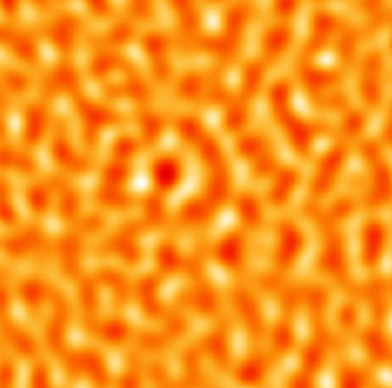
Figure 3: 16.5 GHz CAT image of $6\nobreak^{\circ}\times 6\nobreak^{\circ}$ area centred on the CAT2 field, after discrete sources have been subtracted. Excess power can be seen in the central $2\nobreak^{\circ}\times 2\nobreak^{\circ}$ primary beam (because the sensitivity drops sharply outside this area, the outer regions are a good indicator of the noise level on the map). The flux density range scale spans $\pm 40$ mJy per beam.

When interpreting this map, however, it should remembered that for an interferometer with just three horns, the ‘synthesised’ beam of the telescope has large sidelobes, and it is these sidelobes that cause the regular features seen in the map. In the full analysis of the data, these sidelobes must be carefully taken into account.

For an interferometer, ‘visibility space’ correlates directly with the space of spherical harmonic coefficients $\ell$ discussed earlier, and the data may be used to place constraints directly on the CMB power spectrum in two independent bins in $\ell$. These constraints, along with those from the other experiments, are shown in Figure 4.

Figure 4: CMB data points and the best fit power spectrum from fitting jointly with IRAS 1.2 Jy data, taken from Webster et al. [Webster et al. 1998]. The COBE data point is the 4-year COBE DMR result from Bennett et al. [Bennett et al. 1996].

g Owens Valley Radio Observatory

The Owens Valley Radio Observatory (OVRO) telescopes have been used since 1993 for observation of the CMB at $14.5~{}{\rm GHz}$ and $32~{}{\rm GHz}$. The RING40M experiment uses the 40-meter telescope ($14.5~{}{\rm GHz}$ channel) while the RING5M experiment is mounted on the 5.5-meter telescope ($32~{}{\rm GHz}$ channel). Both experiments have an angular resolution of $\sim 0.12^{\circ}$. Details about these experiments can be found in Readhead et al. [Readhead et al. 1989] or in Myers et al. [Myers et al. 1993] for example.

36 fields at Dec+$88^{\circ}$, each separated by 22 arcmin, have been observed around the North Galactic Pole. Using these data, Leitch et al. [Leitch et al. 1997] report an anomalous component of Galactic emission. Further work on the same data which has just become available [Leitch et al. 1998], gives the following estimate for the CMB component: $\mathchar 28942\relax T=56^{+8.5}_{-6.6}~{}\mathchar 28950\relax\,{\rm K}$ at $l\sim 589$. As seen in Figure 4, this new OVRO result seems to agree well with the CAT estimations and therefore helps in constraining the position of the first Doppler peak.

5 Using CMB, Large Scale Structure and Supernovae data to constrain cosmological parameters

As mentioned earlier, by comparing the observed CMB power spectrum with predictions from cosmological models one can estimate cosmological parameters. This has become an area of great current interest, with many groups carrying out the analyses for a range of assumed models. [Hancock et al. 1997, Hancock et al. 1998, Lineweaver et al. 1997] (see also Bond & Jaffe, this volume). Generally speaking, the results of using CMB data alone to do this are broadly consistent with the expected range of cosmological parameters, though perhaps with a tendency for $H_{0}$ to come out rather low (assuming spatially flat models). In an independent manner, similar predictions can be achieved by comparing Large Scale Structure (LSS) surveys with cosmological models [Willick et al. 1997, Fisher & Nusser 1996, Heavens & Taylor 1995]. Recently, Webster et al. [Webster et al. 1998] have used full likelihood calculations within a specific model in order to join together CMB and LSS predictions. This approach is complementary to that of Gawiser & Silk [Gawiser & Silk 1998], who used a compilation of large scale structure and CMB data to assess the goodness of fit of a wide variety of cosmological models. Webster et al. use results from various independent CMB experiments (the compilation used is that shown in Fig. 4) together with the IRAS 1.2 Jy galaxy redshift survey and parametrise a set of spatially flat models. Because the CMB and LSS predictions are degenerate with respect to different parameters (roughly: $\Omega_{m}{\rm vs}~{}\Omega_{\Lambda}$ for CMB; $H_{0}$ and $\Omega_{m}{\rm vs}~{}b_{\rm iras}$ for LSS), the combined data likelihood analysis allows the authors to break these degeneracies, giving new parameter constraints. Note $\Omega_{m}$ is the overall matter density, satisfying $\Omega_{\rm m}+\Omega_{\Lambda}=1$.

The results of the joint analysis are given here, as being indicative of the current constraints available from the CMB data. Fig. 5 shows the final 1-dimensional probability distributions for the main cosmological parameters after marginalizing over each of the others. The constraint $\Omega_{b}h^{2}=0.024$, where $h=H_{0}/100~{}{\rm km~{}s^{-1}}$, has been assumed, close to the value expected from primordial nucleosynthesis.

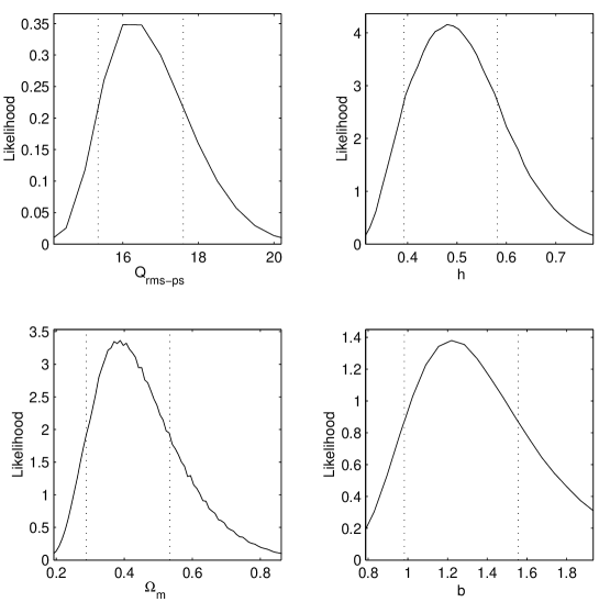
Figure 5: The one-dimensional marginalised probability distributions for each of the four parameters: $Q_{\rm rms-ps}$, the power spectrum normalization; $h=H_{0}/100~{}{\rm km~{}s^{-1}}$; $\Omega_{\rm m}$ and $b_{\rm iras}$, the (assumed linear) biasing level for IRAS galaxies. The vertical dashed lines denote the 68% confidence limits. The horizontal plot limits are at the 99% confidence limits. (Figure taken from Webster et al. [Webster et al. 1998].)

The best fit results from the joint analysis of the two data sets on all the free parameters are shown in Table 2. A detailed discussion of these estimates and comparison with other results is contained in Webster et al. [Webster et al. 1998], but in broad terms it is clear that fairly sensible values have resulted, which is encouraging for future prospects within this area.

	Free parameters
$\Omega_{\rm m}$	$0.39$	$0$.	$29$ $\,<\,$	$\Omega_{\rm m}$ $\,<\,$	$0$.	$53$
$h$	$0.53$	$0$.	$39$ $\,<\,$	$h$ $\,<\,$	$0$.	$58$
$Q$ ($\mathchar 28950\relax$K)	$16.95$	$15$.	$34$ $\,<\,$	$Q$ $\,<\,$	$17$.	$60$
$b_{\rm iras}$	$1.21$	$0$.	$98$ $\,<\,$	$b_{\rm iras}$ $\,<\,$	$1$.	$56$
	Derived parameters
$\Omega_{b}$	$0.085$
$\mathchar 28955\relax_{8}$	$0.67$
$\mathchar 28955\relax_{8,{\rm iras}}$	$0.81$
$\Gamma$	$0.15$
$\mathchar 28940\relax_{\rm iras}$	$0.47$
Age (Gyr)	$16.5$

Table 2: Parameter values at the joint optimum. For the free parameters the 68% confidence limits are shown, calculated for each parameter by marginalising the likelihood over the other variables. (Table taken from Webster et al. [Webster et al. 1998].)

For a spatially flat model, the age of the universe is given by:

$$t=\frac{2}{3H_{0}}\frac{\tanh^{-1}\sqrt{\Omega_{\Lambda}}}{\sqrt{\Omega_{\Lambda}}}$$

which evaluates to 16.5 Gyr in the current case, again compatible with previous estimates.

a Combining CMB and Supernovae data

There has recently been great interest in combining Type Ia supernovae (SN) data with results from the CMB (e.g. Tegmark et al. [Tegmark et al. 1998], Lineweaver [Lineweaver 1998]). It is instructive to see how the complementarity between the supernovae and CMB data comes about. The key quantity for this discussion from both the CMB and SN points of view is $R_{0}S(\mathchar 28959\relax)$, which occurs in the definitions of Luminosity Distance:

$$d_{L}=R_{0}S(\mathchar 28959\relax)(1+z),$$

and Angular Diameter Distance:

$$d_{\mathchar 28946\relax}=R_{0}S(\mathchar 28959\relax)/(1+z)$$

Here $\mathchar 28959\relax$ is a comoving coordinate, and $S(\mathchar 28959\relax)$ is $\sinh(\mathchar 28959\relax)$, $\mathchar 28959\relax$ or $\sin(\mathchar 28959\relax)$ depending on whether the universe is open, flat or closed respectively. For a general Friedmann-Lemaitre model, one finds that

$$R_{0}S(\mathchar 28959\relax)\propto\frac{1}{|\Omega_{\rm k}|^{1/2}}{\rm sin(h)}\left\{|\Omega_{\rm k}|^{1/2}\int_{0}^{z}\frac{dz^{\prime}}{H(z^{\prime})}\right\}$$

where

$$\Omega_{\rm k} = 1-(\Omega_{\rm m}+\Omega_{\Lambda}),$$

$$H^{2}(z) = H_{0}^{2}\left((1+\Omega_{\rm m}z)(1+z)^{2}-\Omega_{\Lambda}z(2+z)\right).$$

For small $z$, it is easy to show that

$$d_{L}\propto z+\frac{1}{2}(1-2q_{0})z^{2},$$

where $q_{0}=\frac{1}{2}(\Omega_{\rm m}-2\Omega_{\Lambda})$ is the usual deceleration parameter.

Therefore, for small $z$, SN results are degenerate along a line of constant $q_{0}$. However, the contours of equal $R_{0}S(\mathchar 28959\relax)$ shift around as $z$ increases and for $z\mbox{$\stackrel{{\scriptstyle>}}{{{}_{\sim}}}$}100$, the contours are approximately orthogonal to those corresponding to $q_{0}$ constant. This is the essence of why CMB and SN results are ideally complementary. The current microwave background data is mainly significant in delimiting the left/right position of the first Doppler peak in the power spectrum, and this depends on the cosmology via the angular diameter distance formula, evaluated at $z\sim 1000$. Thus the CMB results will tend to be degenerate along lines roughly perpendicular to those for the supernovae in the $(\Omega_{\rm m},\Omega_{\Lambda})$ plane. Detailed likelihood calculations using both supernovae and CMB data are currently being carried out by Efstathiou et al., and should be submitted shortly.

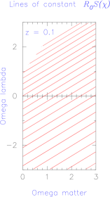
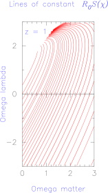
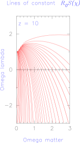
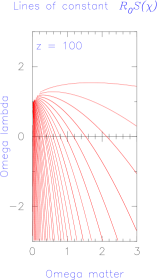
Figure 6: Plots showing contours of constant $R_{0}S(\mathchar 28959\relax)$ at redshifts of 0.1, 1, 10 and 100.

6 Future Experiments

a Ground Based Interferometers

Table 3: Future Ground Based Experiments

Experiment	Frequency	Angular Scale	Site/Type	Date
VSA	26 to 36 GHz	$0.25^{\circ}-2^{\circ}$	Tenerife (14 element interferometer)	1999
CBI	26 to 36 GHz	$0.07^{\circ}-0.3^{\circ}$	Chile (13 element interferometer)	1999
DASI	26 to 36 GHz	$0.25^{\circ}-1.4^{\circ}$	South Pole (13 element interferometer)	1999

As seen in Section 3b, interferometers allow accurate removal of the atmospheric component. Therefore special ground sites are not always necessary in order to perform sensitive measurements, as already seen for the 3 element Cosmic Anisotropy Telescope (CAT) currently operating in Cambridge, UK (see above).

The Very Small Array (VSA) is currently being built and tested in Cambridge for siting in Tenerife and should be observing in late 1999. The 14 elements of the interferometer will operate from 26 to 36 GHz and cover angular scales from $0.25^{\circ}$ to $2^{\circ}$ (see Table 3). The results will consist of 9 independent bins regularly spaced from $l\sim 150$ to $l\sim 900$ on the Power Spectrum diagram [Jones 1997]. This will give significant information on the second Doppler peak, while (subject to constraints on one of $\Omega_{\rm k}$ or $\Omega_{\Lambda}$) the first peak will be constrained accurately enough to estimate the total density $\Omega$ and Hubble’s constant $H_{0}$, with a 10% error, by the end of the year 2000. An artists impression of the VSA is shown in Fig. 7.

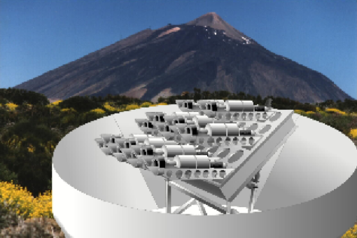
Figure 7: Artist’s impression of the VSA in operation near Mt. Teide in Tenerife.

There are two other interferometer projects which will complement the work done with the VSA: The Cosmic Background Imager (CBI), to be operated from Chile by a CalTech team [Pearson 1998] and The Degree Angular Scale Interferometer [White et al. 1997, Stark et al. 1998] (DASI) – formerly Very Compact Array (VCA) – which will be operated at the South Pole (University of Chicago & CARA). They both share the same design (13 element interferometers) and the same correlator operating from 26 to 36 GHz (see Table 3). However the size of the baselines differ between CBI and DASI so that CBI will cover angular scales from 4 to 20 arcmin while DASI will cover the range between 15 arcmin and $1.4^{\circ}$ (similar to the VSA).

All three of these interferometric experiments (VSA, CBI and DASI) should be in operation by the end of 1999.

b Forthcoming balloon experiments

The paper by Bond & Jaffe (this volume) provides details of the expected parameter-estimation performance of several upcoming balloon experiments. Here we comment briefly on the experimental aspects of the new generation of balloons.

Experiments such as MAX (e.g. Tanaka et al. [Tanaka et al. 1996]) and MSAM (e.g. Cheng et al. [Cheng et al. 1997]) have been very significant in providing CMB anisotropy data points at mm and sub-mm frequencies, and figure prominently in compilations of current data. In order to reduce the quite large scatter associated with the balloon data, however, the key requirement has been to increase the effective observing time from the 9 to 12 hours of a typical launch, so that larger sky areas can be surveyed (reducing sample variance) to greater depth. Two main ways have evolved to achieve this. The first is the use of array receivers. Here, instead of one pixel on the sky at each frequency, many are used, speeding up throughput. The MAXIMA experiment, which has grown out of the MAX program, has 8 simultaneous 12 arcmin pixels available, and has recently completed its first flight. Data from this is currently being analysed.

The second method is to directly increase the time for which the balloon can take data. This is being achieved by launching the balloons in Antarctica and relying on the circulating winds near the South Pole to sweep the balloon around in a roughly circular orbit back to the launch site, where it can be recovered. Three groups have now got funding for such experiments. These are (a) BOOMERANG (Caltech and Berkeley) in LD (Long Duration) mode, which will circle the pole in 7 to 14 days. (A preliminary flight of BOOMERANG in North America has already been completed and data is expected from this soon); (b) ACE (collaboration between UCSB, Milan and Bologna), which unlike other balloon systems uses heterodyne rather than bolometer technology (and correspondingly lower frequencies). This experiment is planned to ultimately evolve to an ultralong duration system called BEAST, which would circle the pole in about 100 days; (c) TOPHAT (collaboration between GSFC, Chicago and Barthol), which is also long duration but distinguished from BOOMERANG in that the payload is mounted on top of the balloon in an attempt to provide a more systematic-free environment. Further details of all these missions can be found in the web pages cited in the references of Bond & Jaffe (this volume).

c Satellite experiments

Two new satellite experiments to study the CMB have recently been selected as future missions. These are MAP, or Microwave Anisotropy Probe, which has been selected by NASA as a Midex mission, for launch in late 2000, and the Planck Surveyor, which has been selected by ESA as an M3 mission, and will be launched by 2007. An artist’s impression of the MAP satellite, which has five frequency channels from 30 GHz to 100 GHz, with best resolution 12 arcmin, is shown in Figure 8.

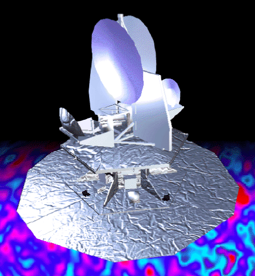
Figure 8: Artist’s impression of the MAP Satellite.

An artist’s impression of the Planck Surveyor satellite, which combines both HEMT and bolometer technology in 10 frequency channels covering the range 30 GHz to 850 GHz, with best resolution 4 arcmin, is shown in Figure 9.

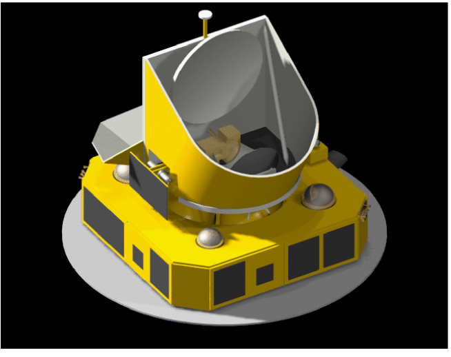
Figure 9: Artist’s impression of the Planck Surveyor Satellite (formally COBRAS/SAMBA)

Both these missions are of course of huge importance for CMB research and cosmology, and even well ahead of launch have sparked off intense theoretical interest, and many new research programmes in theoretical CMB astronomy and data analysis. There is no space here to give an adequate coverage of these missions, or the likely quality of science which will result. We content ourselves with a single illustration (Fig. 10 — taken from the Planck Phase A study), which shows the accuracy with which three of the main cosmological parameters could be recovered, as a function of resolution, if 1/3 of the sky was measured to an accuracy of $\Delta T/T=2\times 10^{-6}$ per pixel. (Note a zero cosmological constant was assumed in producing this figure.) Obviously such accuracy requires good subtraction of contaminating foregrounds and point sources, but recent advances in data analysis, particularly involving application of the maximum entropy method [Hobson et al. 1998], suggest that such accuracy is feasible.

Figure 10: Expected capability of a satellite experiment as a function of resolution. The percentage error in recovering cosmological parameters from the CMB power spectrum is shown versus the resolution available. This figure is taken from Bersanelli et al. [Bersanelli et al. 1996].

d New UK instruments proposed

In the context of a discussion meeting in the UK it is of interest to look briefly at two ground-based CMB instruments proposed by UK groups. Funding is currently being sought for each of these, which perform complementary observations, of CMB polarization, and secondary effects in the power spectrum.

i AMI — the Arc Minute Imager

This instrument is currently being proposed by MRAO, Cambridge as a follow-up to the VSA and CAT. It will be a 15 horn interferometer for CMB structure mapping on angular scales from 0.5 to 5 arcmin. It primary use will be to carry out a survey for protoclusters via the Sunyaev-Zeldovich (SZ) effect [Sunyaev & Zel’dovich 1972]. Two possible candidate high redshift clusters may already have been identified via this technique [Jones et al. 1997, Richards et al. 1997]. The number of such clusters expected is strongly cosmology dependent (e.g. Eke et al. [Eke et al. 1996]) and therefore very useful to measure, and will provide information complementary to that provided by high-redshift optical surveys. In particular, a crucial feature of the SZ effect is that (for the same cluster parameters etc.) the observed microwave decrement is independent of distance. It thus provides a very sensitive indicator of both cosmological model and cluster gas evolution properties at high redshift.

Further cosmological uses for AMI include detection of other secondary anisotropies in the power spectrum at high $\ell$’s, (e.g. the Ostriker-Vishniac effect [Ostriker & Vishniac 1986]), and imaging of the Kaiser-Stebbins effect in cosmic strings (should a string exist in the field of view), which as discussed above requires high angular resolution in order to see the non-Gaussian step-like discontinuity at the string itself.

ii CMBpol — CMB polarization experiment

This experiment, being proposed by a collaboration headed by Walter Gear of MSSL, is a ground-based instrument for measuring the CMB polarization power spectrum in the intermediate to small angular scale range. Specifically the aim is to measure about 10 to 20 square degrees of sky to an accuracy of $\sim 1\,\mathchar 28950\relax{\rm K}$ at a resolution of 3 arcmin over a period of 2 years. The instrument will use bolometric array and be mounted in Hawaii. Operation could begin in 2001–2002 if the experiment is funded.

A key experimental feature of CMB polarization is that the atmosphere itself is not polarized, and also that the polarization of a specific spot in the sky can be measured by difference measurements at that single spot. Thus the techniques discussed above in Section 3b for eliminating atmospheric noise, can be used without any beam-switching, through the same atmospheric column. This is what will allow such a sensitive measurement of polarization to be made from the ground, rather than having to be made from a satellite. Of course the total intensity component is not simultaneously available, and only a restricted range of $\ell$’s will be measured in polarization, due to the finite size of the sky patch. However, the experiment should provide the first measurement of the expected sequence of peaks in the polarization power spectrum (see Fig. 2), and provide very exciting complementary information to that which will be available from the VSA, MAP and balloon experiments by that time.

7 Conclusion

CMB experiments are already providing significant constraints on cosmological models, and future experiments will sharpen these up considerably. Although full-sky high resolution satellite experiments like Planck Surveyor will eventually provide definitive answers for the CMB, the ability of ground-based experiments and long-duration balloons to go deep on selected patches, promises to provide very interesting information within the next two years, followed shortly by the first results from MAP. Combined with data from large scale structure, supernovae distances, cluster abundances and other indicators, the next few years promise to be extremely interesting for cosmology!

References

- Baker 1997 Baker J., 1997, Imaging CMB anisotropies with CAT, in Batley R., Jones M., Green D., eds, Proceedings of the ‘Particle Physics and Early Universe Conference’, Cambridge. http://www.mrao.cam.ac.uk/ppeuc/astronomy/papers/
- Bennett et al. 1996 Bennett C. L., Banday A. J., Gorski K. M., Hinshaw G., Jackson P., Keegstra P., Kogut A., Smoot G. F., Wilkinson D. T., Wright E. L., 1996, Astrophys. J., 464, L1
- Bersanelli et al. 1996 Bersanelli M., et al., 1996, COBRAS/SAMBA report on Phase A study, in ESA document D/SCI(96)3
- Bunn et al. 1996 Bunn E., Hoffman Y., Silk J., 1996, Astrophys. J., 464, 1
- Cheng et al. 1997 Cheng E., Cottingham D., Fixsen D., Goldin A., Inman C., Knox L., Kowitt M., Meyer S., Puchalla J., Ruhl J., Silverberg R. F., 1997, Astrophys. J., 488, L59
- Coble et al. 1998 Coble K., et al., 1998, BAAS, 192, 52
- Davies et al. 1996 Davies R., Gutierrez C., Hopkins J., Melhuish S., Watson R., Hoyland R., Rebolo R., Lasenby A., Hancock S., 1996, Mon.Not.R.astr.Soc., 278, 883
- Dragovan et al. 1994 Dragovan M., Ruhl J., Novak G., Platt S., Crone B., Pernic R., Peterson J., 1994, Astrophys. J., 427, L67
- Efstathiou & Bond 1998 Efstathiou G., Bond J. R., 1998, Submitted to Mon.Not.R.astr.Soc, astro-ph/9807103
- Eke et al. 1996 Eke V., Cole S., Frenck C., 1996, Mon.Not.R.astr.Soc, 282, 263
- Femenia et al. 1998 Femenia B., Rebolo R., Gutiérrez C., Limon M., Piccirillo L., 1998, Astrophys. J., 498, 117
- Ferreira et al. 1998 Ferreira P., Magueijo J., Gorski K., 1998, Astrophys. J. (in press), astro-ph/9803256
- Fisher & Nusser 1996 Fisher K., Nusser A., 1996, Mon.Not.R.astr.Soc., 279, L1
- Gawiser & Silk 1998 Gawiser E., Silk J., 1998, Science, 280, 1405
- Gutiérrez 1997 Gutiérrez C., 1997, Astrophys. J, 483, 51
- Gutierrez et al. 1997 Gutierrez C., Hancock S., Davies R., Rebolo R., Watson R., Hoyland R., Lasenby A., Jones A., 1997, Astrophys.J.Lett., 480, L83
- Hancock et al. 1994 Hancock S., Davies R., Lasenby A., Gutierrez C., Watson R., Rebolo R., Beckman J., 1994, Nature, 367, 333
- Hancock et al. 1997 Hancock S., Gutierrez C., Davies R., Lasenby A., Rocha G., Rebolo R., Watson R., Tegmark M., 1997, Mon.Not.R.astr.Soc., 289, 505
- Hancock et al. 1995 Hancock S., Lasenby A., Gutierrez C., Davies R., Watson R., Rebolo R., 1995, Astrophys.Lett.Comm., 32, 201
- Hancock et al. 1998 Hancock S., Rocha G., Lasenby A., Gutierrez C., 1998, Mon.Not.R.astr.Soc., 294, L1
- Haslam et al. 1982 Haslam C., Salter C., Stoffel H., Wilson W., 1982, Astr. Astrophys. Suppl., 47, 1
- Heavens & Taylor 1995 Heavens A., Taylor A., 1995, Mon.Not.R.astr.Soc., 275, 483
- Herbig 1998 Herbig T., 1998, http://tyger.princeton.edu/th/mat/mat.html
- Hobson et al. 1998 Hobson M., Jones A., Lasenby A., Bouchet F., 1998, Component separation methods for satellite observations of the cosmic microwave background, To appear in Mon.Not.R.astr.Soc., astro-ph/9806387
- Jones et al. 1998 Jones A., Hancock S., Lasenby A., Davies R., Gutierrez C., Rocha G., Watson R., Rebolo R., 1998, Mon.Not.R.astr.Soc., 294(4), 582
- Jones 1997 Jones M., 1997, in Bouchet F., Gispert R., Guiderdoni B., Van J. T. T., eds, ‘Microwave Background Anisotropies’, Proceedings of the XVIth Moriond Astrophysics Meeting. Editions Frontières, p. 161
- Jones et al. 1997 Jones M., Saunders R., Baker J., Cotter G., Edge A., Grainge K., Haynes T., Lasenby A., Pooley G., Rottgering H., 1997, Astrophys.J.Lett., 479, L1
- Kaiser & Stebbins 1984 Kaiser N., Stebbins A., 1984, Nature, 310, 391
- Kovac et al. 1997 Kovac J., Dragovan M., Schleuning D., Alvarez D., Peterson J., Miller K., Platt S., Novak G., 1997, BAAS, 191, 112
- Lasenby et al. 1995 Lasenby A., Hancock S., Gutierrez C., Davies R., Watson R., Rebolo R., 1995, Astrophys.Lett.Comm., 32, 191
- Leitch et al. 1997 Leitch E., Readhead A., Pearson T., Myers S., 1997, Astrophys. J., 486, L23
- Leitch et al. 1998 Leitch E., Readhead A., T.J.Pearson Myers S., Gulkis S., 1998, Submitted to Astrophys.J., astro-ph/9807312
- Lineweaver 1998 Lineweaver C., 1998, Astrophys.J., in press, astro-ph/9805326
- Lineweaver et al. 1997 Lineweaver C., Barbosa D., Blanchard A., Bartlett J., 1997, Astron.Astrophys., 322(365)
- Lineweaver et al. 1995 Lineweaver C., Hancock S., Smoot G., Lasenby A., Davies R., Banday A., Gutierrez C., Watson R., Rebolo R., 1995, Astrophys.J., 448, 482
- Lyth & Riotto 1998 Lyth D., Riotto A., 1998, Phys.Rep., in press, hep-ph/9807278
- Magueijo & Lewin 1997 Magueijo J., Lewin A., 1997, Contribution to the proceedings of “Topological defects and CMB”, Rome, October 96, astro-ph/9702131
- Myers et al. 1993 Myers S., Readhead A., Lawrence C., 1993, Astrophys. J., 405, 8
- Netterfield et al. 1997 Netterfield C., Devlin M., Jarosik N., Page L., Wollack E., 1997, Astrophys. J., 474, 47
- Oliveira-Costa et al. 1997 Oliveira-Costa A., Kogut A., Devlin M., Netterfield C., Page L., Wollack E., 1997, Astrophys. J., 482, L17
- Ostriker & Vishniac 1986 Ostriker J., Vishniac E., 1986, Astrophys. J., 306, L51
- O’Sullivan et al. 1995 O’Sullivan C., Yassin G., Woan G., Scott P., Saunders R., Robson M., Pooley G., Lasenby A., Kenderdine S., Jones M., Hobson M., Duffett-Smith P., 1995, Mon.Not.R.astr.Soc., 274, 861
- Pearson 1998 Pearson T., 1998, http://astro.caltech.edu/tjp/CBI/
- Piccirillo 1991 Piccirillo L., 1991, Rev. Sci. Instr., 62, 1293
- Piccirillo & Calisse 1993 Piccirillo L., Calisse P., 1993, Astrophys. J., 411, 529
- Piccirillo et al. 1997 Piccirillo L., et al., 1997, Astrophys. J., 475, L77
- Platt et al. 1997 Platt S., Kovac J., Dragovan M., Nguyen H., Tucker G., 1997, Astrophys. J., 475, L1
- Readhead et al. 1989 Readhead A., Lawrence C., Myers S., Sargent W., Hardebeck H., Moffet A., 1989, Astrophys. J., 346, 566
- Richards et al. 1997 Richards E., Fomalont E., Kellermann K., Partridge R., Windhorst R., 1997, Astronom. J., 113, 1475
- Robson et al. 1993 Robson M., Yassin G., Woan G., Wilson D., Scott P., Lasenby A., Kenderdine S., Duffett-Smith P., 1993, Astron.Astr., 277, 314
- Ruhl et al. 1995 Ruhl J., Dragovan M., Platt S., Kovac J., Novak G., 1995, Astrophys. J., 453, L1
- Scott et al. 1996 Scott P., Saunders R., Pooley G., O’Sullivan C., Lasenby A., Jones M., Hobson M., Duffett-Smith P., Baker J., 1996, Astrophys.J.Lett., 461, L1
- Silk 1968 Silk J., 1968, Astrophys. J., 151, 459
- Stark et al. 1998 Stark A., Carlstrom J., Israel F., Menten K., Peterson J., Phillips T., Sironi G., Walker C., 1998, pre-print, astro-ph/9802326
- Sunyaev & Zel’dovich 1972 Sunyaev R., Zel’dovich Y. B., 1972, Comm. Astrophys. Sp. Phys., 4, 173
- Tanaka et al. 1996 Tanaka S., et al., 1996, Astrophys. J., 468, L81
- Tegmark et al. 1998 Tegmark M., Eisenstein D., Hu W., Kron R., 1998, Submitted to Astrophys. J., astro-ph/9805117
- Tegmark et al. 1997 Tegmark M., Oliveira-Costa A., Devlin M., Netterfield C., Page L., Wollack E., 1997, Astrophys. J., 474, L77
- Webster et al. 1998 Webster M., Bridle S., Hobson M., Lasenby A., Lahav O., Rocha G., 1998, Joint estimation of cosmological parameters from CMB and IRAS data, Submitted to Astrophys.J., astro-ph/9802109
- White et al. 1997 White M., Carlstrom J., Dragovan M., 1997, Submitted to Astrophys.J., astro-ph/9712195
- Willick et al. 1997 Willick J., Strauss M., Dekel A., Kolatt T., 1997, Astrophys. J., 486, 629
- Wollack et al. 1996 Wollack E., Devlin M., Jaroski N., Netterfield C., Page L., Wilkinson D., 1996, Tech. Rep. Princ. Univ, 01/1996
- Wollack et al. 1997 Wollack E., Devlin M., Jaroski N., Netterfield C., Page L., Wilkinson D., 1997, Astrophys. J., 476, 440
- Wollack et al. 1993 Wollack E., Jarosik C., Netterfield B., Page L., Wilkinson D., 1993, Astrophys. J., 419, L49
- Zaldarriaga et al. 1997 Zaldarriaga M., Spergel D., Seljak U., 1997, Astrophys. J., 488, 1