Biased-estimations of the Variance and Skewness

Abstract

Nonlinear combinations of direct observables are often used to estimate quantities of theoretical interest. Without sufficient caution, this could lead to biased estimations. An example of great interest is the skewness $S_{3}$ of the galaxy distribution, defined as the ratio of the third moment $\overline{\xi}_{3}$ and the variance squared $\overline{\xi}_{2}^{2}$ smoothed at some scale $R$. Suppose one is given unbiased estimators for $\overline{\xi}_{3}$ and $\overline{\xi}_{2}^{2}$ respectively, taking a ratio of the two does not necessarily result in an unbiased estimator of $S_{3}$. Exactly such an estimation-bias (distinguished from the galaxy-bias) affects most existing measurements of $S_{3}$ from galaxy surveys. Furthermore, common estimators for $\overline{\xi}_{3}$ and $\overline{\xi}_{2}$ suffer also from this kind of estimation-bias themselves, because of a division by the estimated mean counts-in-cells. In the case of $\overline{\xi}_{2}$, the bias is equivalent to what is commonly known as the integral constraint. We present a unifying treatment allowing all these estimation-biases to be calculated analytically. These estimation-biases are in general negative, and decrease in significance as the survey volume increases, for a given smoothing scale. We present a preliminary re-analysis of some existing measurements of the variance and skewness (from the APM, CfA, SSRS, IRAS) and show that most of the well-known systematic discrepancies between surveys with similar selection criteria, but different sizes, can be attributed to the volume-dependent estimation-biases. This affects the inference of the galaxy-bias(es) from these surveys. Our methodology can be adapted to measurements of the variance and skewness of, for instance, the transmission distribution in quasar spectra and the convergence distribution in weak-lensing maps. We discuss generalizations to $N>3$, suggest methods to reduce the estimation-bias, and point out other examples in large scale structure studies which might suffer from this type of a nonlinear-estimation-bias.

1 Introduction

There has been a long history of interests, since the pioneering work of Peebles (Peebles (1980), §18) in the hierarchical amplitudes $S_{N}$, defined as the following ratio:

$$S_{N}=\overline{\xi}_{N}/\overline{\xi}_{2}^{N-1}\,,$$ (1)

where $\overline{\xi}_{N}$ is the N-cumulant defined by $\langle\delta^{N}\rangle_{c}$, and $\delta$ is the density fluctuation smoothed on some scale. These quantities are important as a test of the gravitational instability paradigm (e.g. Fry (1984); Juszkiewicz et al. (1993); Bernardeau (1994)), a probe of possibly non-Gaussian initial conditions (e.g. Silk & Juszkiewicz (1991); Gaztañaga & Maehoenen (1996); Gaztañaga & Fosalba (1997)) as well as a measure of the galaxy-bias (e.g. Fry & Gaztañaga (1993); Frieman & Gaztañaga (1994)). However, it has also been a puzzle for quite some time that different galaxy surveys yield discordant values for $S_{N}$ (e.g. Table 1, for $N=3,4$). While some of the differences no doubt arise from the fact that galaxies selected in different ways might have different galaxy-biases, not all of the differences can be convincingly explained away in such a manner. For instance, a comparison between optically selected galaxy-catalogs (in Table 1) reveal a substantial and systematic difference between the measured values of $S_{N}$: redshift surveys consistently yield lower values compared to the larger angular catalogues (e.g. compare APM/LICK/EDSGC values with those from CfA/SSRS in Table 1; note that the IRAS galaxies are infrared-selected; note also an exception to this rule in the measurements by Kim & Strauss (1998)). A rather large relative galaxy-bias between these two sets of catalogues would have to be invoked to reconcile them.

Three alternative explanations are possible. The first is that redshift space distortions tend to suppress $S_{N}$, but it has been shown to be not sufficient to explain the systematic differences, especially on large scales (Fry & Gaztañaga (1994)). The second is that the local volume (sampled by the redshift surveys) just happens to have a smaller $S_{N}$ compared to the true $S_{N}$ which is presumably measured in the larger angular surveys i.e. the local universe is not a fair sample (e.g. Gaztañaga (1994)). This is related to the question of the homogeneity scale of our universe which has been a subject of some debate (see e.g. Wu et al. (1998) ). The third is to blame it on the estimator for $S_{N}$: it yields a value that is on the average biased low, with the bias (distinguish this from the galaxy-bias) getting worse as the survey becomes smaller. We will demonstrate that the third contributes to a significant fraction of the systematic differences between the different measurements. While a thorough analysis detailing exactly how much each of these factors contribute is beyond the scope of this paper, we can safely conclude that inference of large sampling fluctuations, or a large relative galaxy-bias, based on measurements of $S_{3}$, are unwarranted.

A very closely related estimation-bias has been discussed before by Colombi et al. (Colombi et al. (1994)) as a finite-volume effect. They attributed this to the abrupt cut-off of the count probability at some finite number of particles because of the finite size of a survey. They proposed a way to correct for this bias by extending the tail of the count probability using a few phenomenological parameters calibrated from simulations (see also Fry & Gaztañaga (1994); Munshi et al. (1997)). The method works reasonably well for small smoothing scales, but not for large ones, mainly because the probability-distribution-tail becomes noisy in the latter case (Colombi 1998, private communication). Moreover, the method is feasible only with a dense-sampled survey (Bouchet et al. (1993)). More recently, Szapudi & Colombi (Szapudi & Colombi (1996)) and Colombi et al. Colombi et al. (1998) discussed how a finite survey-volume affects the errors (i.e. the variance around the mean) in the estimators of the N-cumulants $\overline{\xi}_{N}$ (or the related factorial moments), but not the mean or bias of the estimator for $S_{N}$.

However, there has been no attempt to explain quantitatively the differences in the measured $S_{N}$ from different surveys of similar selection criteria in terms of the finite-volume effect. This is, perhaps, in part due to the lack of an analytical estimate of the systematic bias of the standard estimators for $S_{N}$. As we will show, a remarkably simple statistical fact allows just such a calculation to be done, while clarifying the origin of this bias, and relating it to other known biases in large scale structure statistics, such as the integral constraint.

Consider the following elementary statement:

$$\langle{\hat{A}\over\hat{B}}\rangle\neq{\langle\hat{A}\rangle\over{\langle\hat{B}\rangle}}$$ (2)

where $\langle\,\rangle$ denotes ensemble averaging, and $\hat{A}$ and $\hat{B}$ are two random variables or estimators. This statement holds generically, except in special cases such as when $\hat{A}$ and $\hat{B}$ are constants.

The standard method of estimating $S_{N}$ is to form estimates of $\overline{\xi}_{N}$ and $\overline{\xi}_{2}$ separately, and then take an appropriate ratio of the two. However, even in the ideal case where one has an unbiased estimator of the numerator ($\overline{\xi}_{N}$; let us call this estimator $\hat{A}$, i.e. $\langle\hat{A}\rangle=\overline{\xi}_{N}$) and an unbiased estimator of the denominator ($\overline{\xi}_{2}^{N-1}$; let us call the estimator $\hat{B}$, i.e. $\langle\hat{B}\rangle=\overline{\xi}_{2}^{N-1}$) , taking a ratio of the two estimators does not necessarily result in an unbiased estimator of $S_{N}$. This is captured by the statistical statement in eq. (2). We will refer to this kind of estimation-bias as the ratio-bias.

More generally, nonlinear combinations of unbiased estimators should be treated with great care. For instance, suppose ${\hat{\overline{\xi}}}_{2}$ is an unbiased estimator of $\overline{\xi}_{2}$ such that $\langle{\hat{\overline{\xi}}}_{2}\rangle=\overline{\xi}_{2}$. It is virtually guaranteed that $\langle({\hat{\overline{\xi}}}_{2})^{2}\rangle\neq(\overline{\xi}_{2})^{2}$. We will refer to this kind of bias generally as a nonlinear-estimation-bias, of which the ratio-bias is a particularly simple and common example. In this paper, we will sometimes be abusing the terminology by using the two terms interchangeably.

The well-known integral constraint, in the case of measurements of the two-point function, can in fact be understood as a ratio bias. The two-point function $\xi_{2}(i,j)$, where $i$ and $j$ are two cells separated by some distance, is by definition $\langle\delta_{i}\delta_{j}\rangle$ where $\delta_{i}$ is the overdensity at cell $i$. The catch is that one directly observes only $n_{i}$, the number of particles/galaxies in a cell. An estimate of the mean number count $\bar{n}$ has to be made in order to assign a value $\delta_{i}$ for each cell. This is generally taken to be $\sum_{i}n_{i}/N_{T}$ where $N_{T}$ is the total number of cells, let us call this estimator ${\hat{\bar{n}}}$. The problem is, of course, that $\langle(n_{i}-{\hat{\bar{n}}})(n_{j}-{\hat{\bar{n}}})/{\hat{\bar{n}}}^{2}\rangle\neq\xi(i,j)$, because of the estimator $\hat{\bar{n}}$ in the denominator. As we will see, this estimation-bias is in general negative. This is what the integral constraint is about: that the measured two-point function is generally biased low because the mean number density is estimated from the same survey from which $\xi_{2}$ is being measured. This turns out to be the ratio-bias in disguise. It is also easy to see that estimates of $\xi_{N}$ would suffer from a similar bias.

Peebles Peebles (1980) first pointed out the integral-constraint-bias for estimating $\xi_{2}$, but his treatment only gave the large scale estimation-bias. Bernstein Bernstein (1994), building on earlier work by Landy & Szalay Landy & Szalay (1993), developed a perturbative approach (not perturbative in the usual sense of small density fluctuations, but perturbative in the small quantity: the average of the two-point function over the volume of the survey) to compute the full integral-constraint-bias for $\xi_{2}$, which accounted for the small-scale bias as well. (See also Kerscher (1998) for a related recent discussion.) Obviously, the integral-constraint bias affects also measurements of the one-point analogue, or the volume-average, of $\xi_{2}$ i.e. the variance $\overline{\xi}_{2}$. This integral-constraint-bias generally decreases in magnitude with increasing survey size, causing measurements of the correlation length from $\xi_{2}$ or $\overline{\xi}_{2}$ to increase with sample depth, an effect that has been observed before (Davis et al. (1988); Bouchet et al. (1993)). Hence, in the case of the two-point function or its volume average, the finite-volume-effect pointed out by Colombi et al. Colombi et al. (1994) is none other than the integral-constraint-bias.

Adopting the techniques of Bernstein Bernstein (1994), we compute analytically the biases of the standard estimators for $\overline{\xi}_{N}$ and $S_{N}$, for $N=2,3$. The methodology for a general $N$ is presented in §2. For simplicity, we illustrate how to keep track of the perturbative-ordering by going into details of the calculation for $N=2,3$. These cases are also of special interest because many measurements of $\overline{\xi}_{2}$, $\overline{\xi}_{3}$ and $S_{3}$ exist in the literature. We go over the calculation of the estimation-biases for these three quantities in §3. For readers not interested in the details: much of the section can be skipped; the main results are in eq. (27), (28) & (29).

We next check in §4 our analytical results using N-body simulations of the SCDM (Standard Cold-Dark-Matter) and LCDM (Lambda or Low-Density Cold-Dark-Matter) models. Ensemble averages of the standard estimators for $\overline{\xi}_{2}$ and $S_{3}$ are computed by using $10$ realizations for each chosen model and for various sample-volumes. The overall agreement is excellent. We also introduce a way to correct for the analytical estimates when the estimation-bias becomes so large that the perturbative approach in §3 breaks down.

In §5, we present a first step towards a re-evaluation of existing measurements of the variance and skewness from the CfA/SSRS/APM surveys. We study simulated CfA/SSRS/APM catalogues with the appropriate sizes, which include the effects of redshift distortions as well as sparse-sampling. We then consider a preliminary correction of the existing measurements of the variance and skewness from these surveys, based on our findings in §3 and §4. The correction is necessarily model-dependent (dependent on the power spectrum and the galaxy-biasing assumed), but it appears that most of the systematic differences between these surveys can be explained by the estimation-biases, under reasonable assumptions. A thorough analysis of the remaining differences would require a careful study of, among other things, projection effects and redshift distortions. We leave this for future work.

Finally, we conclude in §6 with a discussion of methods for measuring $S_{N}$ that might be subject to a less severe estimation-bias. We list other large scale structure statistics which might also suffer from this type of a nonlinear-estimation-bias. We also discuss applications of our findings outside conventional galaxy surveys, such as the Lyman-alpha forest, high-redshift Lyman-break galaxy surveys and weak-lensing maps.

2 Biases of the Standard Estimators for $\overline{\xi}_{N}$ and $S_{N}$

2.1 Definitions

The standard estimator for $S_{N}$ is given by:

$$\hat{S}_{N}=\hat{\overline{\xi}}_{N}/({\hat{\overline{\xi}}_{2}})^{N-1}\,.$$ (3)

We use $\hat{}$ to denote estimators of quantities we are interested in.

$\hat{\overline{\xi}}_{2}$ is the esimator for the variance:

$$\hat{\overline{\xi}}_{2}={1\over N_{T}}\sum_{i}(\hat{\delta}_{i})^{2}-\hat{\overline{\xi}}_{2}^{\rm shot}.$$ (4)

Imagine that the survey is divided into many very small cells, so small that the number of particles/galaxies in each cell is either 1 or 0. The index $i$ above denotes such a cell, and $N_{T}$ is the total number of such cells. $\hat{\delta}_{i}$ is an estimate of the local overdensity smoothed over some given radius $R$. We will assume top-hat smoothing in this paper. In other words:

$$\hat{\delta}_{i}=\sum_{j}{n_{j}-\hat{\bar{n}}\over\hat{\bar{n}}}W_{T}(i,j)\,,$$ (5)

where $n_{j}$ is equal to 1 if there is a galaxy and 0 otherwise, $\hat{\bar{n}}$ is an estimate of the mean density of the survey, and $W_{T}(i,j)$ is the top-hat smoothing window. The estimator $\hat{\bar{n}}$ is

$$\hat{\bar{n}}={1\over N_{T}}\sum_{i}\sum_{j}n_{j}W_{T}(i,j)\,.$$ (6)

We have not stated explicitly how to handle edge-effects. For instance, what should be done when the top-hat window $W_{T}$ overlaps with the boundary in eq. (5)? Note that $\sum_{j}W_{T}(i,j)=1$ only for $i$ sufficiently far away from edges. If one adopts the strategy that one picks only $i$’s in eq. (5) such that the top-hat does not overlap with the boundary, then the corresponding $N_{T}$ in eq. (4) should not be the total number of all infinitesimal cells in the sample, but a smaller number: the number of centers (at the infinitesimal cells) of top-hats whose windows do not overlap with the boundary. The $j$-index in eq. (5) should, on the other hand, range over the whole survey volume, up to the boundary.

The standard shot-noise correction is given by

$$\hat{\overline{\xi}}_{2}^{\rm shot}={1\over\hat{N_{R}}}$$ (7)

where $\hat{N_{R}}$ is the estimated mean number of particles within a smoothing top-hat of size $R$, in other words, it is $\hat{\bar{n}}V_{R}$ where $V_{R}$ is the volume of the top-hat.

Phrased in the above manner, the estimator $\hat{\overline{\xi}}_{2}$ is equivalent to the standard estimator for the variance using the counts-in-cells method, infinitely sampled (see Szapudi (1998)).

The estimator for the N-th cumulant is defined similarly:

$$\hat{\overline{\xi}}_{N}={1\over N_{T}}\sum_{i}(\hat{\delta}_{i})_{c}^{N}-\hat{\overline{\xi}}_{N}^{\rm shot}\,$$ (8)

where the subscript $c$ denotes the connected part of the sum, and $\hat{\overline{\xi}}_{N}^{\rm shot}$ is a shot-noise correction generalizing $\hat{\overline{\xi}}_{2}^{\rm shot}$. It is worthwhile at this point to introduce the continuum notation. We will replace $\sum_{i}/N_{T}$ by $\int dV_{i}/V_{T}$, where $dV_{i}$ is the volume of the i-th cell and $V_{T}$ is the total volume, and $W_{T}(i,j)$ by the continuum top-hat $W(i,j)$ normalized so that $\int dV_{j}\,W(i,j)=1$ for $i$ sufficiently far away from edges.

It is also worthwhile to note that factorial moments are sometimes used to estimate $\overline{\xi}_{N}$, which represents a convenient way to eliminate the shot-noise contribution (Szapudi & Szalay (1993)), but otherwise results in the same estimator for $\overline{\xi}_{N}$ as in eq. (8).

2.2 Derivation of the Estimation-Biases: an Outline

The integral-constraint-bias for $\hat{\overline{\xi}}_{2}$ arises from the fact that the true mean density $\bar{n}$ is unknown, and has to estimated from the same sample from which one tries to measure the variance. To derive it, let us first write the estimator for the mean density as $\hat{\bar{n}}=\bar{n}(1+\alpha)$, where $\hat{\bar{n}}$ is given in eq. (6), and $\alpha$ is a small fluctuation from the true mean. Then one can express the estimator for the overdensity $\hat{\delta}_{i}$ (eq. [5]) as

$$\hat{\delta}_{i}=(\delta_{i}-\alpha)(1-\alpha+\alpha^{2}-...)\,,$$ (9)

where $\delta_{i}$ is now the true overdensity (smoothed with the same top-hat as $\hat{\delta}_{i}$ is) i.e. $\delta_{i}$ is $n_{i}/\bar{n}-1$, appropriately smoothed. $\alpha$ is by definition equal to

$$\alpha={1\over V_{T}}{\int dV_{i}\delta_{i}}\,.$$ (10)

Substituting the above into the expression for $\hat{\overline{\xi}}_{2}$ (eq. [4]), one can expand in $\alpha$ and write down the ensemble average of $\hat{\overline{\xi}}_{2}$ order by order. It can be easily shown that the zero-th order term (no $\alpha$) of $\langle\hat{\overline{\xi}}_{2}\rangle$ gives $\overline{\xi}_{2}$, the true variance. The rest of the terms represent the integral-constraint-bias. A key question is by what order one should stop, which we will discuss in detail in §3.1. It suffices to note here that, strictly speaking, $\alpha$ by itself cannot be used as an ordering-parameter, because it is a random variable (depends on the data) which gets ensemble-averaged. Let us denote the integral-constraint-bias for $\hat{\overline{\xi}}_{2}$, or more generally, $\hat{\overline{\xi}}_{N}$ by:

$$\langle\hat{\overline{\xi}}_{N}\rangle\equiv\overline{\xi}_{N}(1+{\Delta_{\overline{\xi}_{N}}\over\overline{\xi}_{N}})\,.$$ (11)

As we will see, the fractional bias ${\Delta_{\overline{\xi}_{N}}/\overline{\xi}_{N}}$ becomes small for a large enough survey. This is the limit in which we will be working. How large is large, or how small is small, is the question we would like to address.

It is easy to see that the above methodology can be adopted for computing the ensemble average of the standard estimator for the hierarchical amplitude, $\langle\hat{S}_{N}\rangle$. The key idea is to assume the denominator part of the estimator fluctuates about its mean, and expand in that fluctuation. In other words, for $S_{N}$, let us first assume

$$\hat{\overline{\xi}}_{2}\equiv\overline{\xi}_{2}(1+{\Delta_{\overline{\xi}_{2}}\over\overline{\xi}_{2}})(1+\epsilon)\,,$$ (12)

where $\epsilon$ is a small fluctuation of the measured $\hat{\overline{\xi}}_{2}$ from its mean (which is offset from the true $\overline{\xi}_{2}$ by a bias; eq. [11]). Note that $\epsilon$ depends on the data, and so cannot be taken out of $\langle\rangle$.

Putting eq. (11) and (12) into eq. (3), one obtains the following expression for the mean of $\hat{S}_{N}$:

$$\langle\hat{S}_{N}\rangle = S_{N}(1+{\Delta_{S_{N}}\over S_{N}})$$ (13)

$${\Delta_{S_{N}}\over S_{N}} = {\Delta_{\overline{\xi}_{N}}\over\overline{\xi}_{N}}-(N-1){\Delta_{\overline{\xi}_{2}}\over\overline{\xi}_{2}}-(N-1){\langle\epsilon\hat{\overline{\xi}}_{N}\rangle\over\overline{\xi}_{N}}+(N-1){N\over 2}{\langle\epsilon^{2}\hat{\overline{\xi}}_{N}\rangle\over\overline{\xi}_{N}}+...\,.$$ (14)

Note that all terms up to $\epsilon^{2}$ are displayed above, except for the terms: $-(N-1)(\Delta_{\overline{\xi}_{2}}/\overline{\xi}_{2})[\langle\epsilon\hat{\overline{\xi}}_{N}\rangle/\overline{\xi}_{N}]$ and $(N-1){N\over 2}(\Delta_{\overline{\xi}_{2}}/\overline{\xi}_{2})[\langle\epsilon^{2}\hat{\overline{\xi}}_{N}\rangle/\overline{\xi}_{N}]$. As we will show later on, the terms $\Delta_{\overline{\xi}_{2}}/\overline{\xi}_{2}$, $\langle\epsilon\hat{\overline{\xi}}_{N}\rangle/\overline{\xi}_{N}$ and $\langle\epsilon^{2}\hat{\overline{\xi}}_{N}\rangle/\overline{\xi}_{N}$ are all of the order of a small parameter in which we will be expanding: hence the dropping of products involving them.

It is instructive to divide the net bias of the estimator $\hat{S}_{N}$ into two different contributions. One is due to the integral-constraint-bias discussed above: namely that both ${{\hat{\overline{\xi}}}}_{N}$ in the numerator and ${{\hat{\overline{\xi}}}}_{2}$ in the denominator (see eq. [3]) are biased estimators. This gives the first two terms on the right hand side of eq. (14). The other contribution arises from the fact that the estimator $\hat{S}_{N}$ is the ratio of two other estimators (to be accurate, it is in fact some nonlinear combinations of ${{\hat{\overline{\xi}}}}_{N}$ and ${{\hat{\overline{\xi}}}}_{2}$). This is the rest of the terms in eq. (14). Let us give these two kinds of terms explicit names:

$${\Delta_{S_{N}}^{\rm int.constr.}\over S_{N}}={\Delta_{\overline{\xi}_{N}}\over\overline{\xi}_{N}}-(N-1){\Delta_{\overline{\xi}_{2}}\over\overline{\xi}_{2}}\,,$$ (15)

$${\Delta_{S_{N}}^{\rm ratio}\over S_{N}}=-(N-1){\langle\epsilon\hat{\overline{\xi}}_{N}\rangle\over\overline{\xi}_{N}}+(N-1){N\over 2}{\langle\epsilon^{2}\hat{\overline{\xi}}_{N}\rangle\over\overline{\xi}_{N}}\,,$$ (16)

the integral-constraint-bias and the ratio-bias of $\hat{S}_{N}$ respectively. We are slightly abusing the terminology here because the integral-constraint-bias is of course itself a form of a ratio-bias. As we will show below, it turns out that the terms contributing to the integral-constraint-bias partially cancel each other, leaving the ratio-bias to be the dominant contribution to the net bias of $\hat{S}_{N}$ on large scales.

Note that we have implicitly assumed ${\Delta_{\overline{\xi}_{N}}/\overline{\xi}_{N}}$, $(N-1){\Delta_{\overline{\xi}_{2}}/\overline{\xi}_{2}}$ and $(N-1){\langle\hat{\overline{\xi}}_{N}\epsilon\rangle/\overline{\xi}_{N}}$ and $(N-1)N\langle\epsilon^{2}\hat{\overline{\xi}}_{N}\rangle/2\overline{\xi}_{N}$ are all small, and that terms we have ignored in eq. (14) are somehow all of higher order. What is the correct ordering parameter in which we are expanding? Again, the quantity $\epsilon$ cannot be used directly to keep track of the ordering, because it is data-dependent. For instance, after taking the expectation values, it could happen that terms that contain $\epsilon^{2}$ are actually comparable to terms linear in $\epsilon$. We will see that this is indeed the case in the next section.

eq. (13) implies the bias of $\hat{S}_{N}$ depends in general on the $M$-point correlation functions. The strategy we adopt in this paper is to assume the following hierarchical relation: $\xi_{M}\sim\xi_{2}^{M-1}$, which is motivated by perturbation theory but has been observed to hold in the highly nonlinear regime as well. We do not need to assume anything, however, about the configuration or scale dependence (or independence) of the hierarchical amplitudes. Using this relation, it can be shown that (we will demonstrate this explicitly for $S_{3}$) the terms we have kept in $\Delta_{S_{N}}/S_{N}$ (eq. [14]) all contain terms linear in the following quantity:

$$\overline{\xi}_{2}^{L}\equiv{1\over V_{T}^{2}}\int dV_{i}dV_{j}\xi_{2}(i,j)$$ (17)

where $\xi_{2}$ is a smoothed version of the 2-point function defined as

$$\xi_{2}(i,j)=\int dV_{k}dV_{l}\,\,\xi_{2}^{\rm usmth.}(k,l)\,W(k,i)W(l,j)$$ (18)

where $W$ is the top-hat smoothing window of some radius $R$, and $\xi_{2}^{\rm usmth.}$ is the unsmoothed 2-point function. $\overline{\xi}_{2}^{L}$ is the 2-point function averaged over the whole survey (of size $L$). For a survey to be of any use at all, this quantity has to be much smaller than 1. Because of the relatively large coefficients that will be multiplying it in $\Delta_{S_{N}}/S_{N}$, as will be shown below, the fractional bias in $\hat{S}_{N}$ could be non-negligible, even for a relatively large survey volume.

One should therefore view the derivation of the bias in $\hat{S}_{N}$ in this paper as an expansion in the small parameter $\overline{\xi}_{2}^{L}$. As we will see, the same applies to $\hat{\overline{\xi}}_{N}$. Indeed, it can be shown that all the terms we have kept in eq. (13) contain terms linear in $\overline{\xi}_{2}^{L}$, and terms we have ignored are all of higher order ($[\overline{\xi}_{2}^{L}]^{2}$, etc). We will demonstrate the reasoning with an example: $N=3$.

3 Estimation-Biases for the Variance, the Third Moment and the Skewness

3.1 The Integral-Constraint-Bias for $\hat{\overline{\xi}}_{2}$

The integral-constraint-bias for the two-point function has been known for a long time (see e.g. Peebles (1980); Bernstein (1994); Tegmark et al. (1998)). Our treatment follows most closely that of Bernstein Bernstein (1994), and the emphasis is on techniques that can be generalized to ${\hat{\overline{\xi}}}_{3}$ and $\hat{S}_{3}$.

Following the strategy outlined in §2.2, namely combining eq. (9), (10) with (4), we obtain

$$\langle\hat{\overline{\xi}}_{2}\rangle= {1\over V_{T}}\int dV_{i}\langle\delta_{i}^{2}\rangle-\langle\hat{\overline{\xi}}_{2}^{\rm shot}\rangle$$

$$-{1\over V_{T}^{2}}\int dV_{i}dV_{j}\langle\delta_{i}\delta_{j}\rangle-{2\over V_{T}^{2}}\int dV_{i}dV_{j}\langle\delta_{i}^{2}\delta_{j}\rangle$$

$$+{3\over V_{T}^{3}}\int dV_{i}dV_{j}dV_{k}\langle\delta_{i}^{2}\delta_{j}\delta_{k}\rangle+{4\over V_{T}^{3}}\int dV_{i}dV_{j}dV_{k}\langle\delta_{i}\delta_{j}\delta_{k}\rangle+...$$

where we display all terms up to $O(\alpha^{2})$ (see eq. [10]).

As we have explained before, $\alpha$ cannot really be used as an ordering-parameter, because it is a random variable which gets averaged over. The key to the above expansion is instead to keep only terms up to linear order in $\overline{\xi}_{2}^{L}$ (eq. [17]).

Ignoring shot-noise for now, the first term on the right gives us the true variance $\overline{\xi}_{2}$. This is the zero-th order term. The rest of the terms represent the integral-constraint-bias for ${\hat{\overline{\xi}}}_{2}$, and are all of order $\overline{\xi}_{2}^{L}$ or higher. Let us check.

1. The first term on the second line of eq. (3.1) is none other than $-\overline{\xi}_{2}^{L}$ itself (eq. [17]).

2. The next term, again ignoring shot-noise for now, gives $(-2/V_{T}^{2})\int dV_{i}dV_{j}\xi_{3}(i,i,j)$. Applying the hierarchical relation $\xi_{M}\sim\xi_{2}^{M-1}$, i.e. $\xi_{3}(i,i,j)\sim\xi_{2}(i,i)\xi_{2}(i,j)+...$, we can see that the term $\xi_{2}(i,i)\xi_{2}(i,j)=\bar{\xi}_{2}\xi_{2}(i,j)$, when integrated over $i$ and $j$, will give rise to a term proportional to $\xi_{2}^{L}$. Hence, the term $(-2/V_{T}^{2})\int dV_{i}dV_{j}\xi_{3}(i,i,j)$ contains a linear piece and should not be thrown away. Note that we need not make any assumption about the configuration or scale dependence of the hierarchical amplitudes. In other words, we should keep the term $(-2/V_{T}^{2})\int dV_{i}dV_{j}\xi_{3}(i,i,j)$ as is, rather than as, say $(-2/V_{T}^{2})\bar{\xi}_{2}\int dV_{i}dV_{j}\xi_{2}(i,j)$. The hierarchical relation is used strictly for keeping track of the ordering at this stage.

3. The integrand in the next term, 3 $\langle\delta_{i}^{2}\delta_{j}\delta_{k}\rangle$, can be broken up into several disconnected pieces: $3\langle\delta_{i}^{2}\delta_{j}\delta_{k}\rangle=3[\xi_{2}(i,i)\xi_{2}(j,k)+2\xi_{2}(i,j)\xi_{2}(i,k)+\xi_{4}(i,i,j,k)]$. It is easy to see that the second piece gives something that is second order in $\overline{\xi}_{2}^{L}$, when integrated over, and so does the $\xi_{4}(i,i,j,k)$ piece, assuming again the hierarchical relation. The only piece that survives is then, after integration, $3\overline{\xi}_{2}\overline{\xi}_{2}^{L}$.

4. Lastly, the $(4/V_{T}^{3})\int dV_{i}dV_{j}dV_{k}\langle\delta_{i}\delta_{j}\delta_{k}\rangle$ term in eq. (3.1) is second order in $\overline{\xi}_{2}^{L}$, again by applying the hierarchical relation.

More generally, it can be seen that all terms, including those not explicitly displayed, in the expansion in eq. (3.1) are of the form $V_{T}^{-m}\int dV_{i_{1}}...dV_{i_{m}}\langle\delta_{i_{1}}^{\gamma}\delta_{i_{2}}...\delta_{i_{m}}\rangle$, where $\gamma$ is 1 or 2. Our arguments above show that only terms with $m=1$, or $m=2$, or $m=3$ and $\gamma=2$, contain pieces linear in $\overline{\xi}_{2}^{L}$. The reader can convince himself or herself that all other terms are of higher order.

Putting everything together, ignoring shot-noise, and using the definition of the fractional bias in eq. (11), we obtain to linear order in $\overline{\xi}_{2}^{L}$,

$${\Delta_{\overline{\xi}_{2}}\over\overline{\xi}_{2}}= -{1\over\overline{\xi}_{2}V_{T}^{2}}\int dV_{i}dV_{j}\xi_{2}(i,j)-{2\over\overline{\xi}_{2}V_{T}^{2}}\int dV_{i}dV_{j}\xi_{3}(i,i,j)$$

$$+{3\over V_{T}^{2}}\int dV_{i}dV_{j}\xi_{2}(i,j)\,.$$

The above result is consistent with that of Bernstein Bernstein (1994) for the integral-constraint-bias of the two-point function. The first term on the right was obtained by Peebles Peebles (1980) via a different argument.

How about shot-noise? A term like $\langle\delta_{i}\delta_{j}\rangle$ that shows up in eq. (3.1) includes both the cosmic 2-point correlation $\xi_{2}(i,j)$ (see eq. [18]) and a shot-noise contribution due to Poisson sampling (see e.g. Feldman et al. (1994)):

$$\langle\delta_{i}\delta_{j}\rangle=\xi_{2}(i,j)+{1\over\bar{n}}\int dV_{k}W(k,i)W(k,j)$$ (21)

It can be shown that all shot-noise contributions to $\Delta_{\overline{\xi}_{2}}/\overline{\xi}_{2}$ can be expanded in either $1/N_{R}$ or $1/N_{L}$ where $N_{R}$ is the mean number of particles in a cell of size $R$, and $N_{L}$ is the mean number of particles in the whole survey. For instance, the term $V_{T}^{-1}\int dV_{i}\langle\delta_{i}^{2}\rangle$ has a Poisson term $1/N_{R}$, if one makes use of eq. (21), together with the fact that $W$ is a top-hat of size $R$ with the normalization $\int dV_{j}W(i,j)=1$. This gets canceled by part of the shot-noise correction term $-\langle{\hat{\overline{\xi}}}_{2}^{\rm shot}\rangle$ (eq. [3.1]). On the other hand, a term like $V_{T}^{-2}\int dV_{i}dV_{j}\langle\delta_{i}\delta_{j}\rangle$ gives us a Poisson term of the order of $1/N_{L}$. In general, $1/N_{L}$ is a very small quantity, and so we can ignore all terms of order $1/N_{L}$. There are, for instance, Poisson pieces linear in $\overline{\xi}_{2}^{L}$ in the $\langle\delta_{i}\delta_{j}\delta_{k}\rangle$ term in eq. (3.1), but they are also of order $1/N_{L}$, and so can be ignored.

How about the $O(1/N_{R})$ terms in eq. (3.1)? Without going into details, it can be shown that the only $O(1/N_{R})$ contributions are: $-\overline{\xi}_{2}^{L}/N_{R}$ from the $-\langle{\hat{\overline{\xi}}}_{2}^{\rm shot}\rangle$ term, $-2\overline{\xi}_{2}^{L}/N_{R}$ from the fourth term on the right, and $3\overline{\xi}_{2}^{L}/N_{R}$ from the fifth term on the right. Therefore, to $O(1/N_{R})$, the shot-noise terms miraculously cancel! It is interesting to note that this cancellation is possible only because the integral-constraint-bias in the shot-noise correction itself is taken into account i.e. $\langle{\hat{\overline{\xi}}}_{2}^{\rm shot}\rangle=\langle 1/\hat{N}_{R}\rangle=(1+\langle\alpha^{2}\rangle...)/N_{R}$ (see eq. [7] & [10]).

We will see in §4 that our estimations of the biases in the variance and skewness which ignores shot-noise are in fact quite accurate. With no further justification, we will ignore shot-noise terms in the rest of our derivation, which substantially simplifies our expressions. The cancellation to $O(1/N_{R})$ here for $\Delta_{\overline{\xi}_{2}}/\overline{\xi}_{2}$ can be taken as suggestive evidence that shot-noise is unimportant for the estimation-biases we are interested in; we will rely on the numerical simulations in §4 for further support. We should emphasize, however, we are not saying that there is no need to subtract out shot-noise when estimating the variance and skewness themselves.

Finally, how about edge-effects? It is worth emphasizing that no assumptions about the edge-effects being small need to be made in deriving eq. (3.1). One only has to be careful about volume over which the integration is done and what $V_{T}$ has to be. As we have mentioned earlier in §2.1, one way to deal with the boundary is to use only cells that do not overlap with the edges. In that case, the dummies of integration $i$ and $j$ should range over the inner part of the survey, where any cell that is centered within it does not cut into the boundary. Similarly, $V_{T}$ should be chosen to be the volume of that inner region. We will discuss how to approximate such integrals in §3.4.

3.2 The Integral-Constraint-Bias for $\hat{\overline{\xi}}_{3}$

Similarly, one can derive the integral-constraint-bias for the third cumulant using eq. (8), (11) and (9) . Ignoring shot-noise, and again, keeping only terms to first order in $\overline{\xi}_{2}^{L}$, the integral-constraint-bias for $\overline{\xi}_{3}$ is given by

$${\Delta_{\overline{\xi}_{3}}\over\overline{\xi}_{3}}= -{3\over\overline{\xi}_{3}V_{T}^{2}}\int dV_{i}dV_{j}\xi_{3}(i,i,j)-{9\overline{\xi}_{2}\over\overline{\xi}_{3}V_{T}^{2}}\int dV_{i}dV_{j}\xi_{2}(i,j)$$

$$-{3\over\overline{\xi}_{3}V_{T}^{2}}\int dV_{i}dV_{j}\xi_{4}(i,i,i,j)+{9\overline{\xi}_{2}\over\overline{\xi}_{3}V_{T}^{2}}\int dV_{j}dV_{k}\xi_{2}(j,k)$$

$$+{6\over V_{T}^{2}}\int dV_{j}dV_{k}\xi_{2}(j,k)$$

Note that by essentially the same reasoning as in the case of $\hat{\overline{\xi}}_{2}$, one only needs to consider terms up to $\alpha^{2}$ in deriving the above.

3.3 The Estimation-Bias $\hat{S}_{3}$

The integral-constraint-bias for $\hat{S}_{3}$ can be simply read off from eq. (15), (3.1) & (3.2). The ratio-bias for $\hat{S}_{3}$, on the other hand, follows from eq. (16). Substituting the definition of $\epsilon$ from eq. (12), we obtain

$${\Delta_{S_{3}}^{\rm ratio}\over S_{3}}= {-2\over\overline{\xi}_{3}\overline{\xi}_{2}(1+{\Delta_{\overline{\xi}_{2}}\over\overline{\xi}_{2}})}\langle\hat{\overline{\xi}}_{3}[\hat{\overline{\xi}}_{2}-\overline{\xi}_{2}(1+{\Delta_{\overline{\xi}_{2}}\over\overline{\xi}_{2}})]\rangle$$

$$+{3\over\overline{\xi}_{3}\overline{\xi}_{2}^{2}(1+{\Delta_{\overline{\xi}_{2}}\over\overline{\xi}_{2}})^{2}}\langle\hat{\overline{\xi}}_{3}[\hat{\overline{\xi}}_{2}-\overline{\xi}_{2}(1+{\Delta_{\overline{\xi}_{2}}\over\overline{\xi}_{2}})]^{2}\rangle\,.$$

Substituting eq. (3.1), (3.2) and (3.3) into eq. (13) for $N=3$, ignoring shot-noise terms and keeping only terms linear in $\overline{\xi}_{2}^{L}$, it can be shown that

$${\Delta_{S_{3}}^{\rm ratio}\over S_{3}}= -{6\over V_{T}^{2}\overline{\xi}_{3}}\int dV_{i}dV_{j}\xi_{3}(i,j,j)-{2\over V_{T}^{2}\overline{\xi}_{2}\overline{\xi}_{3}}\int dV_{i}dV_{j}\xi_{5}(i,i,i,j,j)$$

$$+{3\over V_{T}^{2}\overline{\xi}_{2}^{2}}\int dV_{j}dV_{k}\xi_{4}(j,j,k,k)\,,$$

where $\xi_{N}$ is the connected N-point function. The first two terms here arise from the first term on the right hand side of eq. (3.3), and the last term from the second one.

The reasoning used to arrive at the above expression is again very similar to the case of $\hat{\overline{\xi}}_{2}$. But there are a few new tips to keep in mind.

1. Consider a term like $\langle\delta_{i}^{3}[\delta_{j}^{2}-\overline{\xi}_{2}(1+\Delta_{\overline{\xi}_{2}}/\overline{\xi}_{2})]\rangle$, which arises from the first term on the right of eq. (3.3). It can be seen that a disconnected piece with the $j$ index all by itself, such as $\langle\delta_{i}^{3}\rangle\langle\delta_{j}^{2}\rangle$, is going to be canceled, by $-\langle\delta_{i}^{3}\rangle\overline{\xi}_{2}(1+\Delta_{\overline{\xi}_{2}}/\overline{\xi}_{2})$. More generally, it can be seen that all terms in the expansion of eq. (3.3) contain an integrand of the form $\langle\delta_{i}^{3}\delta_{j_{1}}^{2}\delta_{j_{2}}^{2}...\delta_{j_{m}}^{2}\rangle$, any disconnected piece of which with the $j_{1}$, or … $j_{m}$ index all by itself is going to get canceled. In other words, the $j$-indices must be connected to each other, or to $i$.

2. As before, integrals over products of the two-point function, of the form $\langle\delta_{i}\delta_{j}\rangle\langle\delta_{j}\delta_{k}\rangle$ for instance, are of higher order. An example is from the second term on the right of eq. (3.3). It contains a term with $\langle\delta_{i}^{3}\delta_{j}^{2}\delta_{k}^{2}\rangle$ in the integrand. This can be broken up into several disconnected pieces. Most of them got canceled because of the reason laid out in 1. above. One disconnected piece that does not get canceled is $\langle\delta_{i}^{3}\delta_{j}\rangle\langle\delta_{j}\delta_{k}^{2}\rangle$. However, applying the hierarchical relation as before, we can see that this piece, when integrated over, is second order in $\overline{\xi}_{2}^{L}$. Another disconnected piece is: $\langle\delta_{i}^{3}\rangle\langle\delta_{j}\delta_{k}\rangle^{2}$. This deserves special attention. It gives rise to a term in the estimation-bias of the order of $V_{T}^{-2}\int dV_{i}dV_{j}[\xi_{2}(i,j)]^{2}$, which is not guaranteed to be much smaller than $\overline{\xi}_{2}^{L}$ in general. However, we have checked numerically that for realistic power spectra, and $L$ larger than about $10\,{\rm h^{-1}Mpc}$, they are indeed small compared to $\overline{\xi}_{2}^{L}$. To summarize, we can say that any products of the two-point function where the arguments are non-degenerate (i.e. $\xi_{2}[i,j]$ where $i\neq j$) can be ignored.

3. Combining 1. and 2., it can be seen that all $\epsilon^{3}$ terms (or higher) can be ignored from eq. (3.3). The same argument applies for arbitrary $N$, and so justifies the dropping of $\epsilon^{3}$ terms from eq. (14) or (16).

4. Note that eq. (3.3) can be derived by ignoring $\Delta_{\overline{\xi}_{2}}$ and $\Delta_{\overline{\xi}_{3}}$ altogether. Since, the lowest order terms in eq. (3.3) are already of order $\overline{\xi}_{2}^{L}$, including $\Delta_{\overline{\xi}_{2}}$ and $\Delta_{\overline{\xi}_{3}}$ can only give higher order terms.

Lastly, combining eq. (3.1), (3.2) and (3.3) and substituting into eq. (14) and (16), we obtain the net bias of the estimator $\hat{S}_{3}$:

$${\Delta_{S_{3}}\over S_{3}}= 2{\overline{\xi}_{2}^{L}\over\overline{\xi}_{2}}+{4\over\overline{\xi}_{2}V_{T}^{2}}\int dV_{i}dV_{j}\xi_{3}(i,j,j)$$

$$-{9\over\overline{\xi}_{3}V_{T}^{2}}\int dV_{i}dV_{j}\xi_{3}(i,i,j)-{3\over\overline{\xi}_{3}V_{T}^{2}}\int dV_{i}dV_{j}\xi_{4}(i,i,i,j)$$

$$-{2\over\overline{\xi}_{2}\overline{\xi}_{3}V_{T}^{2}}\int dV_{i}dV_{j}\xi_{5}(i,i,i,j,j)+{3\over\overline{\xi}_{2}^{2}V_{T}^{2}}\int dV_{j}dV_{k}\xi_{4}(j,j,k,k)$$

3.4 An Analytical Approximation

The expressions in eq. (3.1), (3.2) & (3.3) give the exact fractional bias in $\hat{\overline{\xi}}_{2}$, $\hat{\overline{\xi}}_{3}$ and $S_{3}$ to first order in $\overline{\xi}_{2}^{L}$, excluding shot-noise. No assumption about the two-point function $\xi_{2}$ itself being small has been made. The hierarchical relation $\xi_{N}\sim\xi_{2}^{N-1}$ has only been used for book-keeping. We have not assumed anything about the configuration or scale dependence of the hierarchical amplitudes.

In the present form, these expressions are not very useful as the N-point functions, up to $N=5$, are required to compute the estimation-biases. We will approximate them as products of the two-point function (it is from this point on, that we use the hierarchical relation for more than simply book-keeping) using the following relation (see Bernardeau (1994)):

$$\langle\delta_{i}^{m}\delta_{j}^{m^{\prime}}\rangle_{c}=c_{mm^{\prime}}\overline{\xi}_{2}^{\,m+m^{\prime}-2}\xi_{2}(i,j)\,,$$ (26)

where $\langle\delta_{i}^{m}\delta_{j}^{m^{\prime}}\rangle_{c}$ is the connected cosmic $m+m^{\prime}$-point function (no Poisson terms), with only at most two differing indices.

Putting eq. (26) into eq. (3.1), (3.2) and (3.3) respectively, we obtain:

$${\Delta_{\overline{\xi}_{2}}\over\overline{\xi}_{2}}=-{\overline{\xi}_{2}^{L}\over\overline{\xi}_{2}}+[3-2c_{12}]\overline{\xi}_{2}^{L}\,,$$ (27)

$${\Delta_{\overline{\xi}_{3}}\over\overline{\xi}_{3}}=-3{c_{12}\over S_{3}}{\overline{\xi}_{2}^{L}\over\overline{\xi}_{2}}+\left[-3{c_{13}\over S_{3}}+6\right]\overline{\xi}_{2}^{L}\,,$$ (28)

$${\Delta_{S_{3}}\over S_{3}}=\left[2-9{c_{12}\over S_{3}}\right]{\overline{\xi}_{2}^{L}\over\overline{\xi}_{2}}+\left[4c_{12}-3{c_{13}\over S_{3}}-2{c_{23}\over S_{3}}+3c_{22}\right]\overline{\xi}_{2}^{L}\,.$$ (29)

It is also instructive to distinguish between the two different contributions to $\Delta_{S_{3}}/S_{3}$, as in eq. (15) & (16), one from the integral-constraint-biases of $\hat{\overline{\xi}}_{2}$ and $\hat{\overline{\xi}}_{3}$ themselves:

$${\Delta_{S_{3}}^{\rm int.cr.}\over S_{3}}=\left[2-3{c_{12}\over S_{3}}\right]{\overline{\xi}_{2}^{L}\over\overline{\xi}_{2}}+\left[4c_{12}-3{c_{13}\over S_{3}}\right]\overline{\xi}_{2}^{L}$$ (30)

and the other from the ratio-bias due to the division of $\hat{\overline{\xi}}_{3}$ by $\hat{\overline{\xi}}_{2}^{2}$:

$${\Delta_{S_{3}}^{\rm ratio}\over S_{3}}=-6{c_{12}\over S_{3}}{\overline{\xi}_{2}^{L}\over\overline{\xi}_{2}}+\left[3c_{22}-2{c_{23}\over S_{3}}\right]\overline{\xi}_{2}^{L}$$ (31)

In essence then, there are basically two kinds of terms in the estimation-biases, one that does not change with the smoothing scale $R$ (the $\overline{\xi}_{2}^{L}$ term), and the other that increases in magnitude as $R$ approaches the size of the survey $L$ (the $\overline{\xi}_{2}^{L}/\overline{\xi}_{2}$ term). We can write this in general as:

$${\Delta_{E}\over E}=\alpha_{1}\,{\overline{\xi}_{2}^{L}\over\overline{\xi}_{2}}+\alpha_{2}\,\overline{\xi}_{2}^{L}$$ (32)

where $\Delta_{E}/E$ denotes the fractional estimation-bias for the estimator $\hat{E}$, and $\alpha_{1}$ and $\alpha_{2}$ are coefficients that depend on various hierarchical amplitudes, such as $S_{3}$ and $c_{mm^{\prime}}$.

The relation in eq. (26) is motivated by perturbation theory, and so, strictly speaking, only holds in the weakly nonlinear regime. But we have reasons to believe (from N-body work in preparation) that the same form should work on non-linear scales, albeit with the coefficients $c_{mm^{\prime}}$ slightly altered from the perturbative (tree order) values (as it is known to happen with $S_{N}$). In the same vein, we will use the tree order value for $S_{3}$ in the above estimates of the fractional biases. This is admittedly crude for small scales, but we will see this is not a bad approximation in the next section. For $\overline{\xi}_{2}$ and $\overline{\xi}_{2}^{L}$ on the other hand, we have used both the linear and non-linear values and found little difference in the predicted biases. We use the linear values in all the figures of this paper.

The perturbative values for the various hierarchical amplitudes are (Bernardeau (1994); ignoring galaxy-bias):

$$S_{3} = 34/7+\gamma$$

$$c_{12} = 68/21+\gamma/3$$

$$c_{13} = 11710/441+61\gamma/7+2\gamma^{2}/3$$

$$c_{22} = c_{12}^{2}$$

$$c_{23} = c_{12}c_{13}$$ (33)

where $\gamma=\gamma(R)$:

$$\gamma\equiv{{d\log\overline{\xi}_{2}}\over{d\log{R}}}$$ (34)

is the logarithmic slope of the variance. For a power-law power spectrum with spectral index $n$ we have: $\gamma=-(n+3)$.

Substituting the above into eq. (27) to (31), it can be seen that, for $n$ of interests, a) the overall estimation-biases in $\hat{\xi}_{2}$, $\hat{\xi}_{3}$ and $\hat{S}_{3}$ are negative, i.e. $\alpha_{i}<0$ in eq. (32); b) the integral-constraint-bias and ratio-bias contributions to $\Delta_{S_{3}}/S_{3}$ are comparable on small smoothing scales and c) the ratio-bias contribution to $\Delta_{S_{3}}/S_{3}$ dominates on large scales. All these are illustrated in Fig. 1 which shows the coefficients $\alpha_{1}$ (continuous line) and $\alpha_{2}$ (dashed line) as a function of $\gamma$, for different estimators $\hat{E}=\hat{\overline{\xi}_{2}},\hat{S}_{3}$.

Note that for a Gaussian model where $c_{ij}=S_{J}=0$, the estimation-biases are quite different. The coefficient $\alpha_{2}$ becomes $3$ for $\hat{E}=\hat{\overline{\xi}_{2}}$ so that the bias is positive on small scales. Also, $\alpha_{1}=0$ and $\alpha_{2}=6$ for $\hat{E}=\hat{\overline{\xi}_{3}}$ while $\alpha_{1}=2$ and $\alpha_{2}=0$ for $\hat{E}=\hat{S}_{3}$, which means the bias is always positive. Hence the Gaussian prediction for the estimation-bias can be quite misleading (even for models with Gaussian initial conditions).

Finally, a word on what value to assume for $\overline{\xi}_{2}^{L}$. As we have noted before in §3.1, care should be taken in dealing with the edge-effects. The expression for $\overline{\xi}_{2}^{L}$ is given in eq. (17) and (18). In obtaining $\hat{\overline{\xi}}_{2}$ and $\hat{\overline{\xi}}_{3}$, if one insists on using only cells that do not overlap with the boundary, then one has to restrict $i$ and $j$ in eq. (17) over an inner region of the survey where any cell centered within it does not cut the edges, and one should equate $V_{T}$ with the volume of this inner region. On the other hand, the $k$ and $l$ indices of eq. (18) should still range over the whole survey volume. We will not try to compute $\overline{\xi}_{2}^{L}$ exactly. Instead, we make use of the following observation: adhering to the convention for $i$, $j$, $k$ and $l$ above, we can rewrite $\overline{\xi}_{2}^{L}$ as $\int dV_{k}dV_{l}f_{k}f_{l}\xi_{2}^{\rm usmth.}(k,l)$, where $f_{k}\equiv V_{T}^{-1}\int dV_{i}W(k,i)$. The quantity $f_{k}$ varies between $1/V_{T}$, for $k$ sufficiently far away from the edges, to $0$, for $k$ sitting on the boundary. If one very crudely replaces $f_{k}$ by its volume-average, which is equal to $1/V_{T}^{\prime}$ where $V_{T}^{\prime}$ is the total volume of the survey (everything within the boundary), it can be seen that $\overline{\xi}_{2}^{L}$ is then simply equal to $\overline{\xi}_{2}$, except with a funny top-hat that covers the whole volume of the survey. We will further approximate this by estimating $\overline{\xi}_{2}^{L}$ using $\overline{\xi}_{2}$ with a spherical top-hat of size $R_{L}$ such that its volume is the same as that of the survey (e.g. if the survey is a cubical box of side-length $L$, then $L^{3}=4\pi R_{L}^{3}/3$). This is admittedly crude, but seems to be sufficiently accurate for the N-body experiments we study, at least for a smoothing scale $R$ which is not too large compared to the size of the survey. In practice, one might want to go back to the original definition of $\overline{\xi}_{2}^{L}$ (eq. [17]), and compute $\overline{\xi}_{2}^{L}$ more carefully.

4 Comparison with N-body Simulations

To test our analytical predictions in the last section, we use simulations of two different spatially flat cold dark matter (CDM) dominated models. One set of simulations is of the SCDM model, with $\Omega_{0}=1,h=0.5$, and another is of the LCDM model with $\Omega_{0}=0.2,h=1$ and $\Omega_{\Lambda}=0.8$. The power spectra, P(k) for these models are taken from Bond & Efstathiou Bond & Efstathiou (1984) and Efstathiou, Bond and White Efstathiou et al. (1992). The shape of P(k) is parametrized by the quantity $\Gamma=\Omega h$, so that we have $\Gamma=0.5$ CDM and $\Gamma=0.2$ CDM. Each simulation contains $10^{6}$ particles in a box of comoving side-length $300{\,h^{-1}\,{\rm Mpc}}$ and was run using a P³M $N$-body code (Hockney & Eastwood (1981); Efstathiou et al. (1985)). All outputs are normalized to $\sigma_{8}=1$. The simulations are described in more detail in Dalton et al. Dalton et al. (1994) and Baugh et al.Baugh et al. (1995). In this paper we use 10 realizations of each model for computing ensemble averages, with error bars being estimated from their standard deviation.

¿From each realization we extract one subsample within a cubical box of size $L=300{\,h^{-1}\,{\rm Mpc}}/M$, where $M$ is taken to be an integer, $M=1,2,3,...,7$. So we have a set of 10 realizations of subsamples for each box-size, from $L\simeq 40{\,h^{-1}\,{\rm Mpc}}$ to $300{\,h^{-1}\,{\rm Mpc}}$. We estimate moments of counts-in-cells (as in Baugh et al. (1995)) in each set of subsamples to study how the estimation biases of the variance and skewness vary with survey volume.

Note the importance of using subsamples of large simulations, rather than running simulations with an intrinsically small box-size. The latter introduces dynamical effects due to the missing of the large scale power, which we are not interested in for the purpose of this paper. Note also the importance of taking one subsample from each realization, rather than extracting multiple subsamples from a single realization, to ensure the statistical independence of the subsamples.

4.1 The Variance $\overline{\xi}_{2}$

The results for the variance of the LCDM model are shown in Figure 2. Because the LCDM has more power on large scales this model shows a more pronounced integral-constraint-bias compared to the SCDM model. Open circles show the measured variance averaged over the 10 realizations of the full box ($L=300{\,h^{-1}\,{\rm Mpc}}$). Filled triangles show the mean measured variance for the smaller boxes with the box-size $L=300/2,300/4,300/5,300/7{\,h^{-1}\,{\rm Mpc}}$ as indicated in each panel. In all cases, the error-bars represent $1-\sigma$ deviations in the measured variance over the relevant 10 realizations. The solid line gives the linear perturbation theory prediction for $\overline{\xi}_{2}$. (This is not perturbation theory in the sense of §2.2, but perturbation theory in the usual sense: an expansion in $\overline{\xi}_{2}$ or the density fluctuation amplitude; to avoid confusion, we will refer to it simply as PT.) The agreement of the solid line and the open circles on large scales indicate that the measured variance from the full box does not suffered from a significant bias, for the smoothing scales shown. The dashed line is the integral-constraint-bias prediction in eq.[27], which is in excellent agreement with the simulation results.

4.2 The Skewness $S_{3}$

The results for the skewness are shown in Fig. 3 & 4 for the SCDM and LCDM models. Again, because the LCDM has more power on large scales, this model shows a larger estimation-bias. Open circles show the mean $\langle\hat{S}_{3}\rangle=\langle\hat{\overline{\xi}}_{3}/\hat{\overline{\xi}}_{2}^{2}\rangle$ in 10 realizations of the full box ($L=300{\,h^{-1}\,{\rm Mpc}}$). Filled triangles show the mean $\langle\hat{S}_{3}\rangle$ over 10 realizations for each smaller box-size: $L=300/2$, $300/4$, $300/5$, $300/7{\,h^{-1}\,{\rm Mpc}}$ as indicated in each panel. The squares, on the other hand, show the mean $\langle\hat{\overline{\xi}}_{3}\rangle$ divided by the mean $\langle\hat{\overline{\xi}}_{2}^{2}\rangle$, which is our way of isolating the integral-constraint-bias of $\hat{S}_{3}$ (eq. [30]).

The solid line corresponds to the tree-level PT prediction for $S_{3}$. Its agreement with the open circles on large scales indicates that the measured skewness from the full box does not suffer from any appreciable estimation-bias, for the smoothing scales shown. The short-dashed line is our analytical prediction for the integral-constraint-bias of $\hat{S}_{3}$ (eq. [30] i.e. no ratio-bias), and is in good agreement with the simulation results (squares). The long-dashed line is the net estimation-bias of $\hat{S}_{3}$ (eq. [29]), which includes both the ratio-bias (eq. [31]) and the integral-constraint-bias (eq. [30]), and should therefore be compared with the triangles from the simulations. It can be seen that the ratio-bias of $\hat{S}_{3}$ (eq. [31]) always dominates on large scales, and that the integral-constraint-bias of $\hat{S}_{3}$ is negligible except for the smallest subsamples.

The agreement between our analytical prediction and the simulation results is good as long as the estimation-bias is not too large. Our analytical prediction breaks down when the bias becomes too large, as in the case of $L=300/7{\,h^{-1}\,{\rm Mpc}}$. This is hardly surprising as the calculation was done by explicitly assuming that the estimation-bias is small. We have found a phenomenological fit to correct for this: instead of having $\langle\hat{S}_{3}\rangle=S_{3}(1+\Delta_{S_{3}}/S_{3})$, we use

$$\langle\hat{S}_{3}\rangle=S_{3}\exp(\Delta_{S_{3}}/S_{3})$$ (35)

where $\Delta_{S_{3}}/S_{3}$ is our linear estimate (in $\overline{\xi}_{2}^{L}$) for the fractional bias as before (eq. [29]). The higher order terms from the exponential helps partially cancel the over-prediction due to the linear term alone. This ansatz is shown as a dot-dashed line in the Fig. 3 & 4. As can be seen, there is a reasonable agreement with the simulation results of both models, indicating that this is an acceptable extrapolation. An alternative would be to go beyond linear order in $\overline{\xi}_{2}^{L}$, and compute the estimation-biases to second order. We will not attempt to do so here.

It should be emphasized that we have used the perturbation theory values for quantities such as $c_{mm^{\prime}}$, $S_{3}$ and $\overline{\xi}_{2}$ in the analytical predictions for the various estimation-biases (eq. [27], [29] & [30]). The good agreement on small scales between our analytical predictions and the numerical results above should be seen as somewhat fortuitous. Lacking actual measurements from simulations of the quantities $c_{mm^{\prime}}$ on nonlinear scales, we will not attempt to do any better here. In practice, one might want to use improved determinations of $c_{mm^{\prime}}$, etc at nonlinear scales, from simulations for example, in eq. (27) to (29), or even go back to their original formulations in eq. (3.1), (3.2) and (3.3). But there are a few reasons why our PT-based analytical predictions should work fairly well: 1. the terms involving $\overline{\xi}^{L}_{2}/\overline{\xi}_{2}$ are only important on large scales, and so using the PT values is adequate for these terms; 2. the true $S_{3}$ and $c_{mm^{\prime}}$ change only slowly with the smoothing scale (i.e. the tree-order PT predictions are not too far off); 3. most of the terms involve ratios of $c_{mm^{\prime}}$ and $S_{3}$, which are perhaps even slower functions of the smoothing scale.

5 Simulated Galaxy Catalogues and a First Step Towards Reconciliation

To make contact with existing measurements from actual galaxy catalogues, we add three elements of realism to our simulations: 1. use box-sizes similar to those of surveys where some of the measurements of the variance and skewness have been made; 2. introduce redshift distortions for redshift catalogues and projection for angular-catalogues; 3. allow for a realistic level of (sparse) sampling. Galaxy-biasing is not implemented here, however.

We simulate CfA/SSRS volume-limited catalogues similar to those studied in Gaztañaga Gaztañaga (1992), based on the LCDM model. Redshift distortions are modeled in the usual way, with the distant observer approximation. We consider two sets of subsamples, taken from each of the 10 full-box ($L=300{\,h^{-1}\,{\rm Mpc}}$) realizations of the LCDM model as in Fig. 4. The first set has the same volume as the CfA/SSRS50 catalogues in Table 1 (a cubic box of $L=40{\,h^{-1}\,{\rm Mpc}}$ on a side, with a volume equivalent to that of a sphere of radius $R_{L}=25{\,h^{-1}\,{\rm Mpc}}$; the effective depth is ${{\cal{D}}}\simeq 50{\,h^{-1}\,{\rm Mpc}}$) and the second set has a volume similar to the CfA92 catalogue in Table 2 (a cubic box of $L=78{\,h^{-1}\,{\rm Mpc}}$ on a side, with a volume equivalent to that of a sphere of radius $R_{L}=48{\,h^{-1}\,{\rm Mpc}}$; the effective depth is ${{\cal{D}}}\simeq 92{\,h^{-1}\,{\rm Mpc}}$). We have checked that the results in this section are essentially unchanged if, instead of a cubical box, one considers a conical geometry which resembles that of the actual surveys. This is in part because of the actual solid angle substended by these surveys ($\sim 1.6$; see caption of Table 1).

Following Gaztañaga Gaztañaga (1992), we concentrate on counts-in-cells for spherical cells of radius $R$ in a range between $4-22{\,h^{-1}\,{\rm Mpc}}$, depending on the subsample. The lower limit is chosen to avoid too much shot-noise, whereas the upper limit is picked to avoid large edge-effects. We vary the number of particles/galaxies in each catalogue to assess the effect of shot-noise on the estimation-biases.

Simulated angular catalogues that resemble the APM are taken from Gaztañaga & Bernardeau Gaztañaga & Bernardeau (1998). The power spectrum is that measured from the APM. We consider two different box-sizes $L=378{\,h^{-1}\,{\rm Mpc}}$ and $L=600{\,h^{-1}\,{\rm Mpc}}$.

5.1 The Variance $\overline{\xi}_{2}$ in Simulated CfA/SSRS Catalogues

Figure 5 shows the integral-constraint-bias for $\hat{\overline{\xi}}_{2}$ from the simulated CfA/SSRS catalogues. The point-symbols correspond to the values measured from the simulated catalogues, while the lines correspond to either values measured from the full-box LCDM simulations (long- and short-dashed lines) or analytical predictions for the integral-constraint-bias (solid lines). The variance measured in the nearby sample (CfA/SSRS50) is significantly smaller than that in the deeper sample (CfA/SSRS90), at the smoothing scale $R=9{\,h^{-1}\,{\rm Mpc}}$. (Note that for clarity, we do not show the measurements from the deeper sample at smaller scales, but they follow those from the full-box LCDM simulation rather closely.) This is due to the systematic bias introduced by the integral constraint, which generally gets worse for a smaller survey volume (eq. [27]; as shown also in Figure 2). This results in the phenomenon that the amplitude of the measured variance seems to increase with the sample depth, as found in several studies (e.g. Davis et al. (1988); Gaztañaga (1992); Bouchet et al. (1993)). Bouchet et al. Bouchet et al. (1993) correctly attributed (a significant part of) this observed phenomenon to a finite-volume-effect along the lines of Colombi et al. Colombi et al. (1994). Seeing this as none other than the integral constraint allows us to predict the size of this bias analytically.

Note how, on large scales ($R>9{\,h^{-1}\,{\rm Mpc}}$), the variance in redshift space (long-dashed line) is larger than that in real space (short-dashed line), as predicted by Kaiser Kaiser (1987), whereas the reverse holds on small scales, because of shell crossing and virialization (the finger-of-God). The analytical predictions (eq. [3.1]) for integral-constraint-bias of both catalogues are shown as solid lines. We show the predictions in real-space only, but it can be seen that the biased-estimates of the variance in real- and redshift-space are in fact quite similar – we will see this even more clearly for the skewness. As mentioned before, these predictions are only approximate for non-linear scales ($R\,\mbox{${}^{<}_{\sim}$}\,8{\,h^{-1}\,{\rm Mpc}}$), because we have not modeled properly the non-linear values of $c_{mm^{\prime}}$ and $S_{J}$. Nevertheless there is an overall agreement between the simulation results and the predictions.

Lastly, we examine the effect of shot-noise on the estimation-bias, by sparsely sampling our catalogues (use 200 galaxies in each sub-sample instead of the $\sim 10^{4}$ in CfA/SSRS50 or $\sim 10^{5}$ in CfA/SSRS90). The effect can be seen to be small (compare closed triangles with open triangles).

5.2 The Skewness $S_{3}$ in Simulated CfA/SSRS and APM catalogues

Figure 6 shows the results for $S_{3}$ in the simulated CfA/SSRS catalogues. Note how $S_{3}$ from N-body simulations is closer to the real space PT prediction (dotted line), when measured in redshift space (long-dashed line) than in real space (short-dashed line).

As before, we clearly see the variation of the estimation-bias with survey volume. The bias is more significant for CfA/SSRS50 than for CfA/SSRS90. The analytical prediction here comes from the phenomenological ansatz we introduce in §4.2 (eq. [35]). Only the analytical prediction for real-space is shown (solid lines). Note how the biased-measurements of the skewness yield very similar values in real- and redshift-space, even though the true $S_{3}$’s (i.e. measured from the full box; long and short-dashed lines) are quite different in the two cases, especially on small scales. In the next section, we will take advantage of this fact and attempt to perform a preliminary correction of some existing (biased) measurements of $S_{3}$ in redshift-space (which we assume to be very close to their real-space values), using our real-space analytical prediction for the estimation-bias. In other words, lacking analytical predictions for the redshift-space $c_{mm^{\prime}}$, we use the real-space PT values for the various hierarchical coefficients in eq. (29) to make corrections for measurements that are actually done in redshift-space.

Figure 7 shows the measured 2D $S_{3}$ in simulations of APM-like angular catalogues. The results are a reproduction from Gaztañaga & Bernardeau Gaztañaga & Bernardeau (1998). Two box-sizes are considered. The large box with $L=600{\,h^{-1}\,{\rm Mpc}}$ gives measurements which are in good agreement with the tree-level PT predictions on large scales, indicating that the estimation-bias is negligible in this case, at least for $\theta\,\mbox{${}^{<}_{\sim}$}\,10$ deg., e.g. $R\,\mbox{${}^{<}_{\sim}$}\,70{\,h^{-1}\,{\rm Mpc}}$. Note that the actual APM survey has a size even bigger than this large box. The smaller box with $L=378{\,h^{-1}\,{\rm Mpc}}$ results in a more appreciable estimation-bias,. Both of this results agree with our analytical prediction short-dashed line (long-dashed) line for the smaller (larger) box. The predictions can be obtained from eq.3.3 by just replacing the $3D$ hierarchical amplitudes by the $2D$ ones, as our derivation was totally general in this respect. We use the LCDM model PT predictions with the APM selection function and assume that $c_{ij}^{2D}\simeq r_{i+j}c_{ij}^{3D}$, with where $r_{i+j}\simeq 1$ as given in Gaztañaga Gaztañaga (1994). These results are not very sensitive to the exact values of $r_{i+j}$.

5.3 A Preliminary Reconsideration of Some Existing Measurements from Actual Galaxy Surveys

5.3.1 The Variance $\overline{\xi}_{2}$ in the Actual IRAS, CfA and SSRS Surveys

Any corrections of existing measurements of $\xi_{2}$ based on eq.(27) are necessarily model-dependent, because values for quantities such as $c_{12}$, $\overline{\xi}_{2}^{L}$ and even $\overline{\xi}_{2}$ itself need to be assumed. All of them vary with the amount and nature of galaxy-biasing. Instead of conducting a detailed analysis covering many possible models, we ask the following simpler question: assuming that the LCDM or SCDM model for the shape of $\overline{\xi}_{2}$ are the true ones, and assuming the PT-theory (real-space) values for $c_{12}$, what would be the corrected measurements of $\overline{\xi}_{2}$ for the IRAS, CfA and SSRS catalogues, using eq.(27), assuming no galaxy-biasing?

Fig. 8 shows the correlation length $R_{0}$, defined as $\hat{\overline{\xi}_{2}}(R_{0})=1$, as a function of $R_{L}$, the equivalent radius of the corresponding subsample. Open circles (squares) correspond to the values of the CfA (SSRS) volume limited subsamples at the bottom of Table 1. Filled squares correspond to the values in the IRAS 1.2 Jy volume limited subsamples by Bouchet etal (1993). The lines show the predictions for the measured $R_{0}$ taking into account the integral-constraint-bias for $\hat{\overline{\xi}_{2}}$. We adopt the shape of the linear LCDM (continuous line) or the linear SCDM (dashed line) power spectrum to estimate all quantities, $\overline{\xi}_{2}^{L}$, $\overline{\xi}_{2}(R)$ and $c_{12}$, in eq.(27). This is only approximate as we do not take into account redshift distortions or non-linearities in the predictions, but note that in Fig. 5 we have found this approximation to be good.

The amplitude of the linear power spectrum is chosen to give the best fit to the data points in Fig. 8. The best fit values for the LCDM model are $R_{0}\simeq 10.0{\,h^{-1}\,{\rm Mpc}}$ (where $R_{0}$ here is the $R_{0}$ we infer from the best-fit amplitude when matching our integral-constraint-prediction with the data points) for the CfA/SSRS (top continuous line) which has a joint $\chi^{2}=5.0/6$, and $R_{0}\simeq 6.5{\,h^{-1}\,{\rm Mpc}}$ for IRAS (bottom continuous line) which has a $\chi^{2}=37/20$. The best fit values for the SCDM model are $R_{0}\simeq 8.0{\,h^{-1}\,{\rm Mpc}}$ for the CfA/SSRS (top dashed line) which has a $\chi^{2}=11.4/6$, and $R_{0}\simeq 6.1{\,h^{-1}\,{\rm Mpc}}$ for IRAS (bottom dashed line) which has a $\chi^{2}=27/20$. Note that the SCDM model gives a poorer fit to the CFA/SSRS data, while IRAS is compatible with both models. These values are to be compared with the mean values (which are usually taken to give the true amplitude): $R_{0}\simeq 8{\,h^{-1}\,{\rm Mpc}}$ for the CfA/SSRS and $R_{0}\simeq 5.5{\,h^{-1}\,{\rm Mpc}}$ for IRAS. Note that our correction for $R_{0}$ here ignores galaxy-biasing. Under such an assumption, the large value of $R_{0}\simeq 10{\,h^{-1}\,{\rm Mpc}}$ (ie $\sigma_{8}\simeq 1.2-1.3$) found in the CfA/SSRS seems difficult to reconcile with the amplitude infered from the angular APM Galaxy catalogue: $\sigma_{8}<1.08$ (see Gaztañaga (1995)). To be strictly consistent, we should go back and allow for the effect of biasing on our correction for $R_{0}$: we would not attempt to do so here. Note also that the larger the volume limited subsample the brighter the absolute magnitudes of galaxies it contains; our correction for $R_{0}$ implicitly ignores luminosity segregation i.e. that the intrinsic clustering does not change significantly as a function of the absolute magnitude of the galaxies. A direct measurement in redshift space in the Stromlo-APM Catalogue gives $\sigma_{8}=1.1\pm 0.1$ for the brightest sample with $M_{b_{j}}<-20$ (sample d. in Table 3 in Loveday et al.Loveday etal (1996)). This Stromlo-APM subsample contains galaxies with similar absolute magnitudes to those of the CfA92 sample, where $M_{b_{0}}<-20.3$, given that $b_{0}\simeq b_{j}-0.3$ Dalton & Gaztañaga (1998). Thus, our analysis indicates a small relative galaxy-bias between the CfA/SSRS and the APM galaxies that seems not attributable entirely to luminosity segregation.

5.3.2 The Skewness in the Actual CfA, SSRS and APM Catalogues

Again here, it is clear that any corrections of existing measurements of $S_{3}$ based on eq. (29) are necessarily model-dependent, because values for quantities such as $c_{mm^{\prime}}$, $\overline{\xi}_{2}$, $\overline{\xi}_{2}^{L}$ and even $S_{3}$ itself need to be assumed. All of them vary with the amount and nature of galaxy-biasing. Instead of conducting a detailed analysis covering many possible models, we ask the following simpler question: assuming different shapes for the power spectrum all normalized to $\sigma_{8}=1$, and assuming the PT-theory (real-space) values for $c_{mm^{\prime}}$ and $S_{3}$, what would be the corrected measurements of $S_{3}$ for the CfA and SSRS catalogues, using eq. (29), or more appropriately, its extension in eq. (35), if no galaxy-bias is assumed?

Note that here, we are taking advantage of the finding in §5.2 (Fig. 6) that the biased-measurements of $S_{3}$ yield very similar values in real- and redshift-space, and so we can simply apply the correction formulated in real-space to the measurements in redshift-space. On large scales, this is a safe assumption because even the true $S_{3}$’s are very similar in real- and redshift-space. On small scales, this assumption remains to be further scrutinized. Obviously, this assumption must break down when the survey-size is large enough (c.f. short- and long-dashed lines in Fig. 6).

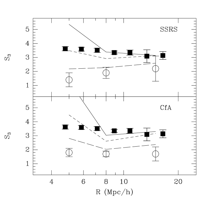
Figure 9: Opened circles show the uncorrected values of $S_{3}$ in the SSRS (top) and CfA (bottom) subsamples at the end of Table 1. These should be compared to the deprojected APM values (filled squares). The lines show the values corrected for the estimation-bias assuming different power-spectrum to estimate the variances $\overline{\xi}_{L}$ and $\overline{\xi}_{2}(R)$ in eq. (29). The LCDM model prediction is shown as a short-dashed line, the linear SCM model as a long-dashed line and the linear APM-like model as a continuous line. All cases are normalized to $\sigma_{8}=1$. The corrections are larger for smaller scales where the measured values are from smaller sub-samples. The SCDM predictions are much lower as it has less power on large scales.

We will concentrate on the last six measurements in Table 1. These published values of $S_{3}$ (Gaztañaga (1992)) are the mean values in the corresponding range of smoothing scales shown in the 4th column. Here we will associate each with the mean value of $R$ in the respective range of scales i.e. $R=5,8$ & $15{\,h^{-1}\,{\rm Mpc}}$ with $S_{3}=1.8,1.7$ & $1.7$ from the CfA50, CfA80 & CfA92 catalogues on the one hand, and $S_{3}=1.4,1.9$ & $2.2$ from the SSRS50, SSRS80 & SSRS115 catalogues on the other. The corrected values of $S_{3}$, adopting the assumptions stated above, are shown as lines in Fig. 9. The correction is larger for the smaller scales which correspond to sub-samples of a smaller size. The SCDM predictions are much lower as it has less power on large scales.

If there is no biasing, we can assume that the APM-values for $\overline{\xi}_{2}$ is close to the true ones, which is is reasonable given the size of the APM (see e.g. Fig. 7). In this case we should concentrate on the continuous line in Fig. 9. At the larger smoothing scales, namely $8$ & $15{\,h^{-1}\,{\rm Mpc}}$, the corrected values are quite consistent with the APM-values. However, at the smallest smoothing scale of $5{\,h^{-1}\,{\rm Mpc}}$, the corrected $S_{3}$’s are significantly higher than the APM-values. Three points should be noted here. First, at this smoothing scale, the correction is so large that the validity of the ansatz expressed in eq. (35) might be called into question. Second, the implicit assumption that the biased- measurements of $S_{3}$ in real- and redshift-space yield similar values should be checked using more simulations. Third, it is in fact well known that the small-scale $S_{3}$ (of the mass) one would infer from an N-body simulation with an APM-like power spectrum and Gaussian initial conditions is larger than the measured $S_{3}$ from the APM survey Baugh & Gaztañaga (1996). One possible interpretation is a scale-dependent galaxy-bias, which tends to diminish on large scales but becomes significant on small scales.

On large scales $R\,\mbox{${}^{>}_{\sim}$}8\,{\,h^{-1}\,{\rm Mpc}}$, we can safely say that most of the discrepancies in existing measurements of $S_{3}$ from the CfA/SSRS/APM catalogues can be explained by an estimation-bias. Remaining differences are attributable to a) a small relative galaxy-bias between the different surveys on large scales; b) redshift-distortions; c) deprojection effects (see Gaztañaga & Bernardeau (1998)) and d) sampling fluctuations. In fact, our analysis as shown in Fig. 8 does support the existence of a galaxy-bias between the CfA/SSRS and the APM. To be strictly consistent, we should have taken this into account in our “correction” of the CfA/SSRS values for $S_{3}$. Doing so is beyond the scope of the present paper. Nonetheless, it should be emphasized that the amount of galaxy-bias one would infer based on measurements of $S_{3}$ is reduced if the estimation-bias is taken into account. A careful assessment would require the inclusion of all the above effects, and ideally, a re-measurement of $S_{3}$ from the different catalogues using methods that are perhaps less prone to the ratio-bias. We hope to pursue these in a future paper.

6 Discussion

The main results of this paper are summarized in eq. (3.1), (3.2) & (3.3), with the associated useful approximations given in eq. (27), (28) & (29). Together they tell us the estimation-biases associated with the standard estimators for the variance $\overline{\xi}_{2}$, the third cumulant $\overline{\xi}_{3}$, and the skewness $S_{3}$ (eq. [11] & [13]). The calculation is based on an expansion in the small parameter $\overline{\xi}_{2}^{L}$ (eq. [17]), which is the variance smoothed on the scale of the survey, but otherwise does not assume or require the smallness of the variance on the scale of interest $R$.

¿From eq. (27), (28) & (29), it can be seen that the standard estimators are all asymptotically unbiased, in the sense that for a given smoothing scale $R$, the estimation-biases tend to zero as the survey-size increases. On the other hand, for a fixed survey-size, the estimation-biases become large as $R$ approaches the size of the survey.

There are two types of terms in the fractional estimation-biases, one dependent on the smoothing scale $R$, being proportional to $\overline{\xi}_{2}^{L}/\overline{\xi}_{2}$ where $\overline{\xi}_{2}$ is the variance smoothed on scale $R$, and the other not, being proportional to $\overline{\xi}_{2}^{L}$ only. In other words, a general form for the estimation bias of an estimator $\hat{E}$ can be represented by eq. (32) where $\alpha_{1}$ and $\alpha_{2}$ are coefficients that depend on the various hierarchical amplitudes, such as $S_{3}$ and $c_{mm^{\prime}}$. For reasonable choices of the parameters $S_{3}$ and $c_{mm^{\prime}}$, the estimation-biases are negative (see Fig. 1). The magnitude of the estimation-biases can be surprisingly large, especially for $E=S_{3}$, because of the large coefficients multiplying $\overline{\xi}_{2}^{L}$ or $\overline{\xi}_{2}^{L}/\overline{\xi}_{2}$.

Our analytical predictions are borne out by numerical experiments discussed in §4. Examples can be found in Fig. 2, 3 & 4. In cases where the estimation-biases are so large that the higher order terms in our expansion in $\overline{\xi}_{2}^{L}$ become important, we show that a simple ansatz works reasonably well (eq. [35]).

In the case of $S_{3}$, we distinguish between two types of contributions to its estimation-bias. The standard estimator for $S_{3}$ is $\hat{S}_{3}=\hat{\overline{\xi}_{3}}/\hat{\overline{\xi}_{2}}^{2}$. Part of the bias arises from the biases of the estimators $\hat{\overline{\xi}_{3}}$ and $\hat{\overline{\xi}_{2}}$ themselves – this is the integral-constraint-bias (eq. [30]). The second part arises from the particular nonlinear combination of these two estimators, which we dub to be the ratio-bias (eq. [31]), or more precisely, the nonlinear-estimation-bias. It turns out the second always dominates on large scales.

We present a preliminary attempt to correct some existing measurements of the variance and skewness in §5. Our main conclusions are a) the apparent increase of the measured variance with survey depth observed by some authors can be nicely explained by the integral-constraint bias (Fig. 8; see e.g. Davis et al. (1988); Gaztañaga (1992); Bouchet et al. (1993)); b) our analysis indicates a small relative galaxy-bias between the CfA/SSRS and the APM galaxies, c) the APM survey should give small estimation-biases for the standard estimator for $S_{3}$ on scales of interest (see Table 1); d) on large scales $R\,\mbox{${}^{>}_{\sim}$}8\,{\,h^{-1}\,{\rm Mpc}}$, most of the differences between the measured skewness from the CfA/SSRS and the APM surveys can be attributed to the estimation-bias; however, a more careful analysis, taking into account redshift-space distortions, relative galaxy-bias (such as due to luminosity segregation) and deprojection effects, is necessary to access the significance of the remaining differences, and whether they are due to pure sampling fluctuations.

Two areas clearly warrant further investigations. First, for the purpose of future surveys such as the SDSS or the AAT 2dF, the $\overline{\xi}_{2}$-independent terms in the estimation biases (the terms associated with $\alpha_{2}$ in eq. [32]) will probably be unimportant, but the $\overline{\xi}_{2}$-dependent terms (the $\alpha_{1}$-terms) can always become important for a sufficiently large smoothing scale $R$. It would therefore be good to have an idea of what that scale is, not just for the variance and the skewness, but also for $S_{N}$ where $N>3$. We will present results for a general N in a separate paper.

Second, we have focused in this paper exclusively on the standard estimators for $\overline{\xi}_{N}$ and $S_{N}$, where $\overline{\xi}_{N}$ is estimated by the standard counts-in-cells technique and $S_{N}$ is estimated by taking the appropriate ratio of ${\hat{\overline{\xi}}}_{N}$ and ${\hat{\overline{\xi}}}_{2}$. There are probably other estimators that suffer from smaller estimation-biases. For instance, Kim & Strauss Kim & Strauss (1998) recently introduced an interesting method to obtain $S_{3}$ by fitting the one-point probability distribution of counts (PDF) using an Edgeworth series. They obtained values higher than previous measurements from the same surveys (see Table 1) indicating that their method is less susceptible to an estimation-bias. An extension of their method using a PDF which is better behaved in the presence of more significant nonlinearities is worth pursuing.

Another possibility which might reduce the ratio-bias in $\hat{S}_{N}$ due to the division of ${\hat{\overline{\xi}}}_{N}$ by ${\hat{\overline{\xi}}}_{2}^{N-1}$: instead of dividing to obtain an estimate of $S_{N}$, fit a curve parametrized in some form to the two-dimensional plot of ${\hat{\overline{\xi}}}_{N}(R)$ and ${\hat{\overline{\xi}}}_{2}(R)$ at each smoothing scale $R$. This is akin to, for instance, how the Hubble constant is usually measured: instead of dividing some estimate of velocity by some estimate of distance for each data point followed by averaging, a linear $\chi^{2}$ fit to all points is performed. This method might give a smaller ratio-bias, but it has to be tested. This procedure has in fact been carried out before by e.g. Gaztañaga Gaztañaga (1992) and Bouchet et al. Bouchet et al. (1993), who obtained values of $S_{3}$ close to that using the standard estimator. But a different parametrization of the relation between ${\hat{\overline{\xi}}}_{N}(R)$ and ${\hat{\overline{\xi}}}_{2}(R)$ (in other words, taking into account carefully the change of $S_{N}$ with $R$) might yield different results.

Perhaps the most important and obvious lesson of our investigation here is that nonlinear combinations of estimators should be used with caution. The only sure-fire way of avoiding an estimation-bias is through Monte-Carlo simulations, such as those performed in §4. There is nothing novel about this point, except that its importance has not been sufficiently emphasized in measurements of certain large scale structure statistics, such as $\overline{\xi}_{N}$ and $S_{N}$ discussed here.

There are also strong interests in measuring such quantities outside galaxy surveys, e.g. for the transmission distribution of quasar spectra and for the convergence distribution in weak-lensing maps. The skewness of the former, for instance, provides a test of the gravitational-instability picture of the Lyman-$\alpha$ forest (Hui (1998)), while the skewness of the latter is a sensitive probe of cosmology (Bernardeau et al. (1997)). Measurements in these areas require similar caution as in the case of galaxy surveys. Our methodology in deriving the estimation-bias for the standard estimator of skewness (ratio of the third cumulant to the second cumulant squared) could be adapted for such measurements (in the case of weak lensing, we learned as this work was being completed that a related calculation was done by Bernardeau et al. (1997)). An important ingredient of our calculation is the use of the hierarchical relation $\xi_{N}\sim\xi_{2}^{N-1}$ in keeping track of the ordering, which might have to be modified for these other applications.

Also, for these applications, as well as for less conventional galaxy surveys such as the Lyman-break galaxy surveys at high redshifts (Steidel et al. (1998)), one often has available several independent fields for which a simple and obvious method should help to reduce much of the ratio-bias of the skewness: measure the third moment and the second moment for each field, separately average each of them over all fields, and only then does one combine these averaged moments to estimate the skewness.

A related suspect of a similar estimation-bias is the measurement of $Q_{N}$, defined as the ratio of the N-point correlation to the sum of suitable permutations of products of the two-point functions (Fry (1984)). The configuration dependence of $Q_{3}$, for instance, provides an elegant test of the galaxy-bias (Fry (1994)). Common ways of estimating it, where estimators are divided by each other, are susceptible to the ratio-bias just as in the case of $S_{N}$. Another possibly problematic statistic is the ratio of the quadrupole to monopole power in redshift-space, or the ratio of the monopole power in redshift-space to that in real-space, which is often used to estimate the parameter $\beta=\Omega^{0.6}/b$ (see review by Hamilton (1997)). An examination of published estimates of $\beta$ show a large scatter even from the same surveys, with maximum likelihood methods yielding consistently higher values (Hamilton (1997)), suggesting an estimation-bias of some sort might be lurking here. It is likely, however, that such attempts to measure $\beta$ are at least equally, if not more strongly, affected by our poor understanding of translinear distortions. We hope to pursue some of the above issues in future work.

We are grateful to Joshua Frieman for useful discussions. This work was in part supported by the DOE and the NASA grant NAG 5-7092 at Fermilab, and by a NATO Collaborative Research Grants Programme CRG970144 between Fermilab and IEEC. EG acknowledges support by IEEC/CSIC, and by DGES (MEC), project PB96-0925.

$R_{0}$	$S_{3}$	$S_{4}$	Scales	Sample	$R_{L}$	Reference
Mpc/h	$(3Q_{3})$	$(16Q_{4})$	Mpc/h		Mpc/h
7	$3.9\pm 0.6$	—	0.5-8	LICK	210	Groth & Peebles 1977
7	—	$48\pm 7$	0.5-4	LICK	210	Fry & Peebles 1978
7	$4.3\pm 0.2$	$31\pm 5$	0.5-4	LICK	210	Szapudi et al. 1992
8	$4-7$	$30-150$	0.1-7	EDSGC	240	Szapudi et al. 1996
8	$4.1\pm 0.1$	$37\pm 2$	0.3-2	APM (17-20)	380	Gaztañaga 1994
8	$3.2\pm 0.2$	$33\pm 4$	7-30	APM (17-20)	380	“
8	$3.1\pm 0.5$	$25\pm 7$	0.5-50	APM (mean)	150-380	Szapudi et.al 1995
10	$2.2\pm 0.2$	$10\pm 3$	4-20	IRAS 1.2Jy	90	Meiksin et al. 1992
6	$2.4\pm 1.1$	$11\pm 13$	2-20	IRAS 1.9Jy	35-60	Fry & Gaztañaga 1994
7	$2.1\pm 0.6$	$7.7\pm 5.2$	3-10	IRAS 1.9Jyz	35-40	“
4-10	$1.5\pm 0.5$	$4.4\pm 3.7$	0.1-50	IRAS 1.2Jyz	30-180	Bouchet et al. 1993
5-10	$2.8\pm 0.1$	$6.9\pm 0.7$	8-32	IRAS 1.2Jyz	30-130	Kim & Strauss 1998
7	$2.4\pm 0.3$	$13\pm 2$	2-10	Perseus-Piscesz	30	Ghigna et.al 1996
—	$2.4\pm 0.2$	—	—	CfA		Peebles 1980 (eq.[57.9])
6	$2.0\pm 0.3$	$6.3\pm 1.6$	1-14	CfA	25- 50	Fry & Gaztañaga 1994
7	$1.9\pm 0.2$	$5.1\pm 1.3$	2-16	CfAz	25-50	“
7	$1.8\pm 0.2$	$5.4\pm 2.2$	1-12	SSRS	25-50	“
8	$1.8\pm 0.2$	$5.2\pm 1.3$	2-11	SSRSz	25-50	“
$5.6\pm 0.4$	$1.8\pm 0.3$	$3.3\pm 1.5$	2-8	CfA50z	25	Gaztañaga 1992
$11.3\pm 0.8$	$1.7\pm 0.2$	$2.5\pm 1.1$	4-12	CfA80z	40	“
$9.8\pm 2.2$	$1.7\pm 0.5$	$3.0\pm 4.3$	8-22	CfA92z	50	“
$6.7\pm 0.5$	$1.4\pm 0.5$	$1.7\pm 2.3$	2-8	SSRS50z	25	“
$9.8\pm 2.0$	$1.9\pm 0.4$	$4.4\pm 2.0$	4-12	SSRS80z	40	“
$11.2\pm 2.5$	$2.2\pm 0.9$	$6.6\pm 8.5$	8-22	SSRS115z	60	“

Table 1: Some measurements of the variance and $S_{N}$, for $N=3,4$, in the literature. The first column $R_{0}$ is the scale at which the measured variance equals $1$. The second and third columns give $S_{3}$ and $S_{4}$, from either counts-in-cells or the multi-point ratios $Q_{N}$, at the scales specified in the fourth column. In most cases, only the mean values for $S_{N}$ over a range of scales were published. In cases where measurements of the individual $S_{N}$ for each smoothing scale are reported in the literature, we quote the actual range of estimates over the corresponding range of scales. An estimate of the effective radius of each sample is given by $R_{L}\equiv(\Omega/4\pi)^{1/3}\cal{D}$, where $\Omega$ is the solid angle of the survey and $\cal{D}$ is taken to be either the maximum depth in volume limited samples or twice the mean depth in magnitude limited samples. The effective volume for IRAS has been divided by two because there are two disconnected polar caps, and measurements were done by averaging the results from the two pieces. Samples with the $z$-superscript are in redshift-space, and those without are in angular-space.

Figure 1: Coefficients $\alpha_{1}$ (continuous line) and $\alpha_{2}$ (dashed line) for the fractional estimation-bias of estimator $\hat{E}$: ${\Delta_{E}\over E}=\alpha_{1}{\overline{\xi}_{2}^{L}\over\overline{\xi}_{2}}+\alpha_{2}\overline{\xi}_{2}^{L}$ (eq. [32]), where $\overline{\xi}_{2}$ is the variance smoothed on scale $R$ and $\overline{\xi}_{2}^{L}$ is the variance smoothed on the scale of the survey. The top panel shows the coefficients for the variance $\hat{E}=\hat{\overline{\xi}_{2}}$ (eq.[27]), and the bottom panel shows the coefficients for the skewness $\hat{E}=\hat{S}_{3}$ (eq.[29]), while the middle panel shows the integral-constraint-bias contribution to $\hat{E}=\hat{S}_{3}$ (eq. [30]).

Figure 2: The integral-constraint-bias of the variance-estimator ${\hat{\overline{\xi}}}_{2}$ in the LCDM model as a function of the smoothing scale $R$. Open circle: the average measured variance, $\langle\hat{\overline{\xi}}_{2}\rangle$, computed from 10 realizations of the full box ($L=300{\,h^{-1}\,{\rm Mpc}}$). Filled triangle: the average measured variance computed using 10 subsamples, each extracted from each realization of the full box ($L=300{\,h^{-1}\,{\rm Mpc}}/M$, for $M=3,4,5$ & $7$ as labeled for each panel). The $1-\sigma$ error-bars are computed from the dispersion of the measured variance around the mean over the 10 respective realizations. Short-dashed line: analytical prediction for the integral-constraint-bias (eq. [27]). Solid line: tree-level PT prediction for $\overline{\xi}_{2}$.

Figure 3: The estimation-bias for $\hat{S}_{3}$ in the SCDM model as a function of the smoothing scale $R$. Open circle: the mean of $\hat{S}_{3}$ over 10 realizations of the full box ($L=300{\,h^{-1}\,{\rm Mpc}}$). Filled triangle: the mean of $\hat{S}_{3}$ over the corresponding subsamples of each realization of the full box (subsample box-sizes are $L=300{\,h^{-1}\,{\rm Mpc}}/M$, for $M=2,4,5$ & $7$ as labeled for each panel). Filled square: the mean of $\hat{\xi}_{3}$ divided by the mean of $\hat{\xi}_{2}^{2}$ over the corresponding 10 subsamples (i.e. the integral-constraint-bias only). The error-bars are computed from the standard deviation of the measured values over the respective 10 realizations; for clarity, error-bars for the squares are only shown in one panel. Short-dashed line: the analytical prediction for the integral-constraint-bias of $\hat{S}_{3}$ (eq. [30]). Long-dashed line: the analytical prediction for the net estimation-bias of $\hat{S}_{3}$ (eq. [29]). Solid line: the tree-level PT prediction for $S_{3}$. Dot-dashed line: a phenomenological ansatz for the net estimation-bias when it becomes large (eq. [35]).

Figure 4: The estimation-bias for $\hat{S}_{3}$ in the LCDM model, labeled in exactly the same way as in Fig. 3.

Figure 5: Measurements of $\overline{\xi}_{2}$ from simulated CfA/SSRS catalogues based on earlier LCDM simulations with $\Gamma=0.2$ (see Fig. 2). Short- and long-dashed lines shows the LCDM simulation results in real and redshift space respectively for the full box ($L=300{\,h^{-1}\,{\rm Mpc}}$). The two sets of point-symbols (one on the left, one on the right) depict the measurements from two different volume-limited simulated catalogues: a) CfA/SSRS50 (for $R\leq 9{\,h^{-1}\,{\rm Mpc}}$), limited to ${\cal{D}}\sim 50{\,h^{-1}\,{\rm Mpc}}$ b) CfA/SSRS90 (for $R\geq 9{\,h^{-1}\,{\rm Mpc}}$), limited to ${\cal{D}}\sim 90{\,h^{-1}\,{\rm Mpc}}$. Square: real space, full sampling ($\sim 10^{4}$ galaxies for CfA/SSRS50 & $\sim 10^{5}$ galaxies for CfA/SSRS90). Open triangle: redshift space, full sampling. Closed triangle with error-bars: redshift space, sparse sampling (200 galaxies). The solid line shows our analytical predictions of the integral-constraint-biases in real-space (eq. [27]) for the respective catalogues. Note that 1. the larger simulated catalogue yields a larger measured variance at $9{\,h^{-1}\,{\rm Mpc}}$; 2. the sparse-sampling does not significantly affect the mean determination of the variance; 3. the real-space and redshift-space biased-estimations of the variance give very similar values.

Figure 6: Measurements of $S_{3}$ from simulated CfA/SSRS catalogues based on earlier CDM simulations with $\Gamma=0.5$ (top panel) and $\Gamma=0.2$ (bottom panel) (see Fig. 2). Dotted line shows the tree-level PT prediction for each model (e.g. $S_{3}=34/7+\gamma$). Short- and long-dashed lines show the measured $S_{3}$ from simulations of the full-box ($L=300{\,h^{-1}\,{\rm Mpc}}$) in real and redshift space respectively. The point-symbols show measurements from two sets of volume-limited simulated catalogues: a) CfA/SSRS50 (left), limited to ${\cal{D}}\sim 50{\,h^{-1}\,{\rm Mpc}}$ b) CfA/SSRS90 (right), limited to ${\cal{D}}\sim 90{\,h^{-1}\,{\rm Mpc}}$. Square: real space, full sampling ($\sim 10^{4}$ galaxies for CfA/SSRS50 & $\sim 10^{5}$ galaxies for CfA/SSRS90). Open triangle: redshift space, full sampling. Closed triangle: redshift space, 200 galaxies. The solid line shows our prediction of the estimation-bias for $\hat{S}_{3}$, using the ansatz introduced in §4.2, in real space. Note how the biased-estimations (from the simulated catalogues) of the skewness give very similar values in real- and redshift-space, even though the true $S_{3}$’s (i.e. measured from the full box) are quite different in the two cases, especially at small smoothing scales.

Figure 7: Measurements of the projected $S_{3}$ (denoted by $s_{3}$ here) from simulated APM-like angular catalogues. Closed circle: the mean of $\hat{s}_{3}$ over 20 angular catalogues from $L=600{\,h^{-1}\,{\rm Mpc}}$ simulations. Open circle: the mean of $\hat{s}_{3}$ over 20 angular catalogues from $L=378{\,h^{-1}\,{\rm Mpc}}$ simulations. Solid line: the tree-level perturbation theory values of the projected $s_{3}$. The agreement of the solid line with the closed circles on large scales indicate that measurements of $s_{3}$ from the large box suffer from negligible estimation-biases. Short-dashed line: the analytical prediction for the estimation-bias of $\hat{s}_{3}$, for the smaller simulation. Long-dashed line: the analytical prediction for the estimation-bias of $\hat{s}_{3}$, for the larger simulation.

Figure 8: The correlation length, defined as $\hat{\overline{\xi}_{2}}(R_{0})=1$, as a function of $R_{L}$ the equivalent radius of the volume limited subsample. Open circles (squares) correspond to the values of the CfA (SSRS) subsamples at the bottom of Table 1. Filled squares correspond to the values in the IRAS 1.2 Jy by Bouchet et al.(1993). The continuous (dashed) line shows the prediction for the measured $R_{0}$, which takes into account the integral-constraint-bias, for the LCDM (SCDM) model, whose power-spectrum-amplitude amplitude is adjusted to fit the data points.

References

- Baugh et al. (1995) Baugh, C. M., Gaztañaga, E., & Efstathiou, G., 1995, MNRAS 274, 1049
- Baugh & Gaztañaga (1996) Baugh, C. M. & Gaztañaga, E., 1996, MNRAS 280, L37
- Bernardeau (1994) Bernardeau, F., 1994, A&A 291, 697
- Bernardeau et al. (1997) Bernardeau, F., Van Waerbeke, L., & Mellier, Y. 1997, A&A 322, 1
- Bernstein (1994) Bernstein, G. M., 1994, ApJ 424, 569
- Bond & Efstathiou (1984) Bond, J. R. & Efstathiou, G., 1984, ApJ 285, L45
- Bouchet et al. (1993) Bouchet, F. R., Strauss, M. A., Davis, M., Fisher, K. B., Yahil, A., & Huchra, J. P., 1993, ApJ417, 36
- Colombi et al. (1994) Colombi, S., Bouchet, F. R., & Schaeffer, R., 1994, A&A 281, 301
- Colombi et al. (1998) Colombi, S., Szapudi, I., & Szalay, A. S., 1998, MNRAS 296, 253
- Dalton et al. (1994) Dalton, G. B., Croft, R. A. C., Efstathiou, G., Sutherland, W. J., Maddox, S. J., & Davis, M. 1994, MNRAS, 271, L47
- Dalton & Gaztañaga (1998) Dalton, G. B., & Gaztañaga, E., 1998, in preparation
- Davis et al. (1988) Davis, M., Meiksin, A., Strauss, M. A., da Costa, L. N., & Yahil, A. 1988, ApJ, 333, L9
- Efstathiou et al. (1992) Efstathiou, G., Bond, J. R., & White, S. D. M., 1992, MNRAS 258, 1P
- Efstathiou et al. (1985) Efstathiou, G., Davis, M., White, S. D. M., & Frenk, C. S., 1985, ApJS 57, 241
- Feldman et al. (1994) Feldman, H. A., Kaiser, N., & Peacock, J. A., 1994, ApJ 426, 23
- Frieman & Gaztañaga (1994) Frieman, J. A. & Gaztañaga, E., 1994, ApJ 425, 392
- Fry (1984) Fry, J. N., 1984, ApJ 279, 499
- Fry (1994) Fry, J. N., 1994, Phys. Rev. Lett. 73, 215
- Fry & Gaztañaga (1993) Fry, J. N. & Gaztañaga, E., 1993, ApJ 413, 447
- Fry & Gaztañaga (1994) Fry, J. N. & Gaztañaga, E., 1994, ApJ 425, 1
- Fry & Peebles (1978) Fry, J. N. & Peebles, P. J. E., 1978, ApJ 236, 343
- Gaztañaga (1992) Gaztañaga, E., 1992, ApJ 398, L17
- Gaztañaga (1994) Gaztañaga, E., 1994, MNRAS 268, 913+
- Gaztañaga (1995) Gaztañaga, E., 1995, ApJ 454, 561
- Gaztañaga & Bernardeau (1998) Gaztañaga, E. & Bernardeau, F., 1998, A&A 331, 829
- Gaztañaga & Fosalba (1997) Gaztañaga, E. & Fosalba, P., 1997, preprint, astro-ph 9712263
- Gaztañaga & Maehoenen (1996) Gaztañaga, E. & Maehoenen, P., 1996, ApJ 462, L1
- Ghigna et al. (1996) Ghigna, S., Bonometto, S. A., Guzzo, L., Giovanelli, R., Haynes, M. P., Klypin, A., & Primack, J. R. 1996, ApJ, 463, 395
- Groth & Peebles (1977) Groth, E. J. & Peebles, P. J. E., 1977, ApJ 217, 385
- Hamilton (1997) Hamilton, A. J. H., 1997, preprint, astro-ph 9708102
- Hockney & Eastwood (1981) Hockney, R. W. & Eastwood, J. W., 1981, Computer Simulation Using Particles, Institute of Physics Publishing
- Hui (1998) Hui, L., 1998, Contribution to the Proc. of Evolution of Large Scale Structure, Garching
- Juszkiewicz et al. (1993) Juszkiewicz, R., Bouchet, F. R., & Colombi, S., 1993, ApJ 412, L9
- Kaiser (1987) Kaiser, N., 1987, MNRAS 227, 1
- Kerscher (1998) Kerscher, M., 1998, preprint, submitted to A&A
- Kim & Strauss (1998) Kim, R. S., & Strauss, M. A., 1998, ApJ 493, 39
- Landy & Szalay (1993) Landy, S. D. & Szalay, A. S., 1993, ApJ 412, 64
- Loveday etal (1996) Loveday, J., Efstathiou, G., Maddox, S. J., & Peterson, B. A. 1996, ApJ, 468, 1
- Meiksin et al. (1992) Meiksin, A., Szapudi, I., & Szalay, A., 1992, ApJ 394, 87
- Munshi et al. (1997) Munshi, D., Bernardeau, F., Melott, A. L., & Schaeffer, R., 1997, preprint, astro-ph 9707009
- Peebles (1980) Peebles, P. J. E., 1980, The large-scale structure of the universe, Princeton University Press
- Silk & Juszkiewicz (1991) Silk, J. & Juszkiewicz, R., 1991, Nature 353, 386+
- Steidel et al. (1998) Steidel, C. C., Adelberger, K. L., Dickinson, M., Giavalisco, M., Pettini, M., & Kellogg, M. 1998, ApJ, 492, 428
- Szapudi (1998) Szapudi, I., 1998, ApJ 497, 16+
- Szapudi & Colombi (1996) Szapudi, I. & Colombi, S., 1996, ApJ 470, 131+
- Szapudi et al. (1996) Szapudi, I., Dalton, G. B., Efstathiou, G., & Szalay, A. S., 1995, ApJ 444, 520
- Szapudi et al. (1996) Szapudi, I., Meiksin, A., & Nichol, R. C., 1996, ApJ 473, 15
- Szapudi & Szalay (1993) Szapudi, I. & Szalay, A. S., 1993, ApJ 408, 43
- Szapudi et al. (1992) Szapudi, I., Szalay, A. S., & Boschan, P., 1992, ApJ 390, 350
- Tegmark et al. (1998) Tegmark, M., Hamilton, A. J. S., Strauss, M. A., Vogeley, M. S., & Szalay, A. S., 1998, ApJ 499, 555+
- Wu et al. (1998) Wu, K. K. S., Lahav, O., & Rees, M. J., 1998, submitted to nature, preprint, astro-ph 9804062