Properties of Galaxy Clusters: Mass and Correlation Functions

Abstract

We analyse parallel N-body simulations of three Cold Dark Matter (CDM) universes to study the abundance and clustering of galaxy clusters. The simulation boxes are $500h^{-1}$Mpc on a side and cover a volume comparable to that of the forthcoming Sloan Digital Sky Survey. The use of a treecode algorithm and 47 million particles allows us at the same time to achieve high mass and force resolution. We are thus able to make robust measurements of cluster properties with good number statistics up to a redshift larger than unity. We extract halos using two independent, public domain group finders designed to identify virialised objects – ‘Friends-of-Friends’ (Davis et al. 1985) and ‘HOP’ (Eisenstein & Hut 1998) – and find consistent results. The correlation function of clusters as a function of mass in the simulations is in very good agreement with a simple analytic prescription based upon a Lagrangian biasing scheme developed by Mo & White (1996) and the Press-Schechter (PS) formalism for the mass function. The correlation length of clusters as a function of their number density, the $R_{0}$–$D_{c}$ relation, is in good agreement with the APM Cluster Survey in our open CDM model. The critical density CDM model (SCDM) shows much smaller correlation lengths than are observed. We also find that the correlation length does not grow as rapidly with cluster separation in any of the simulations as suggested by the analysis of very rich Abell clusters. Our SCDM simulation shows a robust deviation in the shape and evolution of the mass function when compared with that predicted by the PS formalism. Critical models with a low $\sigma_{8}$ normalization or small shape parameter $\Gamma$ have an excess of massive clusters compared with the PS prediction. When cluster normalized, the SCDM universe at z $=1$ contains 10 times more clusters with temperatures greater than $7$keV, compared with the Press & Schechter prediction. The agreement between the analytic and N-body mass functions can be improved, for clusters hotter than 3 keV in the critical density SCDM model, if the value of $\delta_{c}$ (the extrapolated linear theory threshold for collapse) is revised to be $\delta_{c}(z)=1.685\left[(0.7/\sigma_{8})(1+z)\right]^{-0.125}$ ($\sigma_{8}$ is the rms density fluctuation in spheres of radius $8h^{-1}$Mpc). Our best estimate for the amplitude of fluctuations inferred from the local cluster abundance for the SCDM model is $\sigma_{8}=0.5\pm 0.04$. However, the discrepancy between the temperature function predicted in a critical density universe and that observed at $z=0.33$ (Henry et al. 1998) is reduced by a modest amount using the modified Press-Schechter scheme. The discrepancy is still large enough to rule out $\Omega_{0}=1$, unless there are significant differences in the relation between mass and temperature for clusters at high and low redshift.

1 Introduction

Clusters of galaxies, by virtue of being both relatively rare objects and the largest gravitationally bound systems in the Universe, provide stringent constraints on theories of structure formation. The two cluster properties that are most commonly discussed in this context are the abundance and the spatial clustering. The model predictions depend sensitively on the cosmology and on the value of $\sigma_{8}$, the rms density fluctuations on the scale of $8$ $h^{-1}$ Mpc. (Here and throughout this paper, $h$ is the present-day Hubble constant in units of 100 km/s/Mpc.) Comparisons between observations and model predictions have been used to place constraints on cosmological parameters (Strauss et al 1995, Eke, Cole & Frenk 1996, Viana & Liddle 1996; Mo, Jing & White 1996, Borgani et al 1997, De Theije, Van Kampen & Slijkhuis 1998, Postman 1998 ).

It has long been known that clusters of galaxies are much more strongly clustered than galaxies (see, for example, Hauser & Peebles 1973 and review by Bahcall 1988). The two-point correlation function for the clusters is roughly a power law: $\xi_{cc}(r)=(r/R_{0})^{-1.8}$. Bahcall & West (1992) argue that the correlation length, $R_{0}$, obeys the scaling relation

$$R_{0}\approx 0.4D_{c},\ \ 20h^{-1}\,{\rm Mpc}<D_{c}<100h^{-1}\,{\rm Mpc},$$ (1)

where $D_{c}\equiv n_{c}^{-1/3}$ is the mean intercluster separation and $n_{c}$, is the mean space density of clusters. The combined set of results based on the analysis of the spatial clustering of an X-ray flux-limited sample of clusters (Lahav et al.  1989; Romer et al.  1994, Abadi, Lambas & Muriel 1998), of clusters containing cD galaxies (West & Van den Bergh 1991), of richness class R $\geq 0$, R $\geq 1$, R $\geq 2$ Abell clusters (Peacock & West 1992; Postman, Huchra & Geller 1992), and of the cluster samples extracted from the APM Galaxy Survey (Dalton et al.  1992) and Edinburgh-Durham Southern Galaxy Catalogue (Nichol et al.  1992) all give results that are roughly consistent with the above scaling relation.

However, on scales greater than $D_{c}\approx 40h^{-1}\,{\rm Mpc}$, the evidence in favour of the scaling relation hinges just on the analyses of the R $\geq 1$ and R $\geq 2$ Abell cluster samples, which give $R_{0}\approx 21h^{-1}\,{\rm Mpc}$ for $D_{c}\approx 55h^{-1}\,{\rm Mpc}$ and $R_{0}\approx 45h^{-1}\,{\rm Mpc}$ for $D_{c}\approx 94h^{-1}\,{\rm Mpc}$, respectively. Several authors (e.g. Sutherland 1988; Dekel et al.  1989; Sutherland & Efstathiou 1991) have suggested that these correlation lengths have been biased upward by the inhomogeneities and projection effects in the Abell catalogue. However, this suggestion has been rejected by, for example, Jing, Plionis & Valdarnini (1992) and Peacock & West (1992). More recently, Croft et al.  (1997) have analyzed the correlation properties of a sample of “rich” APM clusters and find that the cluster correlation length saturates at $R_{0}\approx 15h^{-1}\,{\rm Mpc}$ ($R_{0}\approx 20h^{-1}\,{\rm Mpc}$ if the analysis is done in redshift-space — see Croft et al.  1997) for $D_{c}>40h^{-1}\,{\rm Mpc}$. The controversy regarding the correlation length of rich clusters: i.e. if the $R_{0}$ vs $D_{c}$ flattens at large scales is as of yet still unresolved.

In an effort to resolve this issue, several authors (e.g. Bahcall & Cen 1992; Watanabe et al.  1994; Croft & Efstathiou 1994, 1997; Walter & Klypin 1996, Eke et al.  1996) have turned to large numerical simulations. Bahcall & Cen (1992) investigated the cluster correlation properties in large N-body simulations of the standard CDM model (SCDM) and two low-$\Omega_{0}$ models ( $\Omega_{0}$ is the density parameter), one spatially flat and one open. They claim to find a linear relation between $R_{0}$ and $D_{c}$ over the range $30h^{-1}\,{\rm Mpc}<D_{c}<95h^{-1}\,{\rm Mpc}$ in all the models but that only in the low-density models is the $R_{0}$-$D_{c}$ relation steep enough to be consistent with the suggested scaling relation (1). More recent works (Croft & Efstathiou 1994, Watanabe et al.   1994) have confirmed that the SCDM model is incompatible with the observed degree of clustering on all scales and for all normalizations. However, no general agreement was reached on the clustering strength at large scales for the other models investigated.

In summary, apart from the general agreement that the SCDM model fails to account for the observed cluster correlations, results obtained from the numerical studies, due to lack of consistency, have been singularly unhelpful in resolving the cluster correlation controversy.

If cluster correlations are going to be used to constrain models of structure formation and place limits on the values of the fundamental cosmological parameters, it is important to understand why these numerical studies give such discrepant results. This is a necessary step before a meaningful comparison between theoretical (numerical) predictions and observations is possible. There are several factors that can affect numerical results and cause the discrepancy described above. Among these are differences in the mass and force resolution of the simulations as well as the overall volume of the simulations. Rich clusters tend to be rare objects and, therefore, simulation studies of the properties of such objects must necessarily span large cosmological volumes. Often, computational limitations require that such simulation studies compromise on the resolution (mass and/or force). However, this can have serious effects on the results. Watanabe et al.  (1994), have shown that degrading the mass resolution tends to bias the correlation lengths downward. Consequently, there is a definite need for analysis of a sample of simulated clusters extracted from a simulation with high mass and force resolution, large number of time steps, and covering a sufficiently large cosmological volume.

In addition to differences in resolution and size, there is the issue of how to identify clusters in the simulations. Bahcall & Cen (1992), Watanabe et al.  (1994) and Croft et al.  (1994; 1997) used different algorithms to identify clusters in their simulations. Using a $\Omega=1$ SCDM model Eke et al.  (1996b) explored the possibility that different algorithms could indeed give different results. They identified and ranked the clusters in their simulations in various different ways, and found that each algorithm/selection criteria imprints its own particular set of biases on the cluster sample; for a fixed value of $D_{c}$, the clustering length can vary up to a factor of $\sim$ 1.5.

In this paper, we report on our analysis of cluster correlations in simulations of both critical density ($\Omega=1$) and open ($\Omega_{0}=0.3$ and $\Omega_{0}=0.4$) CDM cosmogonies and use our results to explore the questions raised above. As described in the next section, both the force and mass resolution of our simulations are better than those of previous studies. Moreover, our simulated volumes are comparable with the Sloan Digital Sky Survey (Loveday 1998) and are larger than the 2dF survey (Colless & Boyle 1998).

We investigate the present-day abundances and temporal evolution of the abundances in the three CDM models. Specifically, we are interested in testing the validity of the widely-used analytic Press-Schechter expression for the cluster mass function. The combination of the present-day abundance of clusters and the rate at which the abundance evolves as a function of time place strong constraints on $\Omega_{0}$ and $\sigma_{8}$. (White, Efstathiou & Frenk 1993; Viana & Liddle 1996; Eke, Cole & Frenk 1996). Since real clusters of galaxies are the product of non-linear gravitational and gas dynamical processes, the most direct way of constraining the range of $\Omega_{0}$ and $\sigma_{8}$ is to carry out large-scale numerical simulations of different models that have the necessary dynamical range and include (poorly known) gas–stellar physics, then “observe” the resulting model universe and compare the simulated observations with the real ones. Computationally, this route is prohibitively expensive at present. A more economical approach involves using the analytic Press-Schechter (PS) formalism (Press & Schechter 1974; Bond et al.  1991) to compute the cluster mass function, map the mass function into an abundance distribution as a function of the observable parameter, and then compare the latter to observations in order to determine the appropriate values of $\Omega_{0}$ and $\sigma_{8}$. Setting aside the uncertainties in the correspondence between mass and an observable quantity, the validity of the analytic approach rests entirely on the assumption that the PS formalism yields an accurate description of the cluster mass function. The analytic expression for the cluster mass function has been extensively tested against numerical simulations in the past (see, for example, Carlberg & Couchman 1989; Lacey & Cole 1994; Klypin et al.  1994, Cole, Weinberg, Frenk & Ratra 1997, Cen 1998) and most studies have found a good agreement between the analytical and the numerical results. However, there have also been some interesting claims to the contrary. Gross et al.  (1998), for example, have drawn attention to a discrepancy between the PS predictions and numerical results at small masses, and Bertschinger & Jain (1994) claim that the PS mass function systematically underestimates the number density of high mass halos. Estimates of parameters such as $\Omega_{0}$ and $\sigma_{8}$ are usually derived from fitting the analytic cluster mass function to the observed distribution. If the PS mass function is indeed failing at the high mass end and this failure is not taken in account, it can affect the determinations of $\Omega_{0}$ and $\sigma_{8}$

In this paper our aim is to determine the halo mass function on group and cluster scales in our set of simulations, and use these to assess the reliability of the analytic PS mass function. Each of our volumes contains several hundred ‘Coma–like’ clusters at the present time. This, in conjunction with our high mass and force resolution, allows us to map out the cluster mass function to high precision out to $z\sim 1$, i.e. over a larger redshift range than previously possible.

The lay-out of the paper is as follows: In §2, we discuss our numerical simulations and the procedure for constructing cluster catalogs. We use these catalogs to extract the cluster mass function and to study their spatial correlation properties. In §3, we present the results of our correlation analyses and in §4, we discuss the cluster mass function. In both sections we compare our numerical results to analytical approximations. Adopting a simple mapping between mass and X–ray temperature, we transform our numerical mass function into a temperature function and highlight the main differences between this temperature function and the one based on the standard Press-Schechter mass function. Finally, we summarize our results and briefly discuss their relevance for future cosmological tests in §5.

2 Numerical simulations and cluster selection

We have simulated structure formation within a periodic cube of comoving length $L=500h^{-1}$ Mpc for two “fiducial” cosmological models: A critical density cold dark matter models ($\Omega_{0}=1$, $h=0.5$ with $\sigma_{8}=1.0$ at $z=0$ ( hereafter we refer to the $\sigma_{8}=0.7$ output as SCDM07 and to the $\sigma_{8}=1$ as SCDM10, respectively. Of course each output of the SCDM run can be rescaled to a different z changing the present day $\sigma_{8}$ normalization) and an open ($\Omega_{0}=0.3$, $h=0.75$, $\sigma_{8}=1.0$ at $z=0$ — hereafter referred to as O3CDM) cold dark matter model. The $z=0.58$ output of O3CDM simulation can, with appropriate rescaling, be identified as an $\Omega_{0}=0.4$, $h=0.65$, $\sigma_{8}=0.79$ CDM simulation (hereafter referred to as O4CDM) of comoving length $L=433.3\;h^{-1}$ Mpc. The same set of simulations was used by Szapudi et al.  (1998) to study the higher order correlation properties of galaxies. The initial conditions were set using the Bardeen et al (1986) transfer function for CDM. The simulations were computed using PKDGRAV, a parallel treecode that allows for periodic boundary conditions and individual time steps (Stadel & Quinn, in preparation). These are among best studied cosmological models (Davis et al.  1985, Jenkins et al.  1997), our choices for the normalization ($\sigma_{8}$) of the open models correspond roughly to those inferred from the present-day cluster abundance (see, e.g., Eke et al. 1996 and references therein), while we analyzed the SCDM simulation data on a $\sigma_{8}$ range that goes from $\sigma_{8}$ = 1 (roughly COBE normalized) to $\sigma_{8}$ = 0.35 (corresponding to z $=$ 1.85 for a $\sigma_{8}$ = 1 at z = 0 model, and to z $=$ 0.43 for a cluster normalized SCDM universe with $\sigma_{8}$ = 0.5 at z = 0) . A cubic spline force softening of 50$h^{-1}$ kpc (43$h^{-1}$ kpc for O4CDM) was used so that the overall structure of clusters could be resolved. Accurate forces were maintained by using a cell opening angle of $\theta<0.8$ (or better at high z) and expanding the potentials of cells to hexadecapole order. Timesteps were constrained to $\Delta t<0.3\sqrt{\epsilon/a}$, where $\epsilon$ is the softening length and $a$ is the magnitude of the acceleration of a given particle. See Quinn et al.  (1997) for a discussion and tests of this timestep criterion. In each run 47 million particles were used, arranged on a 360³ grid. Each run took several hundred hours on 256 nodes of a Cray T3E supercomputer, and about a thousand timesteps. The particle mass is $7.4\times 10^{11}\eta\Omega_{0}h^{-1}\,{\rm M}_{\odot}$, where $\eta=1$ for SCDM and O3CDM models and $\eta=0.65$ for O4CDM. Simulations were started at z $=$ 49. The extremely large volumes simulated, coupled with a reasonable mass resolution and the very good force resolution made possible by the use of a treecode, allow us to study in detail the evolution of structures ranging in size from groups of galaxies, made up of several tens of particles each, to very rich clusters that contain a few thousand particles. In our analyses, we only consider halos consisting of 64 particles or more. This is a stricter constraint than used in most previous work, and was imposed to ensure that our results were not influenced by small-number effects. Finally, we verified that in these simulations both the initial and present–day power spectrum were in close agreement with theoretical expectations ( see Peacock & Dodds 1996).

2.1 Cluster Identification and Selection

Theoretical treatments generally define virialized halos at a given epoch as structures with a mean density averaged over a sphere of $\sim 200$ times the critical density at that epoch (see, for example, Lacey & Cole 1994 and references therein). The mass contained in the sphere is taken to be the mass of the halo and the radius of the sphere is usually identified as the virial radius of the halo.

In numerical simulations, halos are identified using a variety of schemes. Of these, we have chosen to use two that are available in the public domain: FOF (Davis et al. 1985), and HOP (Eisenstein & Hut 1998). These schemes are discussed in the next subsection. Other halo finders that are often used in literature to find virialized halos are DENMAX (Gelb & Bertschinger 1994), the “spherical overdensity algorithm ” or SO, that finds spherically averaged halos above a given overdensity (Lacey & Cole 1994) and the scheme recently developed by Gross et al (1998). The algorithms that we opted to use are those in the public domain and hence, in common use. We felt that it was important to ascertain the extent to which these schemes may bias our results.

2.2 Friend of Friends: FOF

The FOF algorithm (Davis et al.  1985) is one of the most widely used. It is based on a nearest neighbor search. The main advantages of this algorithm are its simplicity and the lack of assumptions about the shape of halos. In this scheme, all particle pairs separated by less than $b$ times the mean interparticle separation are linked together. Sets of mutually linked particles form groups that are then identified as dark matter halos. In the present study, we adopted the linking length that Lacey & Cole (1994) arrived at to identify virialized halos with mean densities of $\simeq 200$ times the critical density at the epoch under consideration. The linking length is $0.2\Omega(z)^{-1/3}$ times the mean comoving interparticle separation. Moreover in the low $\Omega$ models, the scaling of the linking length as a function of redshift was further modified as the mean halo density associated with virialization is a function of redshift (see for example, Kitayama & Suto 1996). The resulting halos also have a mass–radius relation that agrees reasonably well with the theoretical relation for virialized halos (see Lacey & Cole 1994; also, Eke, Cole, Frenk & Navarro 1996). The objects identified by the FOF algorithm are the kinds of objects that the PS formalism refers to (apart from the lack of spherical symmetry) and therefore, we should be able to make a meaningful comparison between the distribution of halos in the simulations and the PS distribution. Several authors have reported the tendency of FOF to link together close binary systems of similar mass especially if the two happen to be loosely connected by a bridge of particles. This pathology can, in specific cases (see for example Governato et al. 1997), give rise to biased results. We have verified that our results are largely unaffected by this problem.

We note that in their study, Lacey & Cole (1994) compared the properties of the halo population defined by FOF and with those of a sample generated using the SO algorithm. They found that at least over the mass range that they could probe using their simulations, the two algorithms gave very similar results.

2.3 HOP

HOP is a recently introduced algorithm (Eisenstein & Hut 1998) based on an hybrid approach. The local density field is first obtained by smoothing the density field with an SPH–like kernel using the n nearest neighbours (we used 16). The particles above a given threshold are linked with their highest density neighbors until, after several “hops”, they are connected to the one particle with the highest density within the region above the threshold. All particles linked to the local density maximum are identified as a group. Like FOF, HOP is well suited to identifing virialized structures once the density threshold is specified to be the local density at the virial radius. Eisenstein & Hut (1998) claim good agreement with the FOF method at masses above the smoothing scale. However, HOP can be tuned to separate binary halos—binary systems loosely connected by one–dimensional particle bridges—thereby avoiding the (rare) FOF pathology.

2.4 FOF vs. HOP

Figure 1: Differential mass function (number density per unit mass) of groups and clusters extracted from the $z=0$ O3CDM simulation volume using FOF (continous line) and HOP (dot–dashed line) algorithms. The dotted line shows the analytic Press-Schechter prediction for the mass function.

In Figure 1 we show the mass functions obtained by applying the two halo finders described to the O3CDM run. The results for SCDM runs are qualitatively similar. The FOF and HOP mass functions agree quite well over the entire mass range probed, with most massive HOP clusters showing a systematic offset of about 7% toward larger masses. This offset can be easily adjusted changing b or the density threshold for HOP. However, as discussed in the above paragraph the parameters used are the most physically meaningful and the small offset is a measure of the kind of biases that you get using different halo finders.

We have found this general agreement to hold for different models and at all redshifts. This result, coupled with results of Eke et al.’s (1996) comparison of the FOF and SO algorithms, strongly indicates that regardless of the actual details of the scheme used to identify the halos, if the resulting halos are independent virialized entities then the statistical properties of the halo populations will be very similar. Figure 1 also shows the PS prediction as a comparison. We defer the comparisons of the theoretical curve to the numerical results in §4.

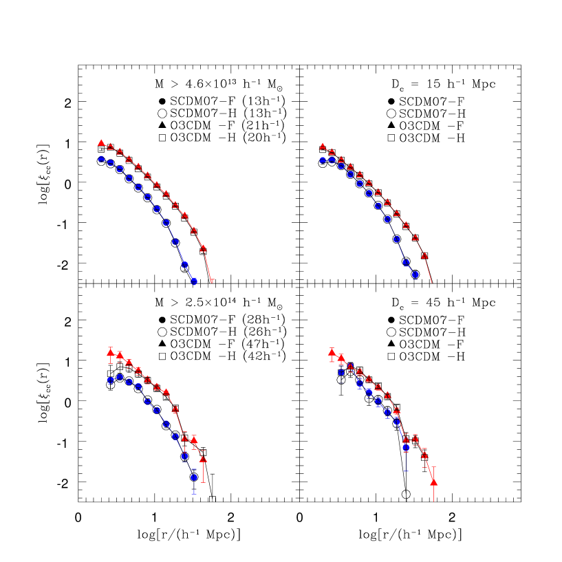
Figure 2: Real-space correlation functions of clusters extracted from the SCDM07 output and O3CDM at z$=$0 using either (F)OF or (H)OP algorithms. The two left panels show the correlation functions for clusters with masses greater than the specified threshold. The numbers in the parenthesis are the $D_{c}\equiv n_{c}^{-1/3}$ values for the cluster samples. The two right panels show correlation functions for samples with the cluster number density given the specified value of $D_{c}$.

3 THE TWO-POINT CLUSTER CORRELATION FUNCTION

The output of our cosmological simulations was processed using the two halo identification algorithms (HOP & FOF) described in the preceding section. We ordered the lists according to halo mass and then generated cluster catalogs by applying a fixed lower mass cutoff. We also generated cluster catalogs based on the ordered list with a specific number density of clusters (labelled by the corresponding value of $D_{c}$).

For each cluster catalog, we compute the real space two-point correlation function using the direct estimator:

$$\xi_{cc}(r)={N_{p}(r)\over n_{c}^{2}V(\delta V)}-1,$$ (2)

where $N_{p}(r)$ is the number of cluster pairs in the radial bin of volume $\delta V$ centered at $r$, $n_{c}$ is the mean space density of the cluster catalog and $V$ is the volume of the simulation. We use all the clusters in our catalogs, taking advantage of the periodic boundary conditions.

The 1$\sigma$ error bars for the correlations are estimated using the formula

$$\delta\xi_{cc}(r)=\frac{3}{2}\frac{1}{\sqrt{N_{cc}(r)}}\left(1+\xi_{cc}(r)\right),$$ (3)

where $N_{cc}$ is the number of distinct cluster pairs in the radial bin at $r$. We have increased the size of the Poisson error bars by $50\%$ because these errors do not take into account clustering and so are likely to underestimate the true errors (Croft & Efstathiou 1994; Croft et al. 1997).

The correlation functions are not well described by a single power-law over the entire range of pair separations sampled. To estimate the correlation length, we fit a functional form

$$\xi_{cc}(r)=\left({r\over R_{0}}\right)^{-\gamma}$$ (4)

over the range $4.5h^{-1}\,{\rm Mpc}<r<25h^{-1}\,{\rm Mpc}$, which brackets the point where $\xi_{cc}=1$. We estimate the value of $R_{0}$ by both fixing the value of $\gamma$ in the above equation to $-1.8$ (see equation 1) and by allowing $\gamma$ to be a free parameter. Since, the fit is done over a restricted range in $r$, both schemes yield similar values of $R_{0}$.

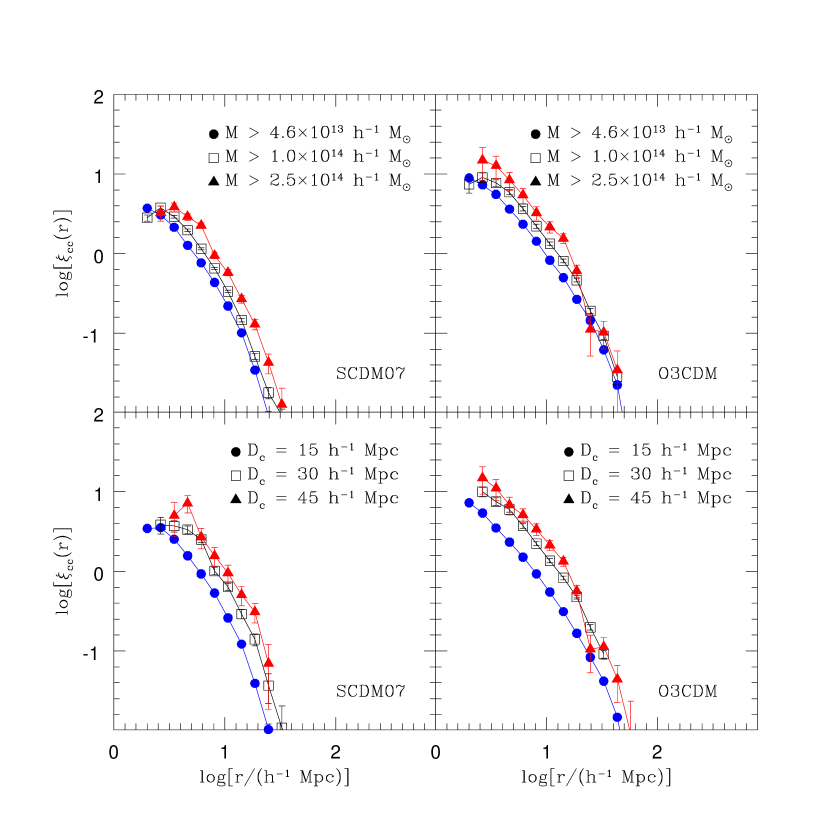
Figure 3: Real-space correlation functions of clusters samples defined by either imposing different mass thresholds (top two panels) or by demanding that the sample clusters have some predefined number density (bottom two panels). The clusters have been extracted from the SCDM07 output and O3CDM at z$=$0 using the FOF algorithm.

In Figure 2, we show real-space correlation functions of clusters in catalogs defined by two different lower mass thresholds ($M_{cut}=4.6\times 10^{13}h^{-1}\;M_{\odot}$ and $2.5\times 10^{14}h^{-1}\;M_{\odot}$) and two different cluster abundance requirements ($D_{c}=15h^{-1}$ Mpc and $40h^{-1}$ Mpc). The clusters are extracted from the simulations using either the FOF or HOP algorithms. Figure 2 shows the results for clusters extracted from the SCDM07 output and the O3CDM simulation at z$=$0; the clustering trends of O4CDM and SCDM10 clusters are the same.

At both low and high mass thresholds, the correlation functions of FOF and HOP clusters are virtually identical, especially in the range $4.5h^{-1}\,{\rm Mpc}<r<25h^{-1}\,{\rm Mpc}$. The abundances of FOF and HOP clusters (or equivalently, their $D_{c}$ value) are also the same, as expected from results shown in Figure 1. As the mass threshold increases, or the number density is decreased, the clustering amplitude increases, but the shape of the correlation function remains the same. This reflects the fact that massive, rare peaks tend to be more strongly clustered in all CDM models. This result is shown in Figure 3.

Given the good match between the halo catalogs we will mainly discuss results for the FOF clusters. Unless specified, results for FOF clusters hold for the HOP clusters as well.

3.1 Cosmology and Normalization of the Mass Power Spectrum

The real-space $z=0$ correlation functions of FOF cluster samples from the various simulations are compared in Figure 4. Considering the SCDM10 and SCDM07 as two z$=$0 outputs results in the model with the higher amplitude (SCDM10) developing structure on group and cluster scales at an earlier epoch, having a higher density of very massive halos and a more strongly clustered mass density field at the present epoch.

In spite of the above mentioned differences, the cluster correlations for the SCDM models with different normalisations are virtually identical in shape and amplitude for cluster samples with both high as well as low mass thresholds. In the case of massive clusters, this has been previously noted by both Croft & Efstathiou (1994) and Eke et al.  (1996). Since for the SCDM models, studying the changes (or lack thereof) in the correlation functions due to variations in the normalization of the amplitude of the primordial density fluctuations is equivalent to studying the evolution of the clustering property as a function of time, we defer the discussion of the above-mentioned until §3.3.

The correlations for the two open models are also very similar to each other, both in shape and amplitude. These two models differ not only in their values of $\Omega_{0}$ and $h$ but also in the normalization of the amplitudes of the primordial mass fluctuations as defined by $\sigma_{8}$. The two OCDM models do, however, have the same value of $\Omega_{0}h^{2}$. Since it is this parameter that defines the position of the peak in the CDM power spectrum characterizing the initial Gaussian random fluctuations in density field, it is perhaps not surprising that the cluster correlations are similar.

In comparison to the cluster correlations in a critical universe, the OCDM cluster correlation functions have a significantly higher amplitude. This occurs because the peak in the power spectrum for the OCDM models is displaced towards larger scales and therefore, for a similar value of $\sigma_{8}$, the OCDM models have more power on large scales than the SCDM models.

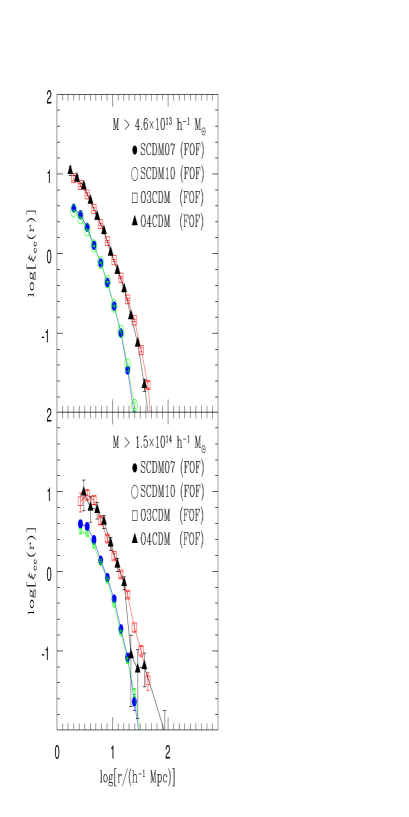
Figure 4: Real-space $z=0$ cluster correlation functions extracted from our simulations (SCDM07, SCDM10, O3CDM, O4CDM) using the FOF algorithm.

3.2 Redshift Evolution

In Figure 5, we plot the present-day and $z=0.43$, $z=0.58$ cluster correlations, in comoving coordinates, for two cluster samples defined as ($M>4.6\times 10^{13}h^{-1}\;M_{\odot}$ and $M>1.5\times 10^{14}h^{-1}\;M_{\odot}$) drawn from the SCDM10 and O3CDM models respectively.

Before we discuss the results, let us consider what is expected. Given a sample of halos with masses greater than some threshold $M_{cut}$, the correlation function of the halos can be related to that of the total mass distribution via the bias parameter: $\xi_{CC}(r;M>M_{cut})=b^{2}_{eff}(M_{cut})\xi_{\rho\rho}(r)$. At a given epoch the bias parameter becomes larger as $M_{cut}$ is raised, as we have already shown. For a fixed $M_{cut}$ and a critical universe, the bias parameter is expected to decrease asymptotically to unity as a function of time (Tegmark & Peebles 1998) as the underlying mass distribution becomes more clustered. The time evolution of $\xi_{CC}(r;M>M_{cut})$ depends on the competition between these two trends.

Figure 5: Correlation functions of SCDM10 and O3CDM clusters computed at two different epochs and plotted in comoving coordinates.

Turning to Figure 5, we note that for both low and high mass thresholds, there are no significant differences between the comoving correlation functions at $z=0$ ($\sigma_{8}$=1) and $z=0.43$ for the SCDM clusters. This implies that over the mass and redshift ranges considered here, the rate of increase in the clustering of the mass distribution is closely matched by the rate at which the bias parameter decreases.

For the O3CDM model, the correlation function at the earlier epoch has a slightly higher amplitude for both low and high threshold samples. The comoving correlation length at $z=0.58$ is a factor of 1.1–1.2 greater.

To summarize, the comoving group/cluster correlation functions are either constant or change very little over the redshift range $0<z<0.5$ and in proper coordinates, the group/cluster correlation length decreases with increasing redshift over the redshift range studied. In the SCDM case, this decrease is given by $R_{0}\propto(1+z)^{-1}$ and in the O3CDM model, by $R_{0}\propto(1+z)^{-0.86}$.

3.3 Comparison with analytic calculations

Table 1: The bias parameter for SCDM07 cluster samples. $b_{1}$ is computed using the standard PS mass function. The second column gives the mass cut in units of the characteristic mass, $M_{*}=4\times 10^{13}h^{-1}\;M_{\odot}$. The final column gives the Lagrangian radius of the halo, which is the smallest separation where the assumtpions in the calculations are valid.

$M_{cut}h^{-1}\;M_{\odot}$	$M_{cut}/M_{*}$	$b_{1}$	$r_{L}h^{-1}$ Mpc
5.7e+14	16.2	3.3	7.9
2.8e+14	7.0	2.4	6.2
2.1e+14	5.2	2.2	5.7
7.0e+13	1.7	1.5	3.9

Table 2: The bias parameter for O3CDM cluster samples. as in Table LABEL:table:bias1. In this case $M_{*}=1.4\times 10^{13}h^{-1}\;M_{\odot}$

$M_{cut}h^{-1}\;M_{\odot}$	$M_{cut}/M_{*}$	$b_{1}$	$r_{L}h^{-1}$ Mpc
2.7e+14	19.3	2.7	9.2
1.9e+14	13.6	2.4	8.2
1.1e+14	7.8	2.0	6.8
9.0e+13	6.4	1.9	6.4
1.8e+13	1.3	1.2	3.7

To date, most studies of cluster correlations have utilized numerical simulations. Such numerical simulations are very expensive to generate, a constraint that renders a systematic exploration of different cosmological models impractical; it also makes it rather difficult to explore and identify the general physical mechanisms underlying the clustering properties of clusters and group halos viz a viz that of the mass distribution. Consequently, various authors (e.g. Kaiser 1984; Bardeen et al.  1986; Mann et al.  1993; Mo & White 1996; Mo, Jing & White 1996, Catelan et al. 1998) have developed analytic schemes to compute the cluster correlation function.

The first method to compute cluster correlation functions analytically that we discuss is based on the Press-Schecter formalism and its extensions. This was originally developed by Cole & Kaiser (1989) and Mo & White (1996) to derive a model for the spatial correlation of dark matter halos in hierarchical models. The calculation consists of three steps (see Baugh et al. 1998).

$\bullet$ Compute the nonlinear power spectrum for the cosmology and $\sigma_{8}$ in question using the transformation of the linear power spectrum suggested by Peacock and Dodds (1996).

$\bullet$ Calculate an effective bias parameter, $b_{eff}$ for the dark matter halos above the specified mass cut as outlined by Mo & White (1996).

$\bullet$ Fourier transform the nonlinear power spectrum to get the nonlinear correlation function of the mass, then multiply by the square of the halo bias factor, to get the real-space, nonlinear, cluster correlation function: $\xi_{CC}(r)=b^{2}_{eff}\xi_{\rho\rho}(r)$.

The cluster correlation function thus computed has been tested, against N-body results by Mo & White (1996) and Mo, Jing & White (1996) and is found to hold even in the mildly nonlinear regime where $\xi(r)>1$ as long as $r>r_{L}$ where $r_{L}=\left(3M/4\pi\rho_{0}\right)^{1/3}$ is the Lagrangian radius of the dark matter halos ($r_{L}\sim 10h^{-1}$ Mpc for rich clusters of galaxies) and $\rho_{0}$ is the present mean density. Recently Jing (1998) has shown that the Mo & White formula systematically underpredicts the bias of low mass halos, but it is in good agreement with numerical simulations in the mass range considered here.

The bias parameter for a dark matter halo that contains a single galaxy is given by the formula derived by Mo & White (1996) and was written down for any redshift in Baugh et al.  (1998):

$$b(M,z)=1+\frac{1}{\delta_{c}}\left[\left(\frac{\delta_{c}}{\sigma(M)D(z)}\right)^{2}-1\right]$$ (5)

Here $D(z)$ is the linear growth factor, normalized to $D(z=0)=1$, $\sigma(M)$ is the rms linear density fluctuation at $z=0$ and $\delta_{c}$ is the extrapolated linear overdensity for collapse at redshift $z$. This gives the bias factor for the halo when the clustering is measured at the same epoch that the halo is identified.

For a sample of halos with different masses, the effective bias is given by

$$b_{eff}(z)={\int N(M,z)\;b(M,z)\;dM\over\int N(M,z)\;dM}$$ (6)

where $N(M,z)\;dM$ is the number density of halos with mass $M$ in the sample. For the cluster samples that we have constructed, $N(M,z)$ can either be set equal to the Press-Schechter mass function (with $\delta_{c}$ set to the canonical value defining collapse for the cosmology under consideration) or to the cluster mass function computed directly from the cluster catalogs. However the results shown here are almost insensitive to this choice.

The effective bias parameters for samples whose correlation functions are plotted in Figure 6 are given in Tables LABEL:table:bias1 (SCDM07) and LABEL:table:bias2 (O3CDM). The mass cuts applied correspond to halos of different rarity in the two cosmologies; this is quantified by comparing the mass cut to the characteristic mass $M_{*}$, which is defined later in §4. All the mass cuts considered correspond to objects that are greater than $M_{*}$, and so these halos are biased tracers of the dark matter distribution (Mo & White 1996). The cluster sample with the highest mass cut for both O3CDM and SCDM07 is predicted to have a correlation function that is $\sim 10$ times higher than that of the dark matter.

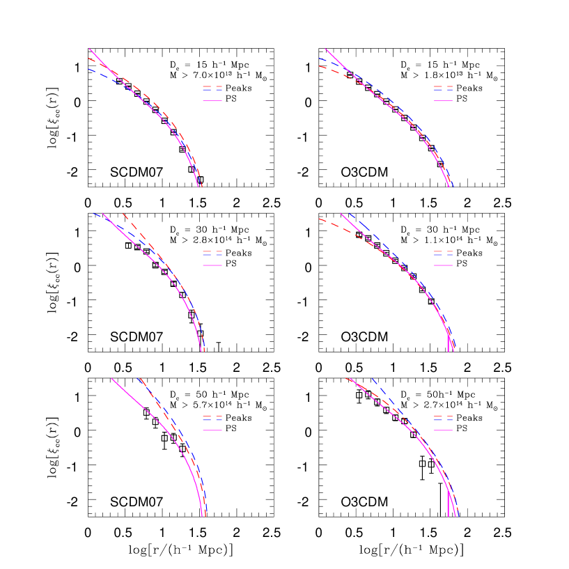
Figure 6: Analytic correlation functions compared against our numerical results. The two dashed curves are the peaks-based correlation functions computed according to the prescription of Mann et al.  (1993). The curve with the higher correlation amplitudes on small scales corresponds to $\delta_{c}=1.7$. The other curve corresponds to $\delta_{c}=1.$. The two solid curves are the PS-based correlation functions computed as described in §3.5. The correlation functions are computed assuming either the standard PS mass function or the numerical cluster mass function (see §4). The two are very similar.

The PS-based analytic correlation functions are shown in Figure 6 as solid curves. There is little difference between the correlation functions computed using the standard PS mass function and the numerical mass function discussed in §4. The analytic correlations are in excellent agreement with our numerical correlation functions. The agreement between the numerical and analytic results is further confirmed by the match between the analytic and numerical $R_{0}$–$D_{c}$ curves. The analytic $R_{0}$–$D_{c}$ curve is plotted in Figures 7 and 8 as the light solid curve.

We consider next the scheme developed by Mann et al.  (1993). This is based on the method devised by Couchman & Bond (1988; 1989) that combines the theory of the statistics of peaks in Gaussian random fields with the dynamical evolution of the cosmological density field.

In this scheme, the time evolution of the density field is followed using the Zel’dovich approximation (Zeldovich 1970). At the epoch of interest, a particular class of objects is defined by the pair $R_{s}$ and $\delta_{c}$. These are, respectively, the smoothing scale that is applied to the cosmological density field and the linearly extrapolated amplitude of the density fluctuations at the time of collapse. Mann et al.  (1993) set the values of these two parameters by choosing an appropriate value for $\delta_{c}$ ($\delta_{c}=1.686$, corresponds to collapse of spherical density perturbations in an $\Omega_{o}=1$ universe) and then adjusting $R_{s}$ until the number density of peaks with overdensities greater than $\delta_{c}$ corresponds to number density of objects under consideration. Full details can be found in Mann et al.  (1993).

In Figure 6, we plot the correlation functions of some of our cluster samples and show the corresponding analytic peaks-based correlation functions computed assuming $\delta_{c}=1$ and $\delta_{c}=1.7$ (dashed curves) according to Mann et al.  (1993)’s prescription.

Figure 7: Cluster correlation length as a function of $D_{c}$, the mean cluster separation, for clusters extracted from the SCDM07 output using FOF (heavy solid curve). The error bars show the 1$\sigma$ errors in $R_{0}$ derived from fitting the correlation functions with a $-1.8$ power-law as described in the text. The solid line corresponds to the scaling relation between $R_{0}$ and $D_{c}$ (equation 1) advocated by Bahcall & West (1992). The dot–dashed line shows the $R_{0}$–$D_{c}$ that Bahcall & Cen (1992) derived from their numerical study. The short-dashed curve corresponds to the numerical results of Croft & Efstathiou (1994). In addition, the open triangles show the results for R$\geq 0$, R$\geq 1$ and R$\geq 2$ Abell clusters (Bahcall & Soneira 1983; Peacock & West 1992) and the open circles show the results for APM clusters (Dalton et al.  1992; Croft et al.  1997). The light solid curve is the $R_{0}$–$D_{c}$ relation derived from analytic PS-based correlation functions computed according to the prescription in Baugh et al.  (1998) — see §3.5.

As noted by Mann et al.  (1993), the correlation functions computed using $\delta_{c}=1.7$ consistently overestimate the correlation amplitudes on all scales of interest. The correlation functions for $\delta_{c}=1$ are in excellent agreement with the numerical results for $D_{c}\leq 30h^{-1}$ Mpc (however, a value of $\delta_{c}\sim 1$ is rather unphysical). For larger values of $D_{c}$, the analytic results tend to overestimate the correlations, with the discrepancy first becoming obvious on small scales and then propagating out to larger scales as $D_{c}$ continues to increase. For a given $D_{c}$, the discrepancy is more severe for SCDM07 clusters than for O3CDM clusters.

The tendency for the peak scheme to overestimate the correlations on scales where $\xi_{CC}(r)\geq 1$ by a margin that grows larger with increasing $D_{c}$ suggests that the peaks-based method will overestimate the correlation lengths of samples with large values of $D_{c}$. Both Mann et al.  (1993) and Watanabe et al.  (1994) have computed the $R_{0}$–$D_{c}$ relation predicted by the peaks method. Comparing their $R_{0}$–$D_{c}$ curves for O3CDM-like models with our numerical results we find that for cluster samples with $D_{c}\approx 80h^{-1}$ Mpc, the correlation length predicted by the peaks-based analytic scheme is $R_{0}\approx 28h^{-1}$ Mpc whereas the simulation result is $R_{0}\approx 22h^{-1}$ Mpc, very close to the PS based prediction. The breakdown in the peak scheme may be due to several factors. The simplest possibility is that that the method uses the number density of clusters in a sample as a constraint rather than some physical properties of the clusters such as their masses. Other possible causes of the breakdown are: the manner in which the different filtering scales are chosen, the simplistic nature of the prescription defining the relation between peaks in the smoothed density field and “clusters”, and the requirement that the large–separation asymptotic limit of the statistical contribution to the cluster correlation function matches the statistical peak–to–peak correlation function (Mann 1998, private communications). The latter two tend to magnify any minor discrepancy caused by any of the other factors.

3.4 Correlation Length and the Cluster Abundance

In Figures 7 and 8, we plot correlation length ($R_{0}$) as a function of cluster abundance in terms of $D_{c}$, the mean cluster separation, for the FOF clusters in the SCDM07 output and O3CDM model at z$=$0. For comparison, we also show the scaling relation (Equation 1); the numerical results of Bahcall & Cen (1992) and Croft & Efstathiou (1994) the observational data for R$\geq 0$, R$\geq 1$, R$\geq 2$ Abell clusters (open triangles) from Bahcall & Soneira (1983) and Peacock & West (1992) and the data for the APM clusters (open circles) given by Dalton et al.  (1992) and Croft et al.  (1997). In neither of the SCM07 nor O3CDM models is the $R_{0}$–$D_{c}$ relation for clusters consistent with the scaling relation $R_{0}=0.4D_{c}$.

Figure 8: Same as Fig. 7 but for O3CDM model.

However, it should be noted that the numerical results show the $R_{0}$–$D_{c}$ relation for the real-space correlation function whereas the correlation lengths for the observed clusters are derived from redshift-space correlation functions. Redshift–space correlation lenghts are generally larger than their real-space correlation length counterparts. For example, in the case of their low-density spatially flat CDM model, Croft & Efstathiou found that their real-space $R_{0}$-$D_{c}$ relation saturates at $R_{0}\approx 15h^{-1}$ Mpc for large values of $D_{c}$, whereas the redshift-space $R_{0}$-$D_{c}$ saturates at $R_{0}\approx 21h^{-1}$ Mpc. An increase of this kind, however, is not sufficient to bring our numerical $R_{0}$–$D_{c}$ relation into agreement with the scaling relation of equation 1.

Consistently with all previous findings, the $R_{0}$-$D_{c}$ curve for clusters extracted from the SCDM universe (Figure 7) does not match either the APM or Abell results. On the other hand, the results of our O3CDM model are in good agreement with the APM and richness R$>0$, R$>1$ Abell cluster data, even if the effect of redshift distorsions increasing the length scale $R_{0}$ a few Mpc were included.

The seriously discrepant datapoint is for R$>2$ Abell clusters. If this measurement is correct, it suggests that clustering on very large scales may have been modulated by non-Gaussian processes (see Mann et al.  1993; Croft & Efstathiou 1994) as it is very difficult to conceive of a Gaussian model that can produce the requisite clustering at these scales. It would also imply that the very rich APM clusters with their comparitively large correlation lengths are not really rich or massive systems but rather are systems comparable to R$>1$ Abell clusters whose number densities have been biased downward by the cluster identification algorithm. The agreement between our analytic results and our numerical results for clusters in the O3CDM model and the APM results leads us to believe that it is the R$>2$ Abell result that is most likely incorrect, biased upward by the inhomogeneities and contamination due to projection effects in the Abell catalog as argued by Sutherland (1988) and Sutherland & Efstathiou (1991).

In comparing our numerical results for SCDM07 to those of Bahcall & Cen (1992), we find that for $25h^{-1}$ Mpc $<D_{c}<40h^{-1}$ Mpc, our $R_{0}$-$D_{c}$ results are consistent with theirs. For $D_{c}>40h^{-1}$ Mpc, our curve rises less steeply than that of Bahcall & Cen and appears to saturate for $D_{c}>50h^{-1}$ Mpc. From analytic results (light solid curve), which we discuss further in the next subsection, we expect the $R_{0}$-$D_{c}$ curve to continue to rise but much more gently than the Bahcall-Cen result. Since both we and Bahcall & Cen (1992) used the FOF algorithm to identify clusters in the simulations, the cluster selection algorithm cannot be responsible for the differences. Furthermore, our correlation lengths were determined in the same way as Bahcall & Cen (1992).

Comparing our O3CDM results to those of Bahcall & Cen’s (1992) low-$\Omega$ models, we find that the two are in good agreement for $D_{c}<35h^{-1}$ Mpc and also in a rough agreement with the scaling relation. However as the cluster abundance decreases and $D_{c}$ increases, the correlation lengths of our cluster samples do not increase as quickly. Our numerical results at large values of $D_{c}$ are in good agreement with those derived analytically to the scales probed by our simulations. (see §3.3)

In comparing our $\sigma_{8}=0.7$ result to Croft & Efstathiou’s (1994) $r_{c}=1.5h^{-1}\,{\rm Mpc}$ $\sigma_{8}=0.59$ SCDM model, we once again find smaller correlation lengths for $D_{c}<30h^{-1}\,{\rm Mpc}$. For higher values of $D_{c}$, the Croft & Efstathiou (1994)’s results are consistent with ours in spite of the fact that we have used FOF to identify the clusters and Croft & Efstathiou (1994) results are based on a very different scheme. Comparing our O3CDM results to those of Croft & Efstathiou’s (1994) $1.5h^{-1}\,{\rm Mpc}$, $\sigma_{8}=1.0$ low-$\Omega$ spatially flat CDM model, we find that within the uncertainties in the two curves, they are in excellent agreement with each other. The flattening in Croft & Efstathiou’s curve for $D_{c}>50h^{-1}\,{\rm Mpc}$ (at $R_{0}\approx 15h^{-1}\,{\rm Mpc}$) is not real. As indicated by both our numerical and analytic results, the correlation continues to rise, albeit gently, reaching $R_{0}\approx 22h^{-1}$ Mpc at $D_{c}=80h^{-1}$ Mpc and is still rising. The flattening trend is likely an artifact of the finite simulation volume or even the poor mass/force resolution.

4 THE CLUSTER MASS FUNCTION

According to the analytic PS formalism, the comoving number density of dark matter halos of mass $M$ in the interval $dM$ is

$${N(M)}=\sqrt{2\over\pi}{\bar{\rho}\over M^{2}}{\delta_{c}D^{-1}\over\sigma}\left|{d\ln\sigma\over d\ln M}\right|\exp\left[-{\delta_{c}^{2}D^{-2}\over 2\sigma^{2}}\right],$$ (7)

where $\bar{\rho}$ is the comoving density of the Universe and $\sigma(M)$ is the linearly extrapolated present-day $rms$ density fluctuation in spheres containing a mean mass $M$. The redshift evolution of $N(M)$ is controlled by the density threshold for collapse, $\delta_{c}/D(z)$, where $D(z)$ is the linear growth factor normalized to unity at $z=0$ (Peebles 1993) and $\delta_{c}$ is the linearly evolved density contrast of fluctuations that are virializing at $z=0$. The growth factor, $D(z)$, depends on $\Omega_{0}$ and $\Lambda$ whereas $\delta_{c}$ has only a weak dependence on $\Omega_{0}$. For spherical density fluctuations, $\delta_{c}=1.686$ for $\Omega_{0}=1$ and $1.65$ for $\Omega_{0}=0.3$.

The PS description of structure formation in the Universe leads naturally to the definition of a characteristic mass $M_{*}(z)$ such that

$$\sigma(M_{*})D(z)=\delta_{c}\,.$$ (8)

$M_{*}(z)$ is then the characteristic mass of halos that are virializing at redshift $z$. Its evolution tracks the manner in which structure forms. In bottom-up hierarchical clustering models, such as CDM models, $M_{*}(z)$ increases as a function of time as lower mass structures are incorporated into progressively more massive halos. In a critical universe, the growth factor evolves as $D(z)=(1+z)^{-1}$ and to first order, this implies a strong evolution in $M_{*}$. In an open or a flat, low-$\Omega_{0}$ universe, $D(z)$ ceases to evolve as strongly, and the evolution of the characteristic mass is greatly suppressed, once $\Omega(z)$ deviates significantly from unity. Hence, the evolution of the dark halo mass distribution is also greatly suppressed. A clear detection of the presence or absence of strong dynamical evolution in the cluster population can be used to put stringent limits on the underlying cosmology.

The actual value and the details of the evolution of $M_{*}$, and therefore of the mass distribution especially for $M>M_{*}$, depends sensitively on $\delta_{c}$. The standard practice is to use the value of $\delta_{c}$ for collapse of spherical perturbations. Typical perturbations in CDM models, however, are not spherical and therefore, the actual value of $\delta_{c}$ will differ from the spherical value. Moreover, Heavens & Peacock (1986), argue that $\delta_{c}$ is likely to be lower ($1\leq\delta_{c}\leq 1.68$) because typical proto-structures in a Gaussian random field tend to be triaxial. A lower (higher) value of $\delta_{c}$ results in more (fewer) high mass objects. A detailed discussion of $\delta_{c}$ and the asphericity of the density perturbations is given by Monaco (1995, 1998), who finds that when the assumption of spherical collapse is relaxed, $\delta_{c}$ becomes a function of the local shape of the perturbation spectrum. In most cosmological models, the power spectrum of the primordial perturbations over the scales of interest deviates, albeit gently, from a simple power law shape and it becomes debatable whether a constant value of $\delta_{c}$ is a fair description of the evolving cosmic mass function at all masses and redshifts. Here we allow the collapse threshold to be a free parameter depending on redshift, calibrating at each epoch using the high mass end of the mass distribution. As discussed in §1 and §2.3, the halo mass function derived using the PS formalism is a measure of the abundance of collapsed, distinct, halos characterized by their virial radius and mass. Consequently, it is appropriate to use catalogs generated using the FOF and HOP cluster finding algorithms.

4.1 Computing the halo mass function

We construct the differential mass function by sorting the halos according to their masses in bins of size $\Delta$log(M) = 0.1. We have verified that our results are insensitive to this choice of bin size. Due to the large size of our simulations, we are able to study also the differential cluster mass function instead of the cumulative distribution, as is usually done. This means that the individual bins are independent and the results more robust. We estimate the uncertainty in the number of objects in each bin using Poisson statistics. It is useful to remember that the SCDM run can be rescaled freely to a different $\sigma_{8}$ normalization, The redshift of each given output is then rescaled to a redshift z’: $1+z^{\prime}=(1+z)/\sigma_{8}$.

4.2 Effects of numerical resolution and cosmic variance

To study the effects of degrading the numerical resolution, we examined a lower resolution run of our SCDM07 volume. This run used the same phases, 3 million particles, a softening length of $160h^{-1}$ kpc and a third of the timesteps used in our fiducial run. Both force and spatial resolution are therefore significantly poorer. Halos represented by 128 particles in our fiducial run have only 8 particles in the low resolution simulation. While there is good agreement at the high mass end, the low mass end of the mass function is severely affected by the poorer resolution, showing a significant decrease in the number density of halos below $3\times 10^{14}h^{-1}M_{\odot}$. This test indicates that at least 30 particles are needed to correctly assign a mass to individual halos. Our choice to include in our analyses only halos with N$>64$ is then a conservative one.

Finally, we also explored the effects of cosmic variance on the cluster number density. We divided our $z=0$ SCDM07 volume into several subvolumes and measured the local $\delta_{c}$ over the same mass range as we did for the whole volume. As expected, cosmic variance produces a scatter in $\delta_{c}$ when measured in smaller volumes. However the scatter is not significant for volumes as little as $1/8$-th of the original simulation volume (i.e. cubes with 250h^-1Mpc per side): we find $\delta_{c}$ = 1.68 $\pm$ 0.02. This is close to the error associated with a single measurement and similar to the value we get from the whole volume, suggesting that the value of $\delta_{c}$ for a given halo finder has (almost) converged when the full volume of the simulation is considered.

4.3 Press-Schechter Predictions vs Numerical Results

Figure 9: The N-body mass distribution for the SCDM run — shown as points — at four different outputs as well as the standard PS mass function (computed using $\delta_{c}=1.686$) — shown as lines — for the same four outputs: $\sigma_{8}=1$ (filled circles, solid line), $\sigma_{8}=0.7$ (circles, dotted line),$\sigma_{8}=0.47$ (squares, dashed line), $\sigma_{8}=0.35$ ( triangles, long dashed line). The error bars correspond to 1$\sigma$ Poisson errors.

Figure 10: The same as Figure 9 but for O3CDM model at z=0,0.58,1.

In Figures 9 and 10, we show the differential mass functions from the SCDM and O3CDM simulations, respectively. The corresponding PS curves, computed using the canonical value of $\delta_{c}$ for spherical perturbations, are also shown. We only show the FOF results. Generally, the HOP and FOF results are very similar, with HOP having a slightly larger number of massive clusters.

In the case of the SCDM model, we find that the shape of the differential PS mass function is roughly consistent with the shape of the numerical mass function only at $\sigma_{8}=1$ At lower $\sigma_{8}$ (or alternatively, higher z) the PS mass function underestimates the number density of rich clusters in the simulation. The excess at the high mass end is about a factor of a few in number density per mass bin. At $\sigma_{8}$ 0.7 or larger the PS approach overestimates the number of small halos (M $<10^{14}h^{-1}\;M_{\odot}$). The deficit of low mass halos (which we will only touch upon briefly here) has been well-documented in numerical works by Carlberg & Couchman (1988) and more recently, by Lacey & Cole (1994), Gross et al.  (1998) and Somerville et al.  (1998). This deficit arises independently of the choice of algorithm used to define the halos in the simulations (see Figure 1) and has been associated with merger events not accounted for by the PS formalism (see Cavaliere & Menci 1997 and Monaco 1997). The fact that the two halo finders agree extremely well in this regime makes the result very robust.

Apart from the above-mentioned deficit, most other studies that have tested the analytic PS mass function against numerical results have reported a good agreement between the two (e.g. Eke et al.  1996) with the notable exceptions of Bertschinger & Jain (1994) and Sommerville et al.  (1998), who found a systematic excess of massive halos in numerical simulations as compared to the PS prediction. These numerical results, however, are derived from simulations that have lower resolution and probe smaller cosmological volumes than our simulations. These simulations, consequently, contain only a small number of massive clusters and this, in conjunction with cosmic variance, has resulted in numerical mass functions with large uncertainties at the high mass end. Eke et al.  (1996), found a good agreement with the PS mass function on the scale of $5\times 10^{14}h^{-1}M_{\odot}$ but with a large error bar.

The large volumes used in our work allow us to confirm the good agreement between the numerical and the analytical mass function found for high values of $\sigma_{8}$. The excess of massive clusters at lower $\sigma_{8}$/higher redshifts suggest that the cluster mass function for the SCDM model evolves more slowly than the PS mass function. At $\sigma_{8}$=0.35, the number density of Coma–like clusters exceeds the standard PS prediction by almost an order of magnitude. Allowing $\delta_{c}$ to be a free parameter at each epoch, we perform a $\chi^{2}$ fit of the PS formula to the numerical results assuming Poisson errors for each bin. Since observations tend to be biased towards the high-mass end, we include in our fit only clusters with temperature T$>$3keV, (the M–T relation is defined in §4.4) to allow the use of this formula in theoretical predictions for X-ray clusters. This formula will underestimate slighlty the number of very (T$>$7keV) hot clusters for high $\sigma_{8}$ models.

For the SCDM cluster mass function at $\sigma_{8}$=0.7 , the best–fit $\delta_{c}$ coincides with the canonical value of $1.686$ ! For $z>0$ and for our FOF selected halos, the best-fit value of $\delta_{c}$ as a function of redshift and $\sigma_{8}$ is :

$$\delta_{c}(z)=1.686\left[\left(\frac{0.7}{\sigma_{8}}\right)(1+z)\right]^{-0.125}$$ (9)

as shown in Figure 11, whereas the canonical value of $\delta_{c}$ is a constant. (in Figure 11 errorbars are 3 $\sigma$ errors). For HOP selected halos $\delta_{c}$ is offset toward even lower values, i.e. toward a larger cluster excess: $\delta_{c}=1.6$ at z$=$0. (for the SCDM model at $\sigma_{8}=0.7$). However, a similar evolution of $\delta_{c}(z)$ is found, with a $(1+z)^{-0.1}$ dependence. In principle the fitting procedure should keep into account that the mass associated with a given temperature depends on z and that the same output can be associated with different z depending on $\sigma_{8}$. However the fitting formula is not affected by this for values of present day $\sigma_{8}$ between 1 and 0.5 and eq. 9 can be used safely.

In the O3CDM model case , the PS mass function is in fair agreement with the numerical mass function, especially at low redshifts. At $z=0$, the high mass end of the numerical halo mass function agrees within 2$\sigma$ with the analytical curve computed using the canonical (spherical) value of $\delta_{c}$ = 1.651. The uncertainties in the number densities of massive clusters are slightly larger in the O3CDM case because of the smaller physical volume/h igher H₀ of the simulation. As shown in Figure 11, the best-fit $\delta_{c}(z)$ for FOF halos can be well-approximated as

$$\delta_{c}(z)=1.775(1+z)^{-0.07}$$ (10)

HOP results shows an even weaker evolution in z. As the result is more significant in the SCDM case we will mainly focus on the analysis of results for the critical case.

Figure 11: The points show best fit values of $\delta_{c(z)}$ required to match the numerical mass function for clusters with T$>3$ keV at different redshifts. The squares show the results for the SCDM07 model and the triangles show the results for O3CDM model. The horizontal light solid curve and the nearly horizontal dashed lines show the canonical values of $\delta_{c}(z)$ for the SCDM07 and the O3CDM models respectively. The lines across the points are the power-law interpolation to the points (see text). Bars are 3 $\sigma$ errors.

Figure 12: The points show the best-fit values $\delta_{c}(z)$ for SCDM07 (continuous) and O3CDM (dashed) at z=0 (black dots) and z=1 (i.e $\sigma_{8}=0.35$ for SCDM) (open squares) as the mass range over which the PS functional form is fitted to the numerical FOF mass function is varied. The abscissa corresponds to the lower mass threshold of the mass range over which the fit is demanded.

From these results however, it is not clear if the deviation from the standard PS mass function is due to just one or rather both of the following effects:

$\bullet$ at lower $\sigma_{8}$ and for a fixed temperature T we study more extreme clusters i.e. we look at a different region of the mass function, which maybe still be self similar, albeit different from the canonical PS.

$\bullet$ the shape of the mass function evolves with time and/or depends on the power spectrum

As discussed above, the best-fit $\delta_{c}(z)$ were determined by fitting the functional form of the PS mass function to the numerical results for clusters with T$>3$ keV, i.e. on mass scales $M\gg M_{*}$, where $M_{*}$ corresponds to $4\times 10^{13}\,h^{-1}M_{\odot}$ for SCDM07 and $1.5\times 10^{13}\,h^{-1}M_{\odot}$ for O3CDM. It is of interest to relax this constraint and explore how the $\delta_{c}$ varies as the minimum mass of the halos included in the fit is lowered and approaches the mass of the smallest halos (64 particles) in our catalog. We carried out the above exercise at two different epochs/normalization and the results are shown in Figure 12. The value of $\delta_{c}$ changes dramatically as the mass range over which the fit is carried out moves toward smaller masses (the fit is dominated by the smaller mass bins as they contain most of the halos used in the fitting). The trend for both SCDM and O3CDM is for $\delta_{c}$ to become larger as the mass threshold is lowered. This is precisely what one expects given the deficit of low-mass halos in the simulations. This shows that the shape of the N–body mass function differs from the PS prediction, and the exact value of $\delta_{c}$ is a function of the mass interval considered.

This plot shows also that, at a given mass, $\delta_{c}$ is a function of redshift. To prove that the shape of the mass function evolves with time we take advantage of the fact that within the PS framework the cumulative fraction of mass in collapsed halos is invariant when plotted vs the variance of the density field at a given mass/lenght scale. I.e. at a given value of $\sigma$ (which corresponds to different mass/lenght scales depending on cosmology and z) the fraction of mass in collapsed objects is always the same. This is shown in Figure 13.

Figure 13: The plot shows the cumulative fraction of mass in collapsed halos as a function of the variance of the density field. The PS prediction (invariant with redshift and cosmology) is the thick continuous line. The SCDM results are shown at diffferent outputs: $\sigma_{8}=1$: dot–long dashed; $\sigma_{8}=0.7$: dot–short dashed; $\sigma_{8}=0.47$: dottted line; $\sigma_{8}=0.35$: dashed. The numerical mass function is obviously not invariant and shows evidence of evolution.

It is interesting to interpret this change in terms of different power spectra. SCDM models can be rescaled to models with different $\Gamma^{\prime}$ (or $\tau$CDM models) rescaling the box by $\Gamma/\Gamma^{\prime}$ and choosing as the final output the one with the correct present–day normalization at the scale corresponding to the 8h^-1Mpc scale. The sequence of outputs with decreasing $\sigma_{8}$ and increasing excess of massive objects can be reinterpreted as a sequence of models with smaller $\Gamma$ parameter and the same normalization, revealing the dependence of the shape of the mass function from the power spectrum. An excess of massive halos for a more negative local spectral index (as the case with larger $\Gamma$) had been predicted by Monaco (1995).

This rescaling allowed to compare our mass functions with that obtained from the so called “Hubble Volume Simulation” (HVS) (Colberg et al.  1998), a $\tau$CDM with $\Gamma$=0.21 and normalization of $\sigma_{8}=0.6$ Their final output can be rescaled to a SCDM model with a $\sigma_{8}=$ 0.285. The HVS mass function lies nicely along our sequence of mass functions (Cole & Jenkins 1998, private communication) showing a slightly larger excess of halos compared to our $\sigma_{8}=0.35$ output (our output with the lowest $\sigma_{8}$).

The two simulations used completely independent software to generate the initial conditions, evolve the density field and analyze the data. The agreement found is quite satysfying and shows that the results of both simulations are free of hidden systematic effects.

We can conclude that for critical CDM models the numerical mass function compared to the PS analytical prediction has an excess of halos for M$\gg M_{*}$ and a deficiency for masses M $\ll M_{*}$. The excess at large masses is larger for models with smaller $\Gamma$ (or more negative local spectral index).

These deviations for the canonical predictions are significant and cosmological tests based on the number density of a particular class of objects need to use the appropriate value of $\delta_{c}$ to make robust predictions. Our fitting formula eq. 9 can easily be modified for other critical models with a different shape parameter.

4.4 Effects on the Cluster Temperature distribution

X-ray observations allow one to directly determine the cluster temperature or the cluster luminosity function. Of the two, the temperature of the intracluster gas is thought to be the more robust measure of the depth of the cluster potential well and to a good approximation, is expected to be very strongly correlated with the cluster mass. In this section, we examine the impact on the cluster temperature function of the excess of massive clusters found in the simulation as compared with the predictions of the standard PS mass function.

We follow Eke, Cole & Frenk (1996) and adopt the following simple relation for estimating the temperature of the intracluster medium of a cluster of mass M :

$$kT=7.75M_{15}^{2/3}(1+z)\Big{(}{{\Omega_{o}\Delta_{c}}\over{\Omega(z)178}}\Big{)}^{1/3}.$$ (11)

$\Delta_{c}$ is the average density contrast at virialization with respect to the critical background density. This relation assumes that the intracluster medium is isothermal. M₁₅ is mass in units of 10${}^{15}M_{\odot}h^{-1}$

Figure 14: Upper panel: PS (thick lines) vs numerical (thin lines) cumulative temperature function N($>$T) for the SCDM07 model at $z=0$ (continuous line), $z=0.5$ (dotted), and $z=1.0$ (dashed). Bottom panel: shows the ratio of clusters above a given temperature between the numerically-based temperature function and the PS-based temperature function at $z=0.5$ (dotted), and $z=1.0$ (dashed).

The cumulative temperature function $N(>T)$ considering the SCDM07 model as the present time is shown in Figure 14. The corresponding cumulative temperature function based on the standard PS mass function is shown by the dashed lines. The bottom panel shows the ratio between these two mass functions. At $z=0$, the two are very similar. At $z\sim 1$, however, the number density of clusters with temperatures $kT>7$ keV (the temperature of rich, Coma-like clusters) is more than a factor of 3 greater than the canonical PS prediction and in the case of exceptionally hot clusters ($kT>10$ keV), the discrepancy is an order of magnitude. This discrepancy increases for a universe with a lower, more realistic normalization.

One implication of this is that the cumulative temperature function obtained from the simulation evolves more slowly over the redshift range $0<z<1$ than PS theory predicts. Since we choose a fixed temperature range, at higher z we are observing more extreme (massive) clusters, i.e. a region of the mass function with a stronger excess compared with the anlytical formula. In principle it may be more difficult to challenge a high $\Omega$ model on the basis that the observed cluster temperature function does not vary significantly over the redshift range $0<z<0.3$, especially if this effect is coupled with a significant scatter in the M–T relation. The higher number density of hot clusters in the simulations also suggests that attempts to estimate $\sigma_{8}$ by fitting the canonical PS-based temperature function may in principle lead to systematically high results.

Following Eke et al. (1996, 1998) we reanalysed the low redshift cluster data of Henry & Arnaud (1991) and the new data in Henry et al. (1997) to produce a cumulative cluster temperature function. We then compared it with PS prediction modified using our inferred values for $\delta_{c}(z)$. This leads to a small revision of the amplitude of fluctuations inferred from the local cluster abundance for $\Omega_{0}=1$, to a value of $\sigma_{8}=0.5\pm 0.04$ if FOF halos are used. The use of HOP halos results suggests $\sigma_{8}=0.48\pm 0.04$.

With a $\sigma_{8}$ = 0.5 normalization and including the rescaling of $\delta_{c}$ (eq 9) the excess of hot clusters with $kT>7$ keV compared to the standard PS prediction amounts almost to a factor of 10 at redshift of 1. Clearly, claims that rule out critical density models on the basis of the detection of a single massive cluster at high z (Donahue et al. 1998) must then be taken with caution. However, the discrepancy between the temperature function predicted in a critical density universe and that observed at $z=0.33$ is reduced by a modest amount using the modified Press-Schechter scheme. The discrepancy there is still large enough to rule out $\Omega_{0}=1$, unless there are significant differences in the relation between mass and temperature for clusters at high and low redshift that make equation 11 invalid.

5 Conclusions and discussion

We have analyzed parallel N–body simulations of three CDM models: a critical density model (h=0.5) and two open models ($\Omega_{0}$ =0.3 and 0.4). These three models, span a large range of different properties (models COBE and cluster normalized, different amounts of large scale structure, high and low $H_{0}$) to cover the wide range of cosmological models presently considered. We simulated very large volumes – 500h^-1Mpc per side – and used 47 million particles for each run. Having good mass, force and spatial resolution, these datasets allow a robust determination of two very important quantities for cosmological studies: the correlation function of galaxy clusters and the shape and evolution of the cosmic mass function on cluster mass scales. In particular, we have focused on how results from simulations compare with predictions from analytical methods based on the PS approach.

$\bullet$ Halo finders We have assessed if cluster correlations and mass functions are affected by the biases introduced by using different halo finders. This is an important step both for comparing the simulation results with theoretical predictions as well as with observational data. We used two halo finders available in the public domain: FOF and HOP. We found that the two halo finders, once set to select virialized structures based on a local overdensity criterion, produced very similar halo catalogs. While a small mass offset is detectable, (of the order of 5–7% for massive clusters) our conclusions do not depend on the particular choice of the halo finder. In most of our work we conservatively used FOF, which gives results closer to the analytical approach.

$\bullet$ Cluster correlation function We were able to determine the clustering properties of halos spanning nearly two orders of magnitude in mass, ranging from groups and poor clusters to very rich massive clusters. Our analysis has shown that the comoving correlation functions, for a wide range of group/cluster masses, do not change significantly over the redshift range $0<z<0.5$. Of the two analytic schemes we used (peaks-based and PS-based) for computing cluster correlations functions, we found that the correlation functions derived using the PS-based scheme (Mo, Jing & White 1996, Baugh et al.  1998) were in excellent agreement with the numerical correlation functions.

$\bullet$ Cluster Correlation Length and Number Density We compared our results for the cluster $R_{0}$–$D_{c}$ relation in different models against both observations and results of previous numerical studies. Firstly, we have confirmed that the SCDM model does not have sufficient large scale power to account for the observed clustering of clusters. The $R_{0}$–$D_{c}$ relation for clusters in the low density models, is consistent with the scaling relation $R_{0}=0.4D_{c}$ for $D_{c}<50h^{-1}$ Mpc. On larger scales the cluster correlation length increases more slowly than the cluster number density. We also found that generally our $R_{0}$–$D_{c}$ results were consistent with those of Croft & Efstathiou (1994) in spite of the fact that we used FOF to identify the clusters in the simulations and Croft & Efstathiou (1994) used a very different algorithm. The one difference between our results and those of Croft & Efstathiou (1994) is that in their low $\Omega_{0}$ run that $R_{0}$ becomes constant for large values of $D_{c}$ whereas we found that $R_{0}$ continues to increase, albeit gently. The analytic $R_{0}$–$D_{c}$ relation based on the PS approach agrees with our numerical results. The flattening of the $R_{0}$–$D_{c}$ is qualitatively expected in CDM models, where the bias of halos depends rather weakly on mass (a factor of $\sim 2$ when the mass changes by a factor of 100, see Table LABEL:table:bias2, while at the same time the number density of massive clusters decreases exponentially fast. This implies that, as clusters of increasing mass ( i.e. larger $D_{c}$) are considered, $R_{0}$ (which is linked to the bias) grows slower than requested by the Bachall & West relation.

Finally, we found that the $R_{0}$–$D_{c}$ relation for our low-density CDM model is consistent with the results for richness R$>0$ and R$>1$ Abell clusters as well as those for the APM clusters, including those for the very rich APM clusters. The only disagreement is with the single datapoint for R$>2$ Abell clusters; the correlation length for this sample is too large compared with the APM measurements and the N-body results. This would suggest some strong systematic differences (or selection criteria) between rich APM clusters and rich Abell clusters with the same number density. As discussed above, it does not seem possible to reconcile CDM models with the Bachall & West relation, unless some exotic process has boosted the bias of massive clusters compared to the dark matter distribution. These considerations hold also for flat models with a cosmological constant, as suggested by preliminary results by Colberg et al. (1998).

$\bullet$ Cluster mass function The analytical PS prediction differs from the N-body mass function both at the low and high mass ends (i.e. for both M/M${}_{*}<<1$ and M/M${}_{*}>>$1). These discrepancies are more significant in the critical SCDM universe. Consequently, the analytic cumulative cluster temperature function based on the standard PS mass function underestimates the abundance of hot clusters. The discrepancy gets larger with lower $\sigma_{8}$ and/or lower values of $\Gamma$ ( large scale structure studies suggest $\Gamma\sim 0.25$ (Maddox et al.  1990)). At $z=1$ (assuming a SCDM cluster normalized model with $\sigma_{8}$ = 0.5) the number of clusters with kT$>7$ keV is underestimated by almost a factor of ten. Claims that rule out critical density models on the basis of the detection of massive clusters at high z (Donahue et al. 1998) should then be taken with some caution. The temperature function obtained from our simulations evolves more slowly than the standard PS temperature function. These results however, are not sufficient to bring the cluster temperature function for $\Omega_{0}=1$, CDM models in agreement with that observed at $z=0.33$ by Henry et al. 1998).

Our results show there is no evidence to support the notion of a universal value for $\delta_{c}$ in a given cosmology for different power spectra. Our results strongly support the idea that $\delta_{c}(z)$ is a function of cosmology, and also of redshift and of the mass range under consideration. It is then harder to attach a simple physical meaning to the value of $\delta_{c}(z)$. We give a fitting formula for $\delta_{c}(z)$, valid for groups and clusters that improves the agreement between the PS and numerical mass functions. It is tempting to interpret the excess of high mass objects found in the SCDM simulation as a deviation of the gravitational collapse from the idealized spherically homogeneous collapse model (Monaco 1995).

One important, general consideration that can be extracted from our analysis is the primary importance of comparing results on homogeneous grounds. In particular, it is crucial to define cluster samples on the basis of the same, physically motivated quantity. If clusters are defined in terms of the mass within the virial radius, then both analytical and numerical results can be directly compared and the resulting differences understood. This makes theoretical predictions much more robust and easier to compare with observational results.

It appears that collisionless large scale structure simulations are now in their maturity. Simulations even larger than ours are currently being analyzed (see Colberg et al. 1998). The statistical results appear to be robust and stable, allowing a fruitful comparison with observational data, which at the same time, are about to experience a manifold growth. We are optimistic that a close interplay between theoretical and observational results about the internal physics of galaxy clusters and their large scale distribution will help to improve our knowledge of the physical state of our Universe.

References

- [1] Abadi, M.,G. Lambas, D.G, Muriél H. 1998, ApJ in press
- [2] Bahcall, N.A., 1988, ARA&A, 26, 631
- [3] Bahcall, N.A., West, M.J., 1992, ApJ, 392, 41
- [4] Bahcall, N.A., Cen, R., 1992, ApJL, 398, L81
- [5] Bahcall, N.A., Soneira, R.M., 1983, ApJ, 270, 20
- [6] Bardeen, J.M., Bond, J.R., Kaiser, N., Szalay, A.S. 1986, ApJ, 305, 15
- [7] Baugh, C.M., Cole, S., Frenk, C.S., Lacey, C.G., 1998, ApJ, 498, 504
- [8] Bertschinger, E., Jain, B., 1994, ApJ, 431, 495
- [9] Bond, J.R., Cole, S., Efstathiou, G., Kaiser, N. 1991, ApJ, 379, 440
- [10] Borgani, S., Gardini, A., Girardi, M., Gottlober, S. 1997 New Astronomy, 2, 119
- [11] Carlberg, R.G., Couchman, H.M.P. 1989 ApJ 340, 47
- [12] Catelan, P., Lucchin, F., Matarrese, S. & Porciani, C. 1998, MNRAS, 297, 692
- [13] Cavaliere, A., Menci, N. 1997, ApJ, 480, 132
- [14] Cavaliere, A., Menci, N., Tozzi, P., 1997, ApJL, 484, L21
- [15] Cen, R. 1998 ApJ in press [astro–ph/9806704]
- [16] Colberg, J.M.,White, S.D.M., MacFarland, T.J., Jenkins, A., Frenk, C.S., Pearce, F.R., Evrard, A.E., Couchman, H.M.P., Efstathiou, G., Peacock, J.A., & Thomas, P.A. To appear in proceedings of The 14th IAP Colloquium: Wide Field Surveys in Cosmology, held in Paris, 1998 May 26-30, eds. S.Colombi, Y.Mellier [astro–ph/9808257]
- [17] Cole, S. & Kaiser, N., 1989, MNRAS, 237, 1127
- [18] Cole, S., Weinberg, D.H., Frenk, C.S., Ratra, B. 1997, MNRAS, 289, 37
- [19] Colless, M., Boyle B., 1998 in Highlights of Astronomy, Vol.11.
- [20] Croft, R.A.C., Efstathiou, G., 1994, MNRAS, 267, 390
- [21] Croft, R.A.C., Dalton, G.B., Efstathiou, G., Sutherland, W.,J., 1997, MNRAS, 291, 305
- [22] Couchman, H.M.P. & Bond, J.R. in: The post recombination Universe; Proceedings of the NATO Advanced Study Institute, Cambridge, England. Kluwer Academic Publisher 1988, p. 263
- [23] Couchman, H.M.P. & Bond, J.R. in proceedings of: Large Scale Structure and Motions in the Universe. Eds M.Mezzetti, G. Giuricin, F. Mardirossian, M. Ramella. 1988
- [24] Dalton, G.B., Efstathiou, G., Maddox, S.J., Sutherland, W.J., 1992, ApJL, 390, L1
- [25] Davis, M., Efstathiou, G., Frenk, C.S., White S.D.M 1985, ApJ, 292, 371
- [26] Dekel, A., Blumenthal, G.R., Primack, J.R., Olivier, S., 1989, ApJL, 338, L5
- [27] De Theije, P.A.M., Van Kampen, E. & Slijkhuis, R.G. 1998, MNRAS, 297, 195
- [28] Donahue, M., Voit, G.M, Gioia, I, Luppino,G. Hughes, J.P., Stocke J.T., 1998, ApJ, in press
- [29] Eisenstein, D.J., Hut, P. 1998, ApJ, 498, 137
- [30] Eke, V.R., Cole, S., Frenk, C.S., 1996, MNRAS, 282, 263
- [31] Eke, V.R., Cole, S., Frenk, C.S., Navarro, J.F., 1996b, MNRAS, 281, 703
- [32] Eke, V.R., Cole, S., Frenk, C.S., Henry, J.P., 1998, submitted to MNRAS [astro–ph/9802350]
- [33] Gelb, J.M., Bertschinger, E. 1994, ApJ, 436, 467
- [34] Governato, F., Moore, B., Cen, R., Stadel, J., Lake, G., Quinn, T., 1997, New Astronomy, 2, 91
- [35] Gross, M.A.K, Sommerville, R.S., Primack, J.R., Holtzman, J., Klypin, A., 1998, in press
- [36] Hauser, M.G., Peebles, P.J.E., 1973, ApJ, 185, 757
- [37] Henry, J.P., Arnaud, K.A., 1991, ApJ, 372, 410
- [38] Henry, J.P., 1997, ApJ, 489, L1
- [39] Jenkins, A, Frenk C.S., Pearce F.R., Thomas P.A., Colberg J.M., White S.D.M., Couchman, H.M.P. Peacock, J.A., Efstathiou G., Nelson, A.H. 1998, ApJ 499, 20
- [40] Jing, Y.P. 1998, ApJ, 503L, 9
- [41] Jing, Y.P, Plionis, M., Valdarnini, R., 1992, ApJ, 389, 499
- [42] Kaiser, N., 1984, ApJ, 284, L9
- [43] Klypin A., Borgani S., Holtzman J. & Primack J., 1995 ApJ 444,1
- [44] Kitayama, T., Suto, Y., 1996 ApJ, 469, 480
- [45] Lacey, C., Cole, S. 1993, MNRAS, 262, 627
- [46] Lacey, C., Cole, S. 1994, MNRAS, 271, 676
- [47] Lahav, O., Fabian, A.C., Edge, A.C., Putney, A., 1989, MNRAS, 238, 881
- [48] Loveday, J. 1998, To appear in proceedings of the Second International Workshop on Dark Matter in Astro and Particle Physics, eds. H.V. Klapdor-Kleingrothaus and L. Baudis France. (astro-ph/9810130)
- [49] Maddox S.J., Efstathiou G., Sutherland W.J. & Loveday J., MNRAS 242, 43P
- [50] Mann, R.G., Heavens, A.F., Peacock, J.A., 1993, MNRAS, 263, 798
- [51] Mo, H.J., Jing, Y.P., White, S.D.M., 1996, MNRAS, 282, 1096
- [52] Mo, H.J. & White, S.D.M., 1996, MNRAS, 282, 347
- [53] Monaco, P., 1995, ApJ, 447, 23
- [54] Monaco, P., 1997, MNRAS, 287, 753
- [55] Monaco, P., 1997b, MNRAS, 290, 439
- [56] Monaco, P., 1998 , Fund. Cosm. Phys. 19, 153
- [57] More, J.G., Heavens, A.F. & Peacock, J.A 1986, MNRAS, 220, 189
- [58] Nichol, R.C., Collins, C.A., Guzzo, L., Lumsden, S.L, 1992, MNRAS, 255, 21P
- [59] Peacock, J.A., Dodds, J. 1996, MNRAS, 280L, 19
- [60] Peacock, J.A., West, M.J., 1992, MNRAS, 259, 494
- [61] Peebles, P.J.E. 1993, Principles of Physical Cosmology (Princeton: Princeton Univ. Press)
- [62] Postman, M., Huchra, J.P., Geller, M.J., 1992, ApJ, 384, 404
- [63] Postman, M. 1998 astro-ph 9810088 To appear in the proceedings of ”Evolution of Large Scale Structure: From Recombination to Garching”
- [64] Press, W.H., Schechter, P. 1974, ApJ, 187, 425
- [65] Quinn, T., Katz, N., Stadel, J., Lake, G. 1997 astro-ph 9710043
- [66] Romer, A.K., Collins, C., MacGillivray, H., Cruddace, R.G., Ebeling, H., Bohringer, H., 1994, Nature, 372, 75
- [67] Somerville, R.S., Lemson, G., Kolatt, T.S. & Dekel, A. 1998, [astro–ph/9807277]
- [68] Stadel, J., Quinn, T. 1997 in preparation
- [69] Stadel, J., 1998, in preparation
- [70] Strauss,M., A., Cen, R., Ostriker, J.P., Laurer, T.R., Postman, M., 1995, ApJ 444, 507
- [71] Sutherland, W.J., 1988, MNRAS, 234, 159
- [72] Sutherland, W.J., Efstathiou, G., 1991, MNRAS, 248, 159
- [73] Szapudi I., Quinn T., Stadel J. & Lake G. 1998, submitted to ApJ
- [74] Tegmark, M., Peebles, P.J.E., 1998, ApJ 500L, 79
- [75] Walter C, Klypin A., 1996 ApJ, 462, 13
- [76] Watanabe, T., Matsubara, T., Suto, Y., 1994, ApJ, 432, 17
- [77] West, M.J., Van den Bergh, S., 1991, ApJ, 373, 1
- [78] White, S.D.M., Efstathiou, G., Frenk, C.S., 1993, MNRAS, 262, 1023
- [79] Viana, P.T.P., Liddle, A.R., 1996, MNRAS, 281, 323
- [80] Zeldovich, Y.B. 1970, A&A 5,84