Joint Cosmological Inference from galaxy surveys, the Cosmic Microwave Background and the X-Ray Background

Abstract

ABSTRACT. We discuss cosmological inference from galaxy surveys, the X-Ray Background (XRB) and the Cosmic Microwave Background (CMB). We assume a family of Cold Dark Matter (CDM) models in a spatially flat universe with an initially scale-invariant spectrum and a cosmological constant. Joint analysis of the CMB and IRAS resdhift surveys yields as optimal parameters (for fixed $\Omega_{b}h^{2}=0.024$):

${\Omega_{\rm m}}=1-{\Omega_{\Lambda}}=0.4$, $h=0.53$, $Q=17$ $\mu$K, and ${b_{\rm iras}}=1.2$. For the above parameters the normalisation and shape of the mass power-spectrum are $\sigma_{8}=0.7$ and $\Gamma=0.15$, and the age of the Universe is $16.5$ Gyr. Assuming a standard CDM model, the joint IRAS and XRB analysis gives bias parameters of ${b_{\rm iras}}=1.1$ and $b_{x}(z=0)=2.6$. When combining CMB and IRAS with XRB data we show that standard CDM cannot fit all three data sets. We also use these data sets to verify the Cosmological Principle and to constrain the fractal dimension of the universe on large scales.

ABSTRACT. We discuss cosmological inference from galaxy surveys, the X-Ray Background (XRB) and the Cosmic Microwave Background (CMB). We assume a family of Cold Dark Matter (CDM) models in a spatially flat universe with an initially scale-invariant spectrum and a cosmological constant. Joint analysis of the CMB and IRAS resdhift surveys yields as optimal parameters (for fixed $\Omega_{b}h^{2}=0.024$):

${\Omega_{\rm m}}=1-{\Omega_{\Lambda}}=0.4$, $h=0.53$, $Q=17$ $\mu$K, and ${b_{\rm iras}}=1.2$. For the above parameters the normalisation and shape of the mass power-spectrum are $\sigma_{8}=0.7$ and $\Gamma=0.15$, and the age of the Universe is $16.5$ Gyr. Assuming a standard CDM model, the joint IRAS and XRB analysis gives bias parameters of ${b_{\rm iras}}=1.1$ and $b_{x}(z=0)=2.6$. When combining CMB and IRAS with XRB data we show that standard CDM cannot fit all three data sets. We also use these data sets to verify the Cosmological Principle and to constrain the fractal dimension of the universe on large scales.

1 Introduction

Observations of large scale structure (LSS) and the Cosmic Microwave Background (CMB) each place separate constraints on the values of cosmological parameters. Estimates derived separately from each of these two data sets have problems with parameter degeneracy. In the analysis of LSS data, there is uncertainty as to how well the observed light distribution traces the underlying mass distribution. The light-to-mass linear bias, $b$, introduced to account for this uncertainty, affects the value of many central cosmological parameters, and makes any identified optimum degenerate. Similarly, on the basis of CMB data alone, there is considerable degeneracy between ${h}=H_{0}/100{\rm\ km\ s^{-1}}{\rm Mpc}^{-1}$ and the energy density ${\Omega_{\Lambda}}$ due to the cosmological constant. This leads to poor estimation of the baryon (${\Omega_{\rm b}}$) and total mass (${\Omega_{\rm m}}$) densities. Several authors (e.g. Gawiser & Silk 1998; Eisenstein, Hu & Tegmark 1998) have recently discussed joint analysis of cosmological probes. Here we summarize results from Webster et al. (1998) and Bridle et al. (in preparation) which combine CMB, XRB and IRAS data. We present a self-consistent formulation of CMB and LSS parameter estimation. In particular, our method expresses the effects of the underlying mass distribution on both the CMB potential fluctuations and the IRAS redshift distortion. The clustering of galaxies in redshift-space is systematically different from that in real-space. The mapping between the two is a function of the underlying mass distribution, in which the galaxies are not only tracers, but also velocity test particles. The joint analysis breaks the degeneracy inherent in an isolated analysis of either data set, and places tight constraints on several cosmological parameters. For simplicity, we restrict our attention to inflationary, Cold Dark Matter (CDM) models, assuming a flat universe with linear, scale-independent biasing.

2 The CMB

The compilation of CMB data set is described in Hancock et al. (1998) and in Webster et al. (1998) and is shown in Figure 1.

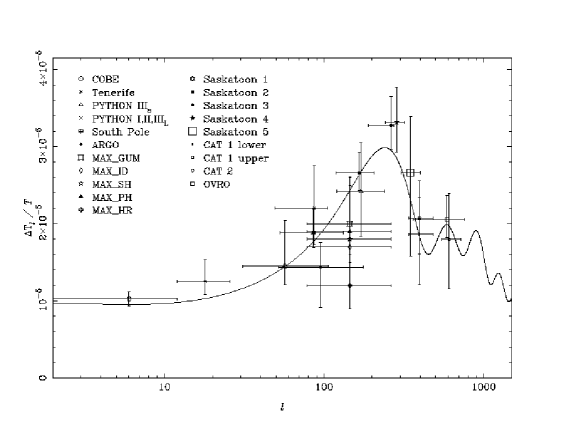
Figure 1: A compilation of CMB measurements and the ‘best fit’ universe based on the joint CMB+IRAS estimation, for parameters given in Table 1.

As in Hancock et al. (1998) we form a chi-squared $\chi^{2}({\vec{\alpha}}_{\rm cmb})$ statistic between the flat bandpowers $\Delta T_{l}$ (20 measurements) for a given set of parameter values $({\vec{\alpha}}_{\rm cmb})$. Since the CMB data points were chosen such that no two bandpower estimates come from experiments which observed overlapping patches of sky and had overlapping window functions, we may consider them as independent estimates of the CMB power spectrum. As the cosmic variance has already been taken into account in deriving the flat bandpower estimates, the likelihood function is given simply by ${\cal L}_{\rm cmb}\propto e^{-\chi^{2}/2}$. We assume that the Universe is spatially flat, and that there are no tensor contributions to the CMB power spectrum. We take the primordial scalar perturbations to be described by the Harrison-Zel’dovich power spectrum for which ${n_{\rm s}}=1$, and further assume that the optical depth to the last scattering surface is zero. The normalisation of the CMB power spectrum is determined by $Q$, which gives the strength of the quadrupole in $\mu K$. Hereafter ${\Omega_{\rm cdm}}$ and ${\Omega_{\rm b}}$ denote the density of the Universe in CDM and the baryons respectively, each in units of the critical density. Given that we assume a flat universe, but investigate models where ${\Omega_{\rm m}}\equiv({\Omega_{\rm cdm}}+{\Omega_{\rm b}})<1\$, the shortfall is made up through a non-zero cosmological constant $\Lambda$ such that ${\Omega_{\Lambda}}=1-{\Omega_{\rm m}}={{\Lambda}/({3{H_{0}^{2}}})}\$ . Furthermore, we restrict our attention to models that satisfy the nucleosynthesis constraint $\Omega_{b}h^{2}=0.024$ (Tytler et al. 1996). Thus we consider the reduced set of CMB parameters

$${\vec{\alpha}}_{\rm cmb}\equiv\{Q,h,{\Omega_{\rm cdm}}\}\ .$$ (1)

3 IRAS

We use the 1.2 Jy IRAS survey (Fisher et al. 1995), consisting of 5313 galaxies, covering 87.6% of the sky. Here we assume linear, scale-independent biasing, where ${b_{\rm iras}}$ measures the ratio between fluctuations in the IRAS galaxy distribution and the underlying mass density field:

$${\left({{\delta\rho}/{\rho}}\right)}_{\rm iras}={b_{\rm iras}}\,{\left({{\delta\rho}/{\rho}}\right)_{\rm m}}\ .$$ (2)

We note that biasing may be non-linear, stochastic, non local, scale dependent, epoch dependent and type dependent (e.g. Dekel & Lahav 1998, Tegmark & Peebles 1998, Blanton et al. 1998, and references therein). For a linear bias parameter, ${b_{\rm iras}}$, the velocity and density fields in linear theory are linked by a proportionality factor ${\beta_{\rm iras}}\equiv{{{\Omega_{\rm m}}^{0.6}}/{{b_{\rm iras}}}}$. Statistically, the fluctuations in the real-space galaxy distribution can be described by a power spectrum, ${P(k)}$, which is determined by the rms variance in the observed galaxy field, measured for an 8$\ {h^{-1}\rm Mpc}$ radius sphere (${\sigma_{8,{\rm iras}}}$) and a shape parameter (e.g. $\Gamma$ below). The observed ${\sigma_{8,{\rm iras}}}$ is related to the underlying ${\sigma_{8}}$ for mass through the bias parameter, such that ${\sigma_{8,{\rm iras}}}={b_{\rm iras}}\,{\sigma_{8}}$. We follow the spherical harmonic approach of Fisher, Scharf & Lahav (1994). The likelihood of the survey harmonics can be calculated as

$${\cal L}_{\rm iras}\propto{{\left|{\bf A}\right|}^{-{{1}\over{2}}}}\,{{\rm exp}^{\left({{-{{1}\over{2}}}\left[{{\vec{a}}^{\rm T}}\,{\bf A}^{-1}\,{\vec{a}}\right]}\right)}}\ .$$ (3)

Here $\vec{a}$ is the vector of observed harmonics for different radial shells ${\bf A}$ is the corresponding covariance matrix, which depends on the predicted harmonics (including shot noise). Note that the argument of the exponent in equation 3 is simply $(-\chi^{2}/2)$, and that here the normalisation of the likelihood function does depend on the free parameters (unlike in the CMB likelihood function). Since our analysis is valid only in the linear regime, we restrict the likelihood computation to $l_{\rm max}=10$ (corresponding to 120 degrees of freedom). The IRAS window functions are sensitive to scales $k\sim 0.01-0.1$. To summarize, the IRAS likelihood function has a parameter vector

$${\vec{\alpha}}_{\rm iras}\equiv\{{\beta_{\rm iras}},{\sigma_{8,{\rm iras}}},\Gamma\}\ .$$ (4)

4 Joint analysis CMB+IRAS

Given the large number of parameters available between the two models, it is important both to find links for joint optimisation, and to decide which parameters can be frozen. From section 3, we have six variables between the two models: {$Q$, ${h}$, ${\Omega_{\rm cdm}}$, ${\beta_{\rm iras}}$, ${\sigma_{8,{\rm iras}}}$, $\Gamma$}. These can be reduced further by expression in terms of core cosmological parameters. The IRAS normalisation can be calculated as ${\sigma_{8}}\equiv f({\Omega_{\rm m}},Q,\Gamma)$, while the CDM shape parameter $\Gamma$ depends on ${\Omega_{\rm m}}\,{h}$ and ${\Omega_{\rm b}}$ (Sugiyama 1995). On the other hand, ${\Omega_{\rm m}}={\Omega_{\rm cdm}}+{\Omega_{\rm b}}$, ${\beta_{\rm iras}}=\Omega_{\rm m}^{0.6}/{b_{\rm iras}}$, and ${\sigma_{8,{\rm iras}}}={\sigma_{8}}{b_{\rm iras}}$. Hence, the final, joint parameter space is

$${\vec{\alpha}}_{\rm joint}\equiv\{{h},Q,{\Omega_{\rm m}},{b_{\rm iras}}\}\ .$$ (5)

As the IRAS and CMB probe very different scales and hence are assumed to be uncorrelated, the joint likelihood is given by

$${\rm ln}\left({\cal L}_{\rm joint}\right)={\rm ln}\left({\cal L}_{\rm cmb}\right)+{\rm ln}\left({\cal L}_{\rm iras}\right)\ .$$ (6)

The joint likelihood (equation 6) was maximized with respect to the 4 free parameters (equation 5) and the best fit parameters are shown in Table 1.

Table 1. — Parameter values at the joint optimum. The 68% confidence limits are shown, calculated for each parameter by marginalising the likelihood over the other variables. ${\Omega_{\rm m}}$ $0.39$ $0$. $29$ $\,<\,$ ${\Omega_{\rm m}}$ $\,<\,$ $0$. $53$ $h$ $0.53$ $0$. $39$ $\,<\,$ $h$ $\,<\,$ $0$. $58$ $Q$ ($\mu$K) $16.95$ $15$. $34$ $\,<\,$ $Q$ $\,<\,$ $17$. $60$ ${b_{\rm iras}}$ $1.21$ $0$. $98$ $\,<\,$ ${b_{\rm iras}}$ $\,<\,$ $1$. $56$

It follows that $\Omega_{b}=0.085$, ${\sigma_{8}}=0.67$, $\sigma_{8,{\rm iras}}=0.81$, $\Gamma=0.15$, ${\beta_{\rm iras}}=0.47$ and the age of the Universe is $16.5$ Gyr. For this set of parameters, we find the values of the reduced $\chi^{2}$ for the IRAS and CMB data respectively to be 1.18 and 1.03, confirming that both data-sets agree well with the models used. Taking the CMB and IRAS data together the total reduced $\chi^{2}$ is 1.16. We note that our joint IRAS & CMB optimal values for $\sigma_{8,{\rm iras}},\beta_{{\rm iras}}$ and $\Gamma$ (Table 1) are in perfect agreement with the values derived from IRAS alone (Fisher et al. 1994, Fisher 1994). However at fixed $\sigma_{8,{\rm iras}}=0.69$ based on the IRAS correlation function Fisher et al. (1994) found a higher $\beta_{{\rm iras}}=0.94\pm 0.17$ and $\Gamma=0.17\pm 0.05(1-\sigma)$. To obtain 68 per cent confidence limits on each of the free parameters it is necessary to marginalise over the remaining free parameters. The marginalised distribution for each parameter is shown in Figure 2, in which the dashed vertical lines denote the 68% confidence limits quoted in Table 1.

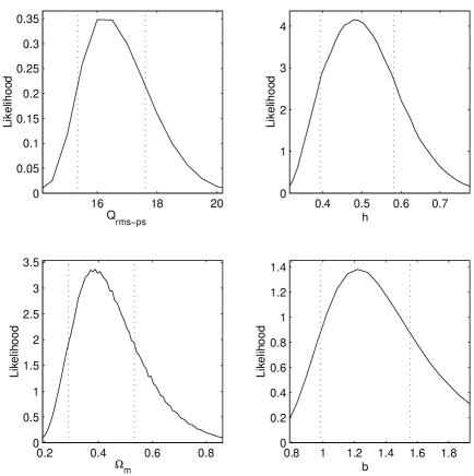
Figure 2: The one-dimensional marginalised probability distributions for each of the four parameters. The vertical dashed lines denote the 68% confidence limits. The horizontal plot limits are at the 99% confidence limits.

In addition we evaluated the covariance matrix at the joint optimum. The most strongly correlated parameters are ${\Omega_{\rm m}}$ and $h$, with (normalized) correlation coefficient of $(-0.82)$ .

5 The XRB

Although discovered in 1962, the origin of the X-ray Background (XRB) is still unknown, but is likely to be due to sources at high redshift (for a review see Fabian & Barcons 1992). Here we shall not attempt to speculate on the nature of the XRB sources. Instead, we utilise the XRB as a probe of the density fluctuations at high redshift. The XRB sources are probably located at redshift $z<5$, making them convenient tracers of the mass distribution on scales intermediate between those in the CMB as probed by COBE, and those probed by optical and IRAS redshift surveys (see Figure 3). The interpretation of the results depends somewhat on the nature of the X-ray sources and their evolution. The rms dipole and higher moments of spherical harmonics can be predicted (Lahav, Piran & Treyer 1997) in the framework of growth of structure by gravitational instability from initial density fluctuations. By comparing the predicted multipoles to those observed by HEAO1 (Treyer et al. 1998) we estimate the amplitude of fluctuations for an assumed shape of the density fluctuations (e.g. CDM models). Figure 3 shows the amplitude of fluctuations derived at the effective scale $\lambda\sim 600h^{-1}$ Mpc probed by the XRB. The observed fluctuations in the XRB are roughly as expected from interpolating between the local galaxy surveys and the COBE CMB experiment. The rms fluctuations ${{\delta\rho}\over{\rho}}$ on a scale of $\sim 600h^{-1}$Mpc are less than 0.2 %.

Figure 3: A compilation of rms density fluctuations, $({{\delta\rho}\over{\rho}})^{2}\sim k^{3}P(k)$, on different scales from various observations: a galaxy survey, the X-ray Background and Cosmic Microwave Background experiments. The crosses represent constraints from the XRB HEAO1 quadrupole (Lahav et al. 1997, Treyer et al. 1998). The top and bottom crosses are estimates of the amplitude of the power-spectrum at $k^{-1}\sim 600h^{-1}$ Mpc, assuming CDM power-spectra with shape parameters $\Gamma=0.2$ and $0.5$ respectively, and an Einstein-de Sitter universe. The fractional error on the XRB amplitudes (due to the shot-noise of the X-ray sources) is about 30%. The solid and dashed lines correspond to the standard CDM power-spectrum (with shape parameter $\Gamma=0.5$) and a ‘low-density’ CDM power-spectrum (with $\Gamma=0.2$), respectively, assuming $\sigma_{8}=1$ in both cases. The open squares at small scales are estimates of the power-spectrum from 3D inversion of the angular APM galaxy catalogue (Baugh & Efstathiou 1994). The elongated box at large scales represent the COBE 4-yr CMB measurement. The COBE box corresponds to a quadrupole Q=18.0 $\mu K$ for a Harrison-Zeldovich mass power-spectrum, via the Sachs-Wolfe effect, or $\sigma_{8}=1.4$ for a standard CDM model (Gawiser and Silk 1998).

5.1 Joint IRAS+XRB estimation

For simplicity we restricted the analysis to the standard CDM model (${\Omega_{\rm m}}=1,h=0.5$) with normalization $\sigma_{8}=0.7$. Here we assumed a revised ${\Omega_{\rm b}}h^{2}=0.019$ (Burles & Tytler 1998). As the sources of the XRB cover a wide range in redshift we assumed an epoch-dependent biasing of the form (Fry 1996):

$$b_{x}(z)=b_{x}(0)+z[b_{x}(0)-1]$$ (7)

and that the X-ray emissivity varies like $(1+z)^{2.6}$ out to $z_{max}=6.4$ (Treyer et al. 1998). In the likelihood analysis we used the HEAO1 data with a Galactic mask, and harmonics $1\leq l\leq 10$. We then maximized the joint likelihood IRAS+XRB (assumed to be uncorrelated) with respect to 2 free biasing parameters, and found at the ${b_{\rm iras}}=1.1$ and $b_{x}(0)=2.6$. The goodness-of-fit is $\chi^{2}_{iras}=1.22$ and $\chi^{2}_{xrb}=1.01$.

5.2 Joint IRAS+XRB+CMB estimation

We then added the CMB and solved for 3 free parameters: ${b_{\rm iras}}=0.7$, $b_{x}(0)=1.8$ and $\sigma_{8}=1.0$. While the $\chi^{2}$ for IRAS and XRB are acceptable, the CMB fit is very poor, $\chi^{2}_{cmb}=2.7$. Hence standard CDM cannot fit these 3 data sets simultaneously. We intend to generalise this analysis for other models.

6 Comparison with other studies

The results of the CMB+IRAS optimisation are in reasonable agreement with other current estimates. The relatively low value of ${\Omega_{\rm m}}\approx 0.4$ is close to that found by others (White et al. 1993, Bahcall et al. 1997), and is in line with recent supernovae results (Perlmutter et al. 1998). However, given the assumption of a flat universe, it requires a very high cosmological constant (${\Omega_{\Lambda}}=0.6$). Gravitational lensing measurements have constrained ${\Omega_{\Lambda}}<0.7$ (Kochanek 1996). Our value for the Hubble constant, ${h}=0.53$, agrees well with several other measurements (Sugiyama 1995, Lineweaver et al. 1997), but falls at the low end of the generally accepted range from local measurements (Freedman et al. 1998). Assuming the nucleosynthesis constraint $\Omega_{b}h^{2}=0.024$ the optimal baryon density is found to be ${\Omega_{\rm b}}=0.085$. Our value for the combination ${\sigma_{8}}{\Omega_{\rm m}}^{0.6}=0.38$ is lower than the one derived from measurements from the peculiar velocity field, $\sigma_{8}{\Omega_{\rm m}}^{0.6}\approx 0.8$ (Freudling et al. 1998). Our values are closer to the combination derived from cluster abundance $\sigma_{8}{\Omega_{\rm m}}^{0.5}\approx 0.5$ (Eke et al. 1998). Finally, for spatially-flat universes the time since the Big Bang for the values of our ${\Omega_{\rm m}}$ and $h$ at the joint optimum is $16.5$ Gyr. On the IRAS side, ${\beta_{\rm iras}}=0.47$ is in agreement with several other measurements (Willick et al. 1997), although there are other measurements which place ${\beta_{\rm iras}}$ much higher (Sigad et al. 1997). Finally, the IRAS mass-to-light bias is seen to be slightly greater than unity (${b_{\rm iras}}=1.2$), suggesting that the IRAS galaxies (mainly spirals) are reasonable (but not perfect) tracers of the underlying mass distribution. On the other hand, the XRB sources are strongly biased relative to the mass ($b_{x}(0)=2.6$).

7 Is the FRW Metric Valid on Large Scales ?

The Cosmological Principle was first adopted when observational cosmology was in its infancy; it was then little more than a conjecture. Observations could not then probe to significant redshifts, the ‘dark matter’ problem was not well-established and the CMB and the XRB were still unknown. If the Cosmological Principle turned out to be invalid then the consequences to our understanding of cosmology would be dramatic, for example the conventional way of interpreting the age of the universe, its geometry and matter content would have to be revised. Therefore it is important to revisit this underlying assumption in the light of new galaxy surveys and measurements of the XRB and CMB. The question of whether the universe is isotropic and homogeneous on large scales can also be phrased in terms of the fractal structure of the universe. A fractal is a geometric shape that is not homogeneous, yet preserves the property that each part is a reduced-scale version of the whole. If the matter in the universe were actually distributed like a pure fractal on all scales then the Cosmological Principle would be invalid, and the standard model in trouble. As shown in Figure 3 current data already strongly constrain any non-uniformities in the galaxy distribution (as well as the overall mass distribution) on scales $>300\,h^{-1}\,{\rm Mpc}$. If we count, for each galaxy, the number of galaxies within a distance $R$ from it, and call the average number obtained $N(<R)$, then the distribution is said to be a fractal of correlation dimension $D_{2}$ if $N(<R)\propto R^{D_{2}}$. Of course $D_{2}$ may be 3, in which case the distribution is homogeneous rather than fractal. In the pure fractal model this power law holds for all scales of $R$. The fractal proponents (Pietronero et al. 1997) have estimated $D_{2}\approx 2$ for all scales up to $\sim 1000\,h^{-1}\,{\rm Mpc}$, whereas other groups have obtained scale-dependent values (for review see Wu, Lahav & Rees 1998, and references therein). If we assume homogeneity on large scales, then we have a direct mapping between correlation function $\xi(r)$ (or the Power-spectrum) and $D_{2}$. For $\xi(r)\propto r^{-\gamma}$ it follows that $D_{2}=3-\gamma$ if $\xi\gg 1$, while if $\xi(r)=0$ then $D_{2}=3$. We note that it is inappropriate to quote a single crossover scale to homogeneity, for the transition is gradual. Direct estimates of $D_{2}$ are not possible for much larger scales, but we can calculate values of $D_{2}$ at the scales probed by the XRB and CMB by using CDM models normalised with the XRB and CMB as described above. The resulting values are consistent with $D_{2}=3$ to within $10^{-4}$ from the XRB on scales $\sim 500\,h^{-1}\,{\rm Mpc}$ and $2\times 10^{-5}$ from the CMB on $\sim 1000\,h^{-1}\,{\rm Mpc}$ (Wu et al. 1998). Isotropy does not imply homogeneity, but the near-isotropy of the CMB can be combined with the Copernican principle that we are not in a preferred position.

8 Discussion

The near future will see a dramatic increase in LSS data (e.g. the PSCZ, SDSS, 2dF and 6dF surveys) and detailed measurements of the CMB fluctuations on sub-degree scales (e.g. from the Planck Surveyor and MAP satellites). These will allow more accurate parameter estimation and exploration of a wider range of models. In particular we emphasise that the naive linear biasing should be generalised to more realistic scenarios. Other cosmological probes (e.g. Supernovae, clusters, peculiar velocities and radio sources) can be added to the analysis to set tighter constraints on the parameter space.

Acknowledgments

We thank M. Hobson, A. Lasenby, M. Rees, G. Rocha , C. Scharf, M. Treyer, M. Webster, and K. Wu for their contribution for the work presented here.

References

- [1] Bahcall N.A., Fan, X., & Cen, R. 1997, ApJ, 485, L53
- [2] Baugh C.M. & Efstathiou G., 1994, MNRAS, 267, 323
- [3] Blanton, M., Cen, R., Ostriker, J.P., & Strauss, M.A., 1998, astro-ph/9807029
- [4] Burles S. & Tytler, D., 1998, astro-ph/9803071
- [5] Dekel, A. & Lahav, O., submitted to ApJ, astro-ph/9806193
- [6] Eisenstein, D.J., Hu, W. & Tegmark, M., 1998, astro-ph/9807130
- [7] Eke, V.R., Cole, S., Frenk, C.S. & Henry, J.P. 1998, astro-ph/9802350
- [8] Fabian, A. C. & Barcons, X., 1992, ARAA, 30, 429
- [9] Fisher, K.B., in proceedings of ‘Cosmic Velocity Fields’, Paris, eds. Bouchet et al., pg. 177, Editions Frontieres
- [10] Fisher, K.B., Scharf, C.A. & Lahav, O., 1994, MNRAS, 266, 219
- [11] Fisher, K.B., Huchra, J.P., Strauss, M.A., Davis, M., Yahil A., & Schlegel D., 1995, ApJ, 100, 69
- [12] Freedman, W.L. et al., astro-ph/ 9801080
- [13] Freudling et al., 1998, submitted to ApJ
- [14] Fry, J. 1996, ApJ Lett, 461, L65
- [15] Gawiser E., & Silk J., 1998, Science, 280, 1405
- [16] Hancock S., Rocha G., Lasenby A.N., & Gutierrez C.M., 1998, MNRAS, 294, L1
- [17] Kochanek C.S., 1996, ApJ, 466, 638
- [18] Lahav O., Piran T. & Treyer M.A., 1997, MNRAS, 284, 499
- [19] Lineweaver C.H., Barbosa D., Blanchard A. & Bartlett J.G., 1997, Astron. & Astrophy., 322, 365
- [20] Perlmutter S., et al. , 1998, Nature, 391, 51
- [21] Pietronero, L., Montuori M., & Sylos-Labini, F., 1997, in Critical Dialogues in Cosmology, ed. N. Turok, astro-ph/9611197.
- [22] Sigad Y., Dekel A., Strauss M.A. & Yahil A., 1998, 495, 516
- [23] Sugiyama N., 1995, ApJ Supp., 100, 281
- [24] Tegmark, M., & Peebles, P.J.E. 1998, astro-ph/9804067
- [25] Treyer, M., Scharf, C., Lahav, O., Jahoda, K., Boldt, E. & Piran, T., 1998, ApJ, in press, astro-ph/9801293.
- [26] Tytler D., Fan X.M. & Burles S., 1996, Nature, 381, 207
- [27] Webster, M., Bridle, S.L., Hobson, M.P., Lasenby, A.N., Lahav, O., & Rocha, G. 1998, ApJ Lett, submitted , astro-ph/9802109.
- [28] White, S.D. M., Navarro, J.F., Evrard, A.E. & Frenk, C.S., 1993, Nature, 366, 429
- [29] Willick J.A., Strauss M.A., Dekel A. & Kolatt T., 1997, ApJ, 486, 629
- [30] Wu, K.K.S., Lahav, O. & Rees, M.J., 1998, Nature, accepted, astro-ph/9804062.