Evidence for Scale-Scale Correlations in the Cosmic Microwave Background Radiation

Abstract

We perform a discrete wavelet analysis of the COBE-DMR 4yr sky maps and find a significant scale-scale correlation on angular scales from about 11 to 22 degrees, only in the DMR face centered on the North Galactic Pole. This non-Gaussian signature does not arise either from the known foregrounds or the correlated noise maps, nor is it consistent with upper limits on the residual systematic errors in the DMR maps. Either the scale-scale correlations are caused by an unknown foreground contaminate or systematic errors on angular scales as large as 22 degrees, or the standard inflation plus cold dark matter paradigm is ruled out at the $>99\%$ confidence level.

Most attempts at quantifying the non-Gaussianity in the cosmic microwave background radiation are motivated by the belief that non-Gaussianity can distinguish inflationary models of structure formation from topological models. While standard inflation predicts a Gaussian distribution of anisotropies [1], spontaneous symmetry breaking produces topological defects whose networks create non-Gaussian patterns on the microwave background radiation on small scales[2]. Minute non-Gaussian features can however be generated by gravitational waves [3] or by the Rees-Sciama [4] and Sunyaev-Zeldovich effects.

It is generally held that cosmic gravitational clustering can be roughly described by three régimes: linear, quasi-linear, and fully developed nonlinear clustering. Whilst quasi-linear and non-linear clustering induce non-Gaussian distribution functions, if the initial density perturbations are Gaussian, scale-scale correlations and other non-Gaussian features of the density field can not be generated during the linear régime. Hence the linear régime is best suited to study the primordial non-Gaussian fluctuations. Since the amplitudes of the cosmic temperature fluctuations revealed by COBE are as small as $\Delta T/T\simeq 10^{-5}$, the gravitational clustering should remain in the linear régime on scales larger than about 30 $h^{-1}$ Mpc and at redshifts higher than 2. Current limits on non-Gaussianity from galaxy surveys probe redshifts smaller than about 1 [5]. Interestingly, at redshifts between 2 and 3, and scales on the order of 40 to 80 $h^{-1}$ Mpc, there are positive detections of scale-scale correlations in the distribution of Ly$\alpha$ absorption lines in quasar spectra [6]. These clouds are likely to be pre-collapsed and continuously distributed intergalactic gas clouds, and are therefore fair tracers of the cosmic density field, especially on large scales [7]. This may indicate that the primordial fluctuations are scale-scale correlated.

While on small angular scales ($\ell\simeq 150$) there may be some indications of non-Gaussianity [8], studies by traditional non-Gaussian detectors have concluded that there is no evidence of non-Gaussianity in the cosmic temperature fluctuations on large scales [9]. (See however [10].) This does not rule out the existence of scale-scale correlations. Because each non-Gaussian feature is non-Gaussian in its own way, there is no single statistical indicator for the existence of non-Gaussianity in data. For instance, there are models of scale-scale coupling which lead to a density field with a Poisson distribution in its one-point distribution function, but that are highly scale-scale correlated [11]. In this case, all statistics based on the one-point functions will fail to detect the scale-scale correlations, that is, they will miss the non-Gaussianity. As yet, the scale-scale correlations of the cosmic temperature fluctuations have not been searched for in any available data set. It is the intent of this Letter to probe for the scale-scale correlations in the COBE-DMR 4-year sky maps, and, as an example, show that this measure is effective in testing models of the initial density perturbations. In contrast with other techniques, such as the bispectrum, [12], higher order cumulants [13], Minkowski functionals [14], or double Fourier analysis [15], scale-scale correlations are localized, and can localize the areas on the sky where the signal comes from, and with a resolution that depends on the scale considered.

The scale-scale correlations are conveniently described by the discrete wavelet transform (DWT) [6, 16]. Considering a 2-dimensional temperature (or density) field $T({\bf x})$, where ${\bf x}=(x_{1},x_{2})$, such that $0\leq x_{1},x_{2}\leq L$, the DWT scale-space decomposition of the contrast $\Delta T({\bf x})/T$ is

$$\frac{\Delta T}{T}=\sum_{j_{1}=0}^{J_{1}-1}\sum_{j_{2}=0}^{J_{2}-1}\sum_{l_{1}=0}^{2^{j_{1}}-1}\sum_{l_{2}=0}^{2^{j_{2}}-1}\tilde{\epsilon}_{j_{1},j_{2};l_{1},l_{2}}\psi_{j_{1},j_{2};l_{1},l_{2}}({\bf x}),$$ (1)

where $\psi_{j_{1},j_{2};l_{1},l_{2}}({\bf x})$ ($j_{1},j_{2}=0,1,2..$ and $l_{1}=0,1...2^{j_{1}}-1$, $l_{2}=0,1...2^{j_{1}}-1$) are the complete and orthogonal wavelet basis [17]. The indexes $(j_{1},j_{2})$ and $(l_{1},l_{2})$ denote the scale $(L/2^{j_{1}},L/2^{j_{2}})$ and position $(Ll_{1}/2^{j_{1}},Ll_{2}/2^{j_{2}})$ in phase space and $J_{1}$ and $J_{2}$ are the smallest scales possible (i.e., one pixel). The wavelet basis function, $\psi_{j_{1},j_{2};l_{1},l_{2}}({\bf x})$, is localized at the phase space point $(j_{1},j_{2};l_{1},l_{2})$ and the wavelet coefficients $\tilde{\epsilon}_{j_{1},j_{2};l_{1},l_{2}}$ measure the 2-D perturbations at the phase space point $(j_{1},j_{2};l_{1},l_{2})$. To be specific, we will use the Daubechies 4 wavelet in this paper, although the results are not affected by this choice so long as a compactly supported wavelet basis is used.

To measure correlations between scales $(j,j)$ and $(j+1,j+1)$, we define

$$C^{p,p}_{j}=\frac{2^{2(j+1)}\sum_{\bf{l}=0}^{2^{j+1}-1}\tilde{\epsilon}^{p}_{j;{\bf[l/2]}}\;\tilde{\epsilon}^{p}_{j+1;{\bf l}}}{\sum\tilde{\epsilon}^{p}_{j,{\bf[l/2]}}\sum\tilde{\epsilon}^{p}_{j+1;{\bf l}}}$$ (2)

where $p$ is an even integer, ${\bf l}\equiv(l_{1},l_{2})$, and the [  ]’s denote the integer part of the quantity. Because $Ll/2^{j}=L2l/2^{j+1}$, the position $l$ at scale $j$ is the same as the positions $2l$ and $2l+1$ at scale $j+1$. Therefore, $C_{j}^{p,p}$ measures the correlation between scales at the same physical point. For Gaussian fields, $C_{j}^{p,p}=1$. $C_{j}^{p,p}>1$ corresponds to a positive scale-scale correlation, and $C_{j}^{p,p}<1$ to the negative case. One can also show that a $C_{j}^{p,p}>1$ field cannot be produced by a $C_{j}^{p,p}<1$ distribution in a Gaussian background.

It is also possible to define the more “standard” non-Gaussian measures with the wavelet coefficients. Namely we define the third and fourth order cumulants as

$$S_{j}\equiv\frac{1}{(M_{j}^{2})^{3/2}}M^{3}_{j},\quad\quad K_{j}\equiv\frac{1}{(M_{j}^{2})^{2}}M^{4}_{j}-3,\quad\quad\quad\quad{\rm where}\quad\quad M^{n}_{j}\equiv\frac{1}{2^{2j}}\sum_{l_{1},l_{2}=0}^{2^{j}-1}(\tilde{\epsilon}_{j,j:l_{1},l_{2}}-\overline{\tilde{\epsilon}_{j,j;l_{1},l_{2}}})^{n},$$ (3)

and $\overline{\tilde{\epsilon}_{j,j;l_{1},l_{2}}}$ is the ensemble average (simulated samples) or the average over $(l_{1},l_{2})$ (real data).

The COBE-DMR data is formatted such that the entire sky is projected onto a cube with each of its 6 faces pixelized into $2^{10}$ approximately equal-area pixels. Although one could think of performing a spherical wavelet analysis directly on the sky, the current format is ideal for a direct 2-D DWT analysis. The pixels of each face can be labeled by $(j_{1},j_{2})$ with $0\leq j_{1},j_{2}\leq 5$, and $(l_{1},l_{2})$ with $0\leq l_{1}\leq 2^{j_{1}}$ and $0\leq l_{2}\leq 2^{j_{2}}$. The scale $j$ corresponds to angular scale $2.8\times 2^{5-j}$ degrees. In this way, one can analyze each face individually. This is important, as we can reduce the influence of the galactic foreground contamination by selecting the faces in the direction of galactic poles. The galactic plane stretches across Faces 1 - 4 (in galactic coordinates) of the projected cube, while Faces 0 and 5 are relatively free of galactic interference. We will concentrate on these two faces since the standard galactic cut at $|b|$ = 20 degrees implies that the other faces will be significantly contaminated.

Before attempting to measure the non-Gaussianity in the DMR maps, we should test for possible contamination due to various kinds of noise. A typical example of non-Gaussianity caused by noise is Poissonian noise. Fortunately, this type of non-Gaussianity can be properly handled by the higher order DWT cumulant spectra [16]. To quantify any non-Gaussianity due to DMR noise, we generate 1000 realizations of the temperature maps for a typical CDM model with parameters $\Omega_{0}=1$, $h=0.5$, and $\Omega_{b}=0.05$ and generate the appropriate sky maps at the DMR resolution [18]. To these maps, we linearly add noise to each pixel by drawing from a Gaussian distribution with the pixel dependent variance given by the two different foreground removal techniques, DCMB and DSMB (see [19] for details.)

Previous non-Gaussian studies using a genus method and other statistics, have found the four year DMR data to be consistent with a Gaussian field [9]. The evaluation of the genus at different smoothing angles is similar to the DWT scale decomposition which is also based on smoothing on various angular scales and suggests that the DWT cumulant spectra should give similar results. The results for $S_{j}$ and $K_{j}$ of the COBE-DMR foreground removed maps and the CDM model are shown in Fig. 1. Using the 1000 realizations of the CDM model, we construct the probability distribution for both $S_{j}$ and $K_{j}$. Fig. 1 gives the most probable values of $S_{j}$ and $K_{j}$ for the CDM model with the error bars corresponding to the 95% probability of drawing $S_{j}$, $K_{j}$ from the CDM model. Fig. 1 also shows that $S_{j}$ and $K_{j}$ for the DCMB and DSMB data are safely within the 95% range. Therefore, one can conclude that no significant non-Gaussianity can be identified from the third and fourth order cumulants. This result is consistent with the genus results. Note that contrary to previous studies, we can study the six faces of the cube separately. Fig. 1 shows that both $S_{j}$ and $K_{j}$ are isotropic with respect to the face 0 and 5.

We can now proceed to the scale-scale correlations. We list the most probable values of $C_{j}^{2,2}$ for the CDM+DSMB maps in Table 1. Similar results are obtained for the CDM+DCMB maps. Because the CDM model is a Gaussian model, all $C_{j}^{2,2}$ are about equal to 1 as expected. At any scale $j$, $C_{j}^{2,2}$ is about the same for face 0 and 5. Therefore, the noise from the two foreground removed DMR maps does not cause significant spurious scale-scale correlations and are thus suitable for a scale-scale correlation analysis. At the very least the sample is good for a comparison between observed scale-scale correlations with the CDM model.

The results for $C_{j}^{(2,2)}$ for the COBE-DMR foreground removed maps are plotted in Fig. 2 and tabulated in Table 1. The behavior of $C_{1}^{(2,2)}$ is markedly different from $S_{j}$, $K_{j}$, or the CDM+DSMB results. First, $C_{1}^{(2,2)}$ for face 0 cannot be drawn from the CDM model with a probability greater than 99%. Second, $C_{1}^{(2,2)}$ is not isotropic, showing a difference between faces 0 and 5. The DCMB maps show the same behavior.

$C_{1}^{(2,2)}$ describes the correlation between perturbations on angular scales of $\simeq 22$ and $\simeq 11$ degrees, which corresponds to comoving scales larger than about 100 $h^{-1}$ Mpc. Because the wavelets are orthogonal, $C_{1}^{(2,2)}$ cannot be changed by adding any abnormal process on angular scales less than $\simeq$ 10 degrees. The “surprisingly” large value for $C_{1}^{(2,2)}$ cannot be explained by any non-Gaussian process on small scales. We have shown that the errors of the foreground removed DMR maps cannot contribute to $C_{1}^{(2,2)}$.

We also checked for possible contributions to the non-Gaussianity from systematics by doing a similar analysis on the systematic error maps. It is unlikely that the detected non-Gaussianity comes from the systematics since the non-Gaussianity is on the order of $\simeq 10^{-5}$ K, while the contribution to the anisotropy from the systematics is estimated to be on order $\simeq 10^{-6}$ K [20]. The analysis of the combined systematic error maps confirms that $C_{j}^{2,2}$ is solidly in the Gaussian régime, i.e., $C_{1}^{2,2}=1.247\pm 0.375$. Moreover, these angular scales are larger than the resolution of the DMR instrument. Therefore, unless there are very local foreground contaminations which are overlooked by the two foreground removal methods, the high value for and the anisotropy in $C_{1}^{(2,2)}$ is cosmological.

To check if there could be large-scale foreground correlations overlooked by the COBE-DMR subtraction technique, we performed the same analysis on the dust maps generated by a careful combination of IRAS and DIRBE data [21]. Depending on the method used to obtain an averaged value for the color excess E(B-V) on a DMR pixel, the $C_{1}^{2,2}$ values range from $0.572\pm 0.747$ to $0.630\pm 0.617$. Although these maps show small-scale structure, when averaged over scales larger than the DMR pixels (2.8 degrees) any non-Gaussian fluctuation disappears. In addition we checked the possibility that the non-Gaussianity was due to anisotropies in the synchrotron emission by analysing an all-sky map at 408 MHz [23]. A visual inspection of this map shows a structure extending from the galactic plane on to the North Galactic Pole. However, using a map projected in the same way as the DMR maps we obtain $C_{1}^{2,2}=0.069$, which is much less than the value $C_{1}^{2,2}=1.008\pm 0.342$ obtained by 1000 bootstrap random realizations. As mentioned above, $C_{j}^{2,2}>1$ cannot come from a superposition of a distribution with $C_{j}^{2,2}<1$ in a Gaussian background. Thus the scale-scale correlation detected in the COBE-DMR data is not a result of this signal. Additionally, none of the individual frequency maps nor a linear combination consisting of the 53 GHz and 90 GHz frequencies maps show $C_{1}^{2,2}>1.5$. Since these maps do not contain the foreground subtractions, this result implies that if the cause of the signal in face 0 is foreground, it is incoherent.

As a final check, we also looked at the correlated noise maps in COBE-DMR [22]. The individual correlated noise maps of the frequencies were checked for scale-scale correlations and once again, $C_{1}^{2,2}$ was solidly in the Gaussian régime with $C_{1}^{2,2}=1.007\pm 0.440$ for the 31 GHz channel, $C_{1}^{2,2}=0.896\pm 0.308$ for the 53 GHz channel, and $C_{1}^{2,2}=0.935\pm 0.310$ at 90 GHz.

If indeed we have eliminated all non-cosmological sources that could account for this signature and if the signal is not just a statistical fluke (since there is still a 1% chance of this occuring), then the only conclusion left is that the correlation is cosmological in origin. Whether this signature arises from previously proposed sources of non-Gaussianity, such as cosmic strings, large spots, matter-antimatter domain interfaces, etc., remains to be determined.

Recall that the COBE-DMR data tolerate almost all popular models of primordial density perturbations in terms of the second order statistics. Generally, the data are only able to discriminate among the power spectra of these models with less than 2-$\sigma$ confidence levels [24]. The scale-scale correlation detected in the 4-year COBE-DMR data either gives a rather high confidence of ruling out the CDM model or evidence for the existence of unknown local foreground contamination on angular scales as large as $\simeq$ 10 – 20 degrees. Obviously, if either of these implications are correct, two important conclusions can be inferred: 1.) the inflation plus cold dark matter model with standard cosmological parameters appears to be ruled out at the $>99\%$ confidence; 2.) the COBE-DMR temperature maps are contaminated on large angular scales at levels larger than previously thought. Whether COBE determined cosmological parameters, such as the quadrupole of temperature fluctuations, may also be contaminated remains to be seen.

We are very grateful to Al Kogut for providing the systematic error and 408 MHz maps used in the analysis.

TABLE I.: Measured $C_{j}^{2,2}$ coefficients.

FACE 0				FACE 5
$j$	DMR	CDM+DSMB	95% Confidence Levels	DMR	CDM+DSMB	95% Confidence Levels
1	2.091	1.004	(0.376 – 1.587)	0.730	1.008	(0.492 – 1.761)
2	0.984	1.035	(0.601 – 1.513)	1.300	1.022	(0.688 – 1.572)
3	1.041	1.032	(0.791 – 1.294)	1.172	1.026	(0.832 – 1.358)

 

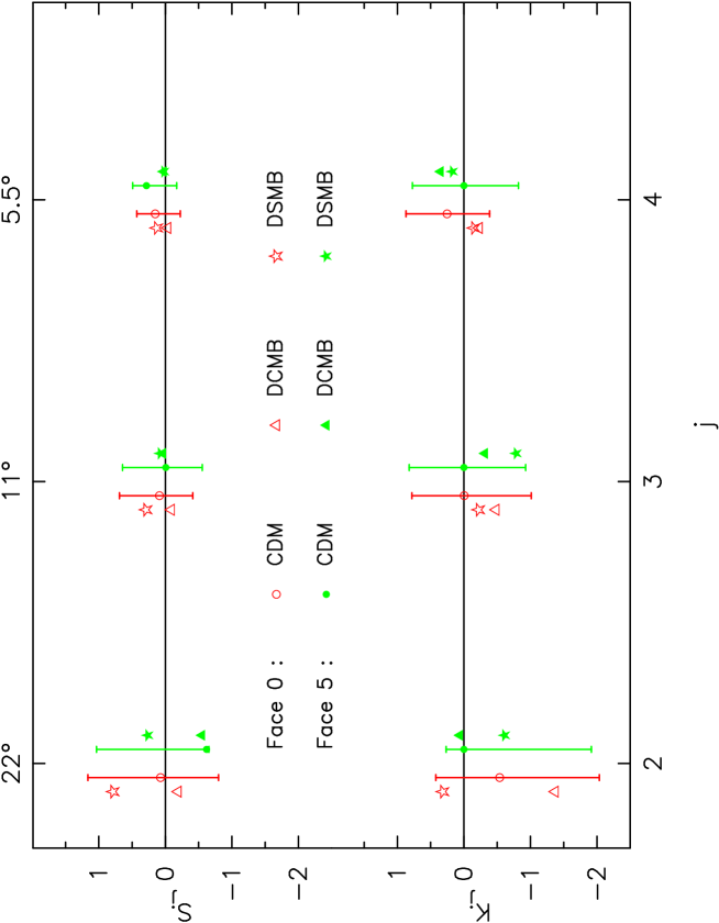
FIG. 1.: $S_{j}$ (top) and $K_{j}$ (bottom) for faces 0 and 5 of the DMR data and the CDM simulations.

 

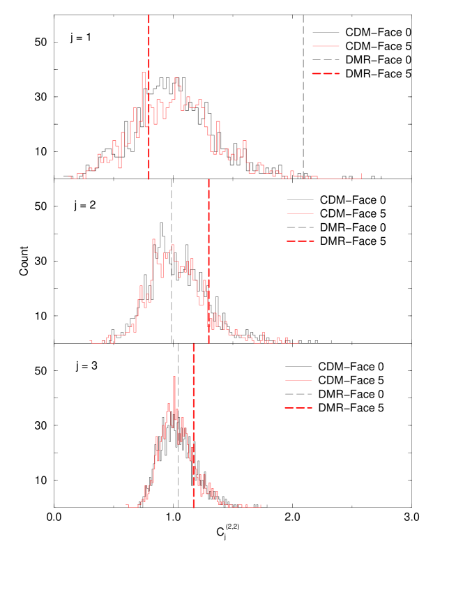
FIG. 2.: $C_{j}^{(2,2)}$ for faces 0 and 5 of the DMR data and the CDM simulations.

REFERENCES

- [1] A.H. Guth, Phys Rev D, 23, 347 (1981); A. Linde Phys. Lett. B, 108, 389 (1982); J.M. Bardeen, et al, Phys. Rev. D, 28, 679 (1983); A. Liddle & D. Lyth Phys. Rep. 231, 1 (1993).
- [2] T.W. Kibble Phys. Rep. 67 183 (1980); A. Vilenkin Phys. Rep. 121, 263 (1985); F.R. Bouchet, et al, Nature 335, 410 (1988); N. Turok & D.N. Spergel Phys. Rev. Lett., 66, 3093 (1991).
- [3] S. Bharadwaj, D. Munshi & T. Souradeep Phys. Rev. D56, 4503 (1997).
- [4] S. Mollerach et al. Astrophys. J. 453, 1 (1995).
- [5] A.J. Stirling & J.A. Peacock MNRAS 283 L99 (1996).
- [6] J. Pando, P. Lipa, M. Greiner, & L.Z. Fang, Astrophys. J. 496, 9, (1998).
- [7] H.G. Bi & A.F. Davidsen, Astrophys. J. 497, 523, (1997).
- [8] E. Gaztañaga, P. Fosalba & E. Elizalde MNRAS 295 L35 (1998).
- [9] A. Kogut et al. Astrophys. J. 464, L29, (1996)..
- [10] P.G. Ferreira, J. Magueijo & K.M. Górski Astrophys. J., 503, L1 (1998).
- [11] M. Greiner, P. Lipa & P. Carruthers, Phys. Rev. E51, 1948, (1995).
- [12] X. Luo Astrophys. J. 427 L71 (1994); A.F. Heavens MNRAS,299, 805 (1998).
- [13] P.G. Ferreira, J. Magueijo & J. Silk Phys. Rev. D. 56 4592 (1997).
- [14] S. Winitzki & A Kosowsky New Astron. 3 75 (1997)
- [15] A. Lewin, A. Albrecht & J. Magueijo astro-ph 9804283 (1998).
- [16] L.Z. Fang & J.Pando, in The 5th Current Topics of Astrofundamental Physics, eds. N.Sanchez & A.Zichichi, World Scientific, Singapore, 616, (1997).
- [17] I. Daubechies, Ten Lectures on Wavelets, SIAM, (1992); M. Holschneider, Wavelets : an analysis tool, Oxford Univ. Press, (1990); S. Mallat, A wavelet tour of signal processing, Academic Press, (1998).
- [18] U. Seljak & M. Zaldarriaga Astrophys. J., 469, 437 (1996); F. Muciaccia, et al, Astrophys. J., 488, L63 (1997).
- [19] C.L. Bennett et al, Astrophys. J., 396, L7, (1992); C.L. Bennett et al, Astrophys. J., 436, 423, (1994).
- [20] A. Kogut et at. Astrophys. J., 470, 653, (1996).
- [21] D. Schlegel, D. Finkbeiner & M. Davis, Astrophys. J, 500, 525,(1998).
- [22] C.H. Lineweaver, et al, Astrophys. J. 436, 452 (1994).
- [23] C. G. T. Haslam, C. J. Salter, H. Stoffel, & W. E. Wilson, A&AS, 47, 1 (1982).
- [24] Y.P. Jing & L.Z. Fang, Phys. Rev. Lett., 73, 1882, (1994); A. Berera, L.Z. Fang & G. Hinshaw, Phys. Rev., D57, 2207, (1998).