Cosmology with the Lyman-alpha Forest

Abstract

ABSTRACT. We outline the physical picture of the high-redshift Ly$\alpha$ forest that has emerged from cosmological simulations, discuss statistical characteristics of the forest that can be used to test theories of structure formation, present a preliminary comparison between simulation predictions and measurements from a sample of 28 Keck HIRES QSO spectra, and summarize the results of a recent determination of the linear mass power spectrum $P(k)$ at $z=2.5$ from a sample of 19 moderate resolution QSO spectra. The physical picture is simple if each QSO spectrum is viewed as a continuous non-linear map of the line-of-sight density field rather than a collection of discrete absorption lines. To a good approximation, the relation between Ly$\alpha$ optical depth and mass overdensity is $\tau=A({\rho/{\overline{\rho}}})^{1.6}$. The constant $A$ depends on poorly known physical parameters, but for a specified cosmological model its value can be calibrated using the mean flux decrement $\langle D\rangle\equiv\langle 1-e^{-\tau}\rangle$, leaving all other statistical properties of the forest as independent model predictions. The distribution of flux decrements is closely tied to the probability distribution function (PDF) of the underlying mass distribution, and hence to the amplitude and PDF (Gaussian or non-Gaussian) of the primordial density fluctuations. The threshold crossing frequency, analogous to the 3-d genus curve, responds to the shape and amplitude of the primordial $P(k)$ and to the values of $\Omega_{0}$ and $\Omega_{\Lambda}$. The predictions of open CDM and $\Lambda$CDM models agree well with the measured flux decrement distribution at smoothing lengths of $25{\rm\;km\;s^{-1}}$ and $100{\rm\;km\;s^{-1}}$ and with the threshold crossing frequency at $100{\rm\;km\;s^{-1}}$. Discrepancy with the observed threshold crossing frequency at $25{\rm\;km\;s^{-1}}$ smoothing may reflect the combined effects of noise in the data and limited mass resolution of the simulations. The moderate resolution spectra yield the slope and amplitude of the linear mass $P(k)$ at $2\pi/k\sim 700{\rm\;km\;s^{-1}}$. The slope, never previously measured on these scales, agrees with the predictions of inflation+CDM models. Combining the amplitude with COBE normalization imposes a constraint on these models of the form $\Omega_{0}h^{\alpha}n^{\beta}\Omega_{\rm b}^{\gamma}={\rm constant}.$ Assuming Gaussian primordial fluctuations and a power spectrum shape parameter $\Gamma\approx 0.2$, consistency of the measured $P(k)$ with the observed cluster mass function at $z=0$ requires $\Omega_{0}=0.46^{+0.12}_{-0.10}$ for $\Omega_{\Lambda}=0$ and $\Omega_{0}=0.34^{+0.13}_{-0.09}$ for $\Omega_{\Lambda}=1-\Omega_{0}$ ($1\sigma$ errors).

ABSTRACT. We outline the physical picture of the high-redshift Ly$\alpha$ forest that has emerged from cosmological simulations, discuss statistical characteristics of the forest that can be used to test theories of structure formation, present a preliminary comparison between simulation predictions and measurements from a sample of 28 Keck HIRES QSO spectra, and summarize the results of a recent determination of the linear mass power spectrum $P(k)$ at $z=2.5$ from a sample of 19 moderate resolution QSO spectra. The physical picture is simple if each QSO spectrum is viewed as a continuous non-linear map of the line-of-sight density field rather than a collection of discrete absorption lines. To a good approximation, the relation between Ly$\alpha$ optical depth and mass overdensity is $\tau=A({\rho/{\overline{\rho}}})^{1.6}$. The constant $A$ depends on poorly known physical parameters, but for a specified cosmological model its value can be calibrated using the mean flux decrement $\langle D\rangle\equiv\langle 1-e^{-\tau}\rangle$, leaving all other statistical properties of the forest as independent model predictions. The distribution of flux decrements is closely tied to the probability distribution function (PDF) of the underlying mass distribution, and hence to the amplitude and PDF (Gaussian or non-Gaussian) of the primordial density fluctuations. The threshold crossing frequency, analogous to the 3-d genus curve, responds to the shape and amplitude of the primordial $P(k)$ and to the values of $\Omega_{0}$ and $\Omega_{\Lambda}$. The predictions of open CDM and $\Lambda$CDM models agree well with the measured flux decrement distribution at smoothing lengths of $25{\rm\;km\;s^{-1}}$ and $100{\rm\;km\;s^{-1}}$ and with the threshold crossing frequency at $100{\rm\;km\;s^{-1}}$. Discrepancy with the observed threshold crossing frequency at $25{\rm\;km\;s^{-1}}$ smoothing may reflect the combined effects of noise in the data and limited mass resolution of the simulations. The moderate resolution spectra yield the slope and amplitude of the linear mass $P(k)$ at $2\pi/k\sim 700{\rm\;km\;s^{-1}}$. The slope, never previously measured on these scales, agrees with the predictions of inflation+CDM models. Combining the amplitude with COBE normalization imposes a constraint on these models of the form $\Omega_{0}h^{\alpha}n^{\beta}\Omega_{\rm b}^{\gamma}={\rm constant}.$ Assuming Gaussian primordial fluctuations and a power spectrum shape parameter $\Gamma\approx 0.2$, consistency of the measured $P(k)$ with the observed cluster mass function at $z=0$ requires $\Omega_{0}=0.46^{+0.12}_{-0.10}$ for $\Omega_{\Lambda}=0$ and $\Omega_{0}=0.34^{+0.13}_{-0.09}$ for $\Omega_{\Lambda}=1-\Omega_{0}$ ($1\sigma$ errors).

1 Introduction

For decades, the study of large scale structure was virtually synonymous with the study of galaxy clustering. The 1980s and 1990s have seen spectacular improvements in galaxy redshift and peculiar velocity data, many of them documented at this meeting. At this point, our ability to draw cosmological conclusions from these data is often limited less by their statistical uncertainties than by our limited understanding of the complex physics of galaxy formation. CMB anisotropy measurements have been enormously influential because their underlying physics is simpler, allowing a straightforward connection between theory and observation. However, even the ambitious CMB experiments now underway will yield only a particular projection of the evolution of cosmic structure, mostly concentrated at $z\sim 1000$. Other measures that probe 3-dimensional structure at later redshifts are needed to complement these experiments. The success of hydrodynamic cosmological simulations in explaining the basic properties of the Ly$\alpha$ forest (Cen et al. 1994; Zhang, Anninos, & Norman 1995; Hernquist et al. 1996; Wadsley & Bond 1996; Theuns et al. 1998) has opened up a new testing ground for cosmological theories. Ground-based observations yield superb data on the Ly$\alpha$ forest at $z\sim 2-4$, and HST spectra provide lower resolution measurements at $z\sim 0-2$. Equally important, the simulations lead to a simple physical picture of the Ly$\alpha$ forest, one that is well approximated by semi-analytic models that were to a significant extent developed prior to and independent of the simulations (McGill 1990; Bi 1993; Bi, Ge, & Fang 1995; Bi & Davidsen 1997; Hui, Gnedin, & Zhang 1997). We will briefly describe this physical picture in the next section (more extended discussions along these lines appear in Weinberg et al. 1997 and Weinberg, Katz, & Hernquist 1998, hereafter WKH). We will then discuss the physical significance of two statistics that can be used to test cosmological models against Ly$\alpha$ forest data and present a preliminary comparison between predictions from smoothed particle hydrodynamics (SPH) simulations and measurements from a sample of Keck HIRES spectra. We conclude with a discussion of a recent determination of the mass power spectrum at $z=2.5$ and its implications for the value of $\Omega_{0}$ and the parameters of CDM models.

2 Physics of the Ly$\alpha$ Forest

Figure 1: A test of the Fluctuating Gunn-Peterson Approximation on artificial spectra extracted from an SPH simulation of standard CDM in real space (right) and redshift space (left), at $z=3$. Points show the relation between Ly$\alpha$ optical depth and gas overdensity in the simulated spectra, pixel by pixel. Diagonal lines show the prediction of equation (1).

In hydrodynamic simulations of high redshift structure ($z\sim 2-5$), the Ly$\alpha$ forest is produced mainly by gas with overdensity ${\rho/{\overline{\rho}}}\mathrel{\hbox{\hbox to0.0pt{\hbox{\lower 4.0pt\hbox{$\sim$}}\hss}\hbox{$<$}}}10$. Most of this gas is unshocked, and the competition between photoionization heating and adiabatic cooling leads to a tight relation between $\rho$ and $T$ that is well approximated by a power law, $T=T_{0}({\rho/{\overline{\rho}}})^{\alpha}$. The values of $T_{0}$ and $\alpha$ depend on the reionization history of the universe and on the spectral shape of the UV background; they typically lie in the ranges $4000\,{\rm K}\mathrel{\hbox{\hbox to0.0pt{\hbox{\lower 4.0pt\hbox{$\sim$}}\hss}\hbox{$<$}}}T_{0}\mathrel{\hbox{\hbox to0.0pt{\hbox{\lower 4.0pt\hbox{$\sim$}}\hss}\hbox{$<$}}}10,000\,{\rm K}$ and $0.3\mathrel{\hbox{\hbox to0.0pt{\hbox{\lower 4.0pt\hbox{$\sim$}}\hss}\hbox{$<$}}}\alpha\mathrel{\hbox{\hbox to0.0pt{\hbox{\lower 4.0pt\hbox{$\sim$}}\hss}\hbox{$<$}}}0.6$ (Hui & Gnedin 1997). The optical depth for Ly$\alpha$ absorption is proportional to the neutral hydrogen density, which for gas in photoionization equilibrium near $10^{4}{\rm K}$ is proportional to $\rho^{2}T^{-0.7}/\Gamma_{\rm HI}$, where $\Gamma_{\rm HI}$ is the HI photoionization rate and the $T^{-0.7}$ factor accounts for the temperature dependence of the recombination rate. The combination of photoionization equilibrium and the $\rho-T$ relation therefore leads to a power law relation between optical depth, $\tau$, and gas overdensity ${\rho/{\overline{\rho}}}$,

$$\tau = A({\rho/{\overline{\rho}}})^{\beta}\;,$$ (1)

$$A = 0.835\left(\frac{1+z}{4}\right)^{6}\left(\frac{\Omega_{\rm b}h^{2}}{0.02}\right)^{2}\;\times$$

$$\left(\frac{h}{0.65}\right)^{-1}\left(\frac{H(z)/H_{0}}{4.46}\right)^{-1}\;\times$$

$$\left(\frac{\Gamma_{\rm HI}}{10^{-12}\;{\rm s}^{-1}}\right)^{-1}\left(\frac{T_{0}}{10^{4}\;{\rm K}}\right)^{-0.7}$$

where $\beta\equiv 2-0.7\alpha\approx 1.6$. Since equation (1) describes the analog of Gunn-Peterson (1965) absorption for a non-uniform, photoionized medium, we refer to it as the Fluctuating Gunn-Peterson Approximation, or FGPA (see Rauch et al. 1997; Croft et al. 1998a; WKH). The FGPA assumes that all gas lies on the temperature-density relation, and in the form expressed here it ignores the effects of peculiar velocities and thermal broadening. In principle, the quantity ${\rho/{\overline{\rho}}}$ in equation (1) represents the gas overdensity. However, in the cool, low density regions that are responsible for most Ly$\alpha$ forest absorption, pressure gradients are usually small compared to gravitational forces. The gas and dark matter therefore trace each other quite well, with the gas distribution being slightly smoother in the neighborhood of low overdensity peaks of the dark matter distribution (Gnedin & Hui 1998; Bryan et al. 1998). Figure 1 tests the FGPA against results from an SPH simulation of “standard” CDM (hereafter SCDM, with $\Omega=1$, $h=0.5$, $\sigma_{8}=0.7$), at $z=3$. The right hand panel plots the Ly$\alpha$ optical depth against gas overdensity for spectra extracted in real space, i.e., with thermal broadening and peculiar velocities set to zero. Most points lie on a tight, clearly defined sequence. Points lying well below this sequence come from regions where shock heating has raised the gas temperature above the power law $\rho-T$ relation, depressing the recombination rate and hence the neutral hydrogen optical depth. Peculiar velocities and thermal broadening increase the scatter of the relation in redshift space (left hand panel), but they do not destroy it. The diagonal lines show the prediction of equation (1), with all “free” parameters ($\Omega_{\rm b}$, $h$, $T_{0}$, $\Gamma_{\rm HI}$, $\beta$, $H(z)/H_{0}$) set to the values that they have in the simulation. The FGPA provides a good but not perfect description of the numerical results, breaking down mainly in the regions where shock heating is important. For an approximate numerical approach that is much cheaper than a high resolution hydrodynamic calculation, one can run a lower resolution particle-mesh (PM) N-body simulation, compute the density field from the evolved particle distribution, impose the $\rho-T$ relation, and extract spectra. This technique uses a fully non-linear solution for the density and velocity fields, but it still assumes that gas traces dark matter and that all gas lies on the $\rho-T$ relation, approximations that are good but not perfect. As shown in WKH (Figure 8), the agreement between the PM approximation and a full hydrodynamic simulation is very good over most of the spectrum, but it breaks down in some higher density, shocked regions. Similar techniques have been used by Gnedin & Hui (1998), who also incorporate an approximate treatment of gas pressure in the N-body calculation, and by Petitjean, Mücket, & Kates (1995) and Mücket et al. (1996), who use a heuristic method to incorporate shock heating.

3 Continuous Field Statistics

The approximate physical picture just outlined implies a simple and direct relation between observed flux and mass overdensity,

$$\frac{F}{F_{c}}=e^{-\tau}=e^{-A(\rho/{\overline{\rho}})^{1.6}}.$$ (2)

The unabsorbed continuum flux, $F_{c}$, must be estimated by fitting a continuum to regions of low apparent absorption or by extrapolating the continuum from the red side of the Ly$\alpha$ emission line. The constant $A$ depends on poorly known parameters, but given a cosmological model that predicts the statistical properties of the density and peculiar velocity fields, the value of $A$ can be fixed by matching one observable, the most obvious choice being the mean flux decrement $\langle D\rangle\equiv\langle 1-e^{-\tau}\rangle$. This mean decrement normalization calibrates the one unknown parameter that determines the relation between mass fluctuations and optical depth fluctuations. The traditional approach to analysis of the Ly$\alpha$ forest is to decompose each spectrum into lines and compute the statistical distributions of the line properties. However, while the relation between flux and mass density is simple, the relation between the number of lines and mass density is not. Line decomposition also interposes a complicated, non-linear algorithm in the path between data and model predictions, an algorithm whose performance depends in an intricate way on the signal-to-noise ratio and spectral resolution of the data. Statistical measures that treat the spectrum as a continuous field are likely to be more powerful than line decomposition methods for discriminating cosmological models, because they involve minimal manipulation of the observational data and because they are better attuned to the underlying physics of the absorbing medium.

Figure 2: The influence of mass fluctuation amplitude and primordial PDF shape on the flux decrement distribution function, $P(D)$, with smoothing lengths of $25{\rm\;km\;s^{-1}}$ (left) and $100{\rm\;km\;s^{-1}}$ (right). In all panels, light solid lines show results from a PM simulation of the SCDM model with Gaussian initial conditions. In the upper panels, heavy solid lines show the results from a full SPH simulation with the same initial conditions, and other line types show results from PM simulations in which the amplitude of the initial conditions has been scaled by the factor a indicated in the legend. Lower panels compare SCDM to models with the same initial power spectrum but non-Gaussian PDFs that are skew-positive, skew-negative, or symmetric with broad tails.

Figure 3: The influence of mass resolution and simulation box size on calculations of the flux decrement distribution function, in the PM approximation at $z=3$. Solid lines show results from an LCDM simulation (see Table 1 for cosmological parameters) with $64^{3}$ particles in an $11h^{-1}{\rm Mpc}$ comoving box. In the upper panels, dotted and dashed lines show results from simulations with the same box size but $128^{3}$ and $32^{3}$ particles, respectively. In the lower panels, dotted and dashed lines show results from simulations with the same mass resolution but a $22h^{-1}{\rm Mpc}$ box ($128^{3}$ particles) and a $5.5h^{-1}{\rm Mpc}$ box ($32^{3}$ particles), respectively.

Figure 4: Comparison of the flux decrement distribution from SPH simulations of five different cosmological models to measurements from a sample of Keck HIRES spectra with mean redshift $z=2.96$. Parameters of the models are given in Table 1. The resolution and box size of the simulations correspond to the solid lines in Figure 3.

One of the simplest of these continuous field statistics is the distribution function of flux decrements $P(D)$, where $D=1-e^{-\tau}$ and $P(D)dD$ is the fraction of pixels with flux decrement in the range $D\longrightarrow D+dD$ (Miralda-Escudé et al. 1996, 1997; Croft et al. 1997; Kim et al. 1997; Rauch et al. 1997). This statistic is analogous to the galaxy counts-in-cells distribution frequently used in studies of large scale structure. $P(D)$ can be measured directly from unsmoothed spectra, but one can also investigate larger scale clustering by smoothing the spectra and then measuring $P(D)$, just as one would measure galaxy count distributions in cells of different sizes. Equation (2) implies that $P(D)$ should be closely related to the probability distribution function (PDF) of the underlying mass fluctuations. For models in which the primordial fluctuations have a Gaussian PDF, as predicted by most versions of inflation, the PDF of the non-linear mass fluctuations depends mainly on the amplitude of the linear power spectrum. Non-Gaussianity of the primordial fluctuations should also affect the mass PDF, and hence the flux decrement distribution. Figure 2 confirms these expectations. In the upper panels, the heavy and light solid lines compare the flux decrement distributions measured from a full SPH simulation of the SCDM model and a PM simulation with the same initial conditions. This comparison indicates that the PM approximation performs quite well for this statistic at these smoothing lengths (25 and $100{\rm\;km\;s^{-1}}$). The other lines in the upper panels show results from PM simulations in which the initial mass fluctuations were multiplied by a factor of 0.25 (dotted), 0.5 (short-dashed), and 2.0 (long-dashed) prior to evolution. In all cases the spectra are normalized to the same mean flux decrement. As expected, $P(D)$ becomes steadily broader as the mass fluctuation amplitude increases. The lower panels show the effect of changing the PDF of the primordial fluctuations while keeping the power spectrum fixed. We generate non-Gaussian initial conditions for the simulations using the non-linear transformation method of Weinberg & Cole (1992). The skew-negative and broad models, both of which have extended non-Gaussian tails of negative fluctuations, produce Ly$\alpha$ forest spectra with large numbers of low absorption pixels. The skew-positive model, by contrast, predicts very few transparent regions and a flux decrement distribution that is more narrowly peaked about its mean value. Using Eulerian hydrodynamic simulations and SPH simulations, respectively, Bryan et al. (1998) and Theuns et al. (1998) have examined the effects of mass resolution and simulation box size on predictions of the unsmoothed flux decrement distribution. Both groups find that this quantity is fairly but not completely robust to changes in numerical parameters. Figure 3 presents a similar investigation at smoothing lengths of $25$ and $100{\rm\;km\;s^{-1}}$, using the PM approximation. The speed and simplicity of the PM approximation make it a useful exploratory tool for such a study, although its convergence properties will not be identical to those of full hydrodynamic simulations because it ignores the influence of gas pressure. Figure 3 suggests that the parameters of our current SPH simulations ($64^{3}$ particles, $11h^{-1}{\rm Mpc}$ box) are probably sufficient to give accurate predictions of the flux decrement distribution at these smoothing scales, although a factor of eight decrease in the resolution or box volume would change the predictions noticeably.

Table 1: Parameters of the cosmological models shown in Figures 1–7. By definition, $\Omega_{0}=\Omega_{\rm CDM}+\Omega_{\nu}+\Omega_{\rm b}$.

Model	$\Omega_{0}$	$\Omega_{\Lambda}$	$\Omega_{\nu}$	$n$	$h$	$\sigma_{8}$
SCDM	1.0	0.0	0.0	1.00	0.50	0.70
CCDM	1.0	0.0	0.0	1.00	0.50	1.20
OCDM	0.4	0.0	0.0	1.00	0.65	0.75
LCDM	0.4	0.6	0.0	0.93	0.65	0.79
CHDM	1.0	0.0	0.2	1.00	0.50	0.70

Figure 4 compares the flux decrement distributions predicted by SPH simulations of a variety of CDM models (with parameters listed in Table 1) to measurements from a sample of 28 Keck HIRES spectra. The absorption redshifts in the observational sample range from $z=2.5$ to $z=3.7$, with mean $z=2.96$, and the total path length in this redshift range is equivalent to 21 full Ly$\alpha$ to Ly$\beta$ regions. The spectra have been obtained by three of us (SB, DK, DT) for a variety of purposes, including studies of the primordial deuterium abundance (e.g., Burles & Tytler 1998), the statistical properties of Ly$\alpha$ forest lines (Kirkman & Tytler 1997a), and heavy element enrichment in the Ly$\alpha$ forest (Kirkman & Tytler 1997b). Error bars on the data points are estimated by dividing the sample into subsets. The statistical uncertainties are small because there are many independent resolution elements in the sample spectra, but the errors are not independent. Furthermore, this is a comparison between results from noiseless simulation data for which the true continuum is known and results from observed spectra that have noise and a locally fitted continuum. Substantially more work is required to go from this preliminary analysis to a definitive comparison between models and data. Taking the results of Figure 4 at face value, there appears to be fairly good agreement between the observed $P(D)$ and the predictions of the SCDM, OCDM, and LCDM models. These three models all have Gaussian initial conditions and a similar mass fluctuation amplitude on these scales at this redshift, so they predict similar flux decrement distributions. There is some discrepancy with the data for low flux decrements at $25{\rm\;km\;s^{-1}}$ smoothing, but this is the regime where noise will have the largest effect on the measurements. The COBE-normalized, $\Omega=1$ model, CCDM, seems to have too high a fluctuation amplitude, predicting a flux decrement distribution that is too broad at $100{\rm\;km\;s^{-1}}$. The cold+hot dark matter model, CHDM, seems to have fluctuations that are too weak, predicting an excessively narrow distribution.

Figure 5: The influence of the amplitude and shape of the primordial power spectrum on the threshold crossing frequency. $N_{\rm d}$, the number of times per unit redshift that a spectrum crosses a flux decrement threshold $D$ in the downward direction, is plotted against $F(D)$, the fraction of pixels with flux decrement less than $D$. Upper panels show models with an SCDM $P(k)$ shape and varying amplitudes; the heavy line is from an SPH simulation with ${\rm a}=1.0$ and the lighter lines from the PM approximation. Lower panels show results from simulations that have the same initial fluctuation amplitude at a Gaussian smoothing scale of $0.28h^{-1}{\rm Mpc}$ (comoving) but have different $P(k)$ shapes.

Figure 6: The influence of mass resolution and simulation box size on calculations of the threshold crossing frequency, in the PM approximation. The quantities plotted are the same as those in Figure 5. The simulations (LCDM with varying particle numbers and box sizes) are the same as those in Figure 3.

Figure 7: Comparison of the threshold crossing frequency from SPH simulations of five different cosmological models to measurements from the Keck HIRES sample.

Another simple continuous field statistic is the threshold crossing frequency $N_{\rm d}$, the average number of times per unit redshift that the spectrum crosses a specified flux decrement threshold (Miralda-Escudé et al. 1996; Croft et al. 1997; Kim et al. 1997). This statistic is analogous to the “genus curve” used to characterize the topology of the galaxy density field. Figure 5 uses the PM approximation to illustrate the dependence of $N_{\rm d}$ on the amplitude (top panels) and shape (bottom panels) of the initial power spectrum $P(k)$. We follow Miralda-Escudé et al.’s (1996) suggestion of plotting $N_{\rm d}$ against $F(D)$, the fraction of the spectrum with flux decrement less than $D$, which makes the model predictions nearly independent of the constant $A$ (equation 1) that relates optical depth to overdensity. Like the 3-d genus, the threshold crossing frequency is sensitive to the shape of $P(k)$, with a bluer power spectrum leading to choppier Ly$\alpha$ forest spectra and hence to higher $N_{\rm d}$. When the fluctuation amplitude is small, the threshold crossing frequency is independent of the amplitude of $P(k)$, but at higher fluctuation amplitudes non-linear merging of structures tends to depress $N_{\rm d}$, again analogous to the behavior of the 3-d genus curve. Compared to the flux decrement distribution, the threshold crossing frequency is more sensitive to numerical simulation parameters, as shown by the tests on PM simulations in Figure 6. These tests suggest that our current SPH simulations significantly underestimate $N_{\rm d}$ at $25{\rm\;km\;s^{-1}}$ because of their finite mass resolution and slightly overestimate $N_{\rm d}$ at $100{\rm\;km\;s^{-1}}$ because of their finite box size. Figure 7 compares results from SPH simulations to measurements from the HIRES sample. The CCDM model predicts the lowest value of $N_{\rm d}$ because of its high fluctuation amplitude, while the OCDM and (especially) LCDM models predict higher $N_{\rm d}$ because of the influence of $\Omega_{0}$ and $\Omega_{\Lambda}$ on the ratio $H(z)/H_{0}$, which determines the relation between comoving $h^{-1}{\rm Mpc}$ and the observable units of ${\rm\;km\;s^{-1}}$ (recall that $N_{\rm d}$ is measured per unit redshift). Because of the numerical uncertainties indicated by Figure 6, we can draw few conclusions from the simulation-data comparison at present, except to say that the model predictions are in the right ballpark at $100{\rm\;km\;s^{-1}}$. The different shape of the observed $N_{\rm d}$ curve at $25{\rm\;km\;s^{-1}}$ may well be an effect of noise, which adds spurious threshold crossings at low flux decrements (the leftmost data point is for $D=0.04$). A useful comparison at this scale will require careful investigation of noise and continuum-fitting effects, and perhaps restriction of the sample to the data with the highest signal-to-noise ratio.

4 Recovery of the Mass Power Spectrum

Another obvious continuous field statistic is the flux power spectrum. As one might expect from the analogy between equation (2) and “local” models of biased galaxy formation (Coles 1993; Fry & Gaztañaga 1993; Scherrer & Weinberg 1998), the shape of the flux power spectrum on large scales is the same as the shape of the underlying mass power spectrum $P(k)$. On moderately non-linear scales, it resembles the shape of the linear mass $P(k)$ rather than the non-linear $P(k)$. Furthermore, if one chooses the parameter $A$ in order to match the observed $\langle D\rangle$, then the amplitude of the flux power spectrum depends only on the amplitude of the mass power spectrum. Croft et al. (1998a, hereafter CWKH) exploit these facts in a procedure that recovers the linear mass power spectrum directly from Ly$\alpha$ forest data. Once the shape of $P(k)$ is measured from the flux power spectrum (or, more precisely, from the power spectrum of the “Gaussianized” flux; see CWKH), the amplitude is determined using PM simulations with Gaussian initial conditions and this $P(k)$ shape, choosing the amplitude for which the simulations reproduce the observed amplitude of the flux power spectrum. In tests on artificial spectra from SPH simulations, the CWKH method correctly recovers the shape and amplitude of the true, linear mass power spectrum on scales $\lambda\mathrel{\hbox{\hbox to0.0pt{\hbox{\lower 4.0pt\hbox{$\sim$}}\hss}\hbox{$>$}}}1h^{-1}{\rm Mpc}$ (comoving).

Figure 8: Constraints on $\Omega_{0}$ obtained by combining the CWPHK measurement of $P(k)$ at $z=2.5$ with the mass function of galaxy clusters at $z=0$, for $\Omega_{\Lambda}=0$ (left) and $\Omega_{\Lambda}=1-\Omega_{0}$ (right). Filled circles with $1\sigma$ error bars show the measured $P(k)$. The error bar on the open circle indicates the normalization uncertainty: at the $1\sigma$ level, all points can be shifted coherently up or down by this amount. Curves show $P(k)$ at $z=2.5$ for cluster-normalized models with a power spectrum shape parameter $\Gamma=0.2$ and various values of $\Omega_{0}$, as indicated. The cluster normalization constraints, from Eke et al. (1996), are listed above each panel.

We have recently applied this technique to a set of 19 QSO spectra, obtained between 1987 and 1994, originally for the purpose of studying chemical abundances in damped Ly$\alpha$ systems (Pettini et al. 1994, 1997). The resolution of these spectra ranges from $\sim 0.8-2.3$Å (typically $\sim 1.5$Å), and the signal-to-noise ratio ranges from $\sim 10-90$ (with typical ${\rm S/N}\geq 40$). The analysis is described in detail by Croft et al. (1998b, hereafter CWPHK). In gravitational instability models with Gaussian initial conditions, matching the observed mass function of galaxy clusters requires $\sigma_{8}\Omega_{0}^{0.5}\approx 0.5$ (White, Efstathiou, & Frenk 1993; Eke, Cole, & Frenk 1996). Figure 8, from Weinberg et al. (1998a), compares the CWPHK determination of $P(k)$ at $z=2.5$ to the predictions of cluster-normalized models with various values of $\Omega_{0}$. We adopt the $P(k)$ shape parameter $\Gamma=0.2$ favored by studies of large scale galaxy clustering. Models with high $\Omega_{0}$ have low $\sigma_{8}$ and predict a $P(k)$ that is too low to match the Ly$\alpha$ forest results. Models with low $\Omega_{0}$ have high $\sigma_{8}$ and predict a $P(k)$ that is too high. In Weinberg et al. (1998a), we formalize this argument to obtain constraints with $1\sigma$($2\sigma$) uncertainties

$$\Omega_{0} = 0.46~{}^{+0.12(0.29)}_{-0.10(0.17)}\quad{\rm open},$$ (3)

$$\Omega_{0} = 0.34~{}^{+0.13(0.32)}_{-0.09(0.16)}\quad{\rm flat},$$

for $\Gamma=0.2$. The difference between open and flat models mainly reflects the dependence of the linear growth factor on $\Omega_{\Lambda}$. The more general best fit result is $\Omega_{0}+0.2\Omega_{\Lambda}=0.46+1.3(\Gamma-0.2)$. Higher $\Gamma$ yields higher $\Omega_{0}$ because there is less contribution to $\sigma_{8}$ from scales beyond that of the CWPHK measurement.

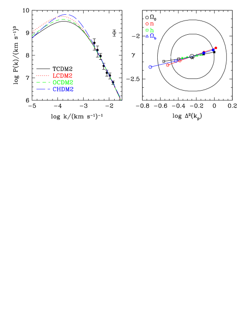
Figure 9: Constraints on the parameters of CDM models obtained by combining the CWPHK $P(k)$ with COBE-DMR normalization. The left panel shows linear mass power spectra of four COBE-normalized CDM models (parameters listed in Table 2), with the inflationary power spectrum index $n$ chosen to give the best match to the measured $P(k)$ (filled circles). The right panel illustrates constraints on the parameters of the LCDM model. The asterisk marks CWPHK’s values of the logarithmic slope $\gamma$ and amplitude $\Delta^{2}\equiv k^{3}P(k)/2\pi^{2}$ of $P(k)$ at wavenumber $k_{p}=0.008({\rm km\;s}^{-1})^{-1}$. Concentric circles show the $1\sigma$ and $2\sigma$ constraints on these parameters. Our fiducial version of the LCDM model predicts the slope and amplitude indicated by the central open circle. Filled (open) points show the effect of increasing (decreasing) one parameter while keeping the others fixed. Each step corresponds to $\Delta\Omega_{0}=0.1$ (circles), $\Delta n=0.05$ (pentagons), $\Delta h=0.05$ (squares), or $\Delta\Omega_{\rm b}=0.01$ (triangles).

Table 2: Parameters of the cosmological models shown in Figure 9. All of these models have $\Omega_{\rm b}h^{2}=0.02$.

Model	$\Omega_{0}$	$\Omega_{\Lambda}$	$\Omega_{\nu}$	$n$	$h$	$\sigma_{8}$
TCDM2	1.0	0.0	0.0	0.84	0.50	0.92
LCDM2	0.4	0.6	0.0	0.88	0.65	0.74
OCDM2	0.55	0.0	0.0	0.88	0.65	0.67
CHDM2	1.0	0.0	0.2	1.10	0.50	0.96

The main assumptions behind this $\Omega_{0}$ constraint are gravitational instability and Gaussian initial conditions. With the more restrictive assumptions of inflation and CDM, we can obtain other constraints on cosmological parameters by combining the Ly$\alpha$ $P(k)$ with COBE-DMR normalization. Figure 9, based on Phillips et al. (1998), shows power spectra of four COBE-normalized CDM models with the inflationary power spectrum index $n$ chosen so that the predicted power spectrum matches the CWPHK result (see model parameters in Table 2). While all of these models can simultaneously match COBE-DMR and the Ly$\alpha$ forest $P(k)$, the high $\sigma_{8}$ values of the $\Omega=1$ models (TCDM2, CHDM2) would imply excessively massive galaxy clusters at $z=0$, in agreement with our earlier, more general argument. The right hand panel of Figure 9 illustrates the constraints from COBE and the Ly$\alpha$ forest $P(k)$ alone in the case of LCDM. With our fiducial parameter choices, this model reproduces the slope and amplitude of the CWPHK $P(k)$ almost perfectly. Changing $\Omega_{0}$, $n$, $h$, or $\Omega_{\rm b}$ in isolation would change the predicted slope and amplitude as indicated. Because the different parameter changes have nearly degenerate effects on the Ly$\alpha$ $P(k)$, our measurement imposes a single constraint on a combination of the parameters:

$$\left(\frac{\Omega_{0}}{0.4}\right)\left(\frac{h}{0.65}\right)^{2.96}\left(\frac{n}{0.88}\right)^{3.92}\;\times$$

$$\left(\frac{\Omega_{\rm b}h^{2}}{0.02}\right)^{-0.445}=1.0\pm 0.5.$$ (4)

As Figure 9 shows, parameter choices that reproduce the measured amplitude of $P(k)$ also reproduce the measured slope. This “coincidence” represents a significant success of the inflation+CDM scenario: the CWPHK measurement confirms its generic prediction of a linear power spectrum that curves steadily towards $k^{n-4}$ on small scales. We plan to apply this technique to a sample of 99 moderate resolution QSO spectra originally obtained by three of us (SB, DK, DT) for the purpose of identifying candidate systems for deuterium absorption studies. The larger sample size will greatly reduce the statistical uncertainties in $P(k)$, leading to tighter constraints on $\Omega_{0}$ and other parameters. A preliminary analysis of this sample yields results within the $1\sigma$ errors of the CWPHK measurement. Figures 4, 7, 8, and 9, and equations (3) and (4), illustrate the power of the Ly$\alpha$ forest as a test of cosmological theories. In contrast to the current situation for galaxies, for the Ly$\alpha$ forest we can predict the form of the “bias relation” (equation 2) based on simple considerations of photoionization and adiabatic cooling. The parameter $A$ that determines the strength of this bias is not well known a priori, but it can be measured for any given model using the mean flux decrement, leaving all other statistical properties of the forest as independent predictions. While these statements are based on the approximate picture of the Ly$\alpha$ forest outlined in §2, hydrodynamic simulations can provide the necessary tests of and corrections to this picture. The most significant corrections — peculiar velocities, thermal broadening, and shock heating — are straightforward to compute with such simulations. The factors that ultimately limit the comparison between models and data are likely to be observational uncertainties in continuum fitting, which make it difficult to measure weak fluctuations on large scales, and theoretical uncertainties in the spatial uniformity of the $\rho-T$ relation. At present it appears that these uncertainties are small compared to the differences between cosmological models. What can we expect to learn from the Ly$\alpha$ forest over the next few years? Most clearly, we should get precise constraints on the amplitude and logarithmic slope of the linear mass power spectrum on scales $\sim 1000{\rm\;km\;s^{-1}}$ at $z\sim 2-3.5$, from application of the CWKH method to larger data sets and from independent checks with HIRES data using statistics like the flux decrement distribution and threshold crossing frequency. Consistency among these statistical properties will test the hypothesis of Gaussian initial conditions. The threshold crossing frequency provides additional constraints on $\Omega_{0}$ and $\Omega_{\Lambda}$ because of their influence on the conversion from comoving $h^{-1}{\rm Mpc}$ to redshift. If continuum fitting can be done with sufficient accuracy, it may be possible to measure curvature of the linear power spectrum or other departures from a power law shape. It should be possible to detect the signature of gravitational growth of fluctuations over the range $z\sim 2-3.5$. Using the rate of growth to constrain $\Omega_{0}$ and $\Omega_{\Lambda}$ probably requires accurate $P(k)$ measurements down to $z\sim 1$, which will be more difficult to achieve because such measurements must be based on HST data and because the physics of the Ly$\alpha$ forest becomes somewhat more complicated at low redshift (Davé et al. 1998). Measurements of the flux autocorrelation or flux power spectrum towards QSO pairs can constrain $\Omega_{\Lambda}$ through its influence on spacetime geometry (CWKH; Hui, Stebbins, & Burles 1998; McDonald & Miralda-Escudé 1998). Finally, all of these results can be combined with complementary constraints from CMB anisotropies, the cluster mass function, Type Ia supernovae, and so forth to test the inflation+CDM scenario of structure formation and to determine the parameters of the universe that we live in.

References

- [1] Bi, H.G., 1993, ApJ, 405, 479
- [2] Bi, H.G., Davidsen, A., 1997, ApJ, 479, 523
- [3] Bi, H., Ge, J., Fang, L.-Z. 1995, ApJ, 452, 90
- [4] Bryan, G. L., Machacek, M., Anninos, P., Norman, M. L., 1998, ApJ, submitted; preprint astro-ph/9805340
- [5] Burles, S., Tytler, D., 1998, ApJ, 499, 699
- [6] Cen, R., Miralda-Escudé, J., Ostriker, J.P., Rauch, M., 1994, ApJ, 437, L9
- [7] Coles, P., 1993, MNRAS, 262, 1065
- [8] Croft, R. A. C., Weinberg, D. H., Hernquist, L., Katz, N., 1997, in Olinto, A., Frieman, J., & Schramm, D. eds., Proceedings of the 18th Texas Symposium on Relativistic Astrophysics. World Scientific, Singapore; astro-ph/9701166
- [9] Croft, R. A. C., Weinberg, D. H., Katz, N., Hernquist, L. 1998a, ApJ, 495, 44 (CWKH)
- [10] Croft, R. A. C., Weinberg, D. H., Pettini, M., Hernquist, L., Katz, N., 1998b, ApJ, submitted; preprint astro-ph/9809401 (CWPHK)
- [11] Davé, R., Hernquist, L., Katz, N., Weinberg, D. H., 1998, ApJ, in press; preprint astro-ph/9807177
- [12] Eke, V. R., Cole, S., Frenk, C. S., 1996, MNRAS, 282, 263
- [13] Fry, J. N., Gaztañaga, E., 1993, ApJ, 413, 447
- [14] Gnedin, N. Y., Hui, L., 1998, MNRAS, 296, 44
- [15] Gunn, J.E., Peterson, B.A., 1965, ApJ, 142, 1633
- [16] Hernquist L., Katz, N., Weinberg, D.H., & Miralda-Escudé, J. 1996, ApJ, 457, L5
- [17] Hui, L., Gnedin, N., 1997, MNRAS, 292, 27
- [18] Hui, L., Gnedin, N., Zhang, Y., 1997, ApJ, 486, 599
- [19] Hui, L., Stebbins, A., Burles, S., 1998, ApJ, submitted; preprint astro-ph/9807190
- [20] Kim, T. S., Hu, E. M., Cowie, L. L., Songaila, A., 1997, AJ, 114, 1
- [21] Kirkman, D., Tytler, D., 1997a, ApJ, 484, 672
- [22] Kirkman, D., Tytler, D., 1997b, ApJ, 489, L123
- [23] McDonald, P., Miralda-Escudé, J., 1998, ApJ, submitted; preprint astro-ph/9807137
- [24] McGill, C., 1990, MNRAS, 242, 544
- [25] Miralda-Escudé J., Cen R., Ostriker, J.P., Rauch, M., 1996, ApJ, 471, 582
- [26] Miralda-Escudé, J., et al. 1997, in Petitjean, P., Charlot, S., eds., Structure and Evolution of the IGM from QSO Absorption Line Systems, 13th IAP Colloquium. Nouvelles Frontières, Paris, p. 155; astro-ph/9710230
- [27] Mücket, J. P., Petitjean, P., Kates, R. E., Riediger, R., 1996, A&A, 308, 17
- [28] Petitjean, P., Mücket, J. P., Kates, R. E., 1995, A&A, 295, L9
- [29] Pettini, M., Smith, L.J., Hunstead, R. W., King, D.L., 1994, ApJ, 426, 79
- [30] Pettini, M., Smith, L.J., King, D.L., Hunstead, R. W., 1997, ApJ, 486, 665
- [31] Phillips, J., Weinberg, D. H., Croft, R. A. C., Hernquist, L., Katz, N., Pettini, M., 1998, in preparation
- [32] Rauch, M., et al., 1997, ApJ, 489, 7
- [33] Scherrer, R. J., Weinberg, D. H., 1998, ApJ, 504, 607
- [34] Theuns, T., Leonard, A., Efstathiou, G., Pearce, F. R., Thomas, P. A. 1998, MNRAS, submitted; preprint astro-ph/9805119
- [35] Wadsley, J. W., Bond, J.R., 1997, in Clarke, D., West, M., eds. Computational Astrophysics, ASP Conference Series 123. ASP, San Francisco; astro-ph/9612148
- [36] Weinberg, D. H., Cole, S., 1992, MNRAS, 259, 652
- [37] Weinberg, D. H., Croft, R. A. C., Hernquist, L., Katz, N., Pettini, M., 1998a, ApJ, submitted; preprint astro-ph/9810011
- [38] Weinberg, D.H., Hernquist, L., Katz, N., Croft, R., Miralda-Escude, J., 1997, in Petitjean, P., Charlot, S., eds., Structure and Evolution of the IGM from QSO Absorption Line Systems, 13th IAP Colloquium. Nouvelles Frontières, Paris, p. 133; astro-ph/9709303
- [39] Weinberg, D. H., Katz, N., Hernquist, L., 1998, in Woodward, C. E., Shull, J. M., Thronson, H., eds., Origins, ASP Conference Series 148. ASP, San Francisco, p. 21; astro-ph/9708213 (WKH)
- [40] White, S. D. M., Efstathiou, G. P., Frenk, C. S., 1993, MNRAS, 262, 1023
- [41] Zhang, Y., Anninos, P., & Norman, M.L. 1995, ApJ, 453, L57