The NTT SUSI DEEP FIELD

Abstract

We present a deep BVrI multicolor catalog of galaxies in a 5.62 sq.arcmin field 80 arcsec south of the high redshift ($z=4.7$) quasar BR 1202-0725, derived from observations with the direct CCD camera SUSI at the ESO NTT. The formal 5$\sigma$ magnitude limits (in $2\times$ FWHM apertures) are 26.9, 26.5, 25.9 and 25.3 in B, V, r and I respectively. Counts, colors for the star and galaxy samples are discussed and a comparison with a deep HST image in the I band is presented. The percentage of merged or blended galaxies in the SUSI data to this magnitude limit is estimated to be not higher than 1%.

At the same galactic latitude of the HDF but pointing toward the galactic center, the star density in this field is found to be $\sim 3$ times higher, with $\sim 20\%$ of the objects with V-I$>$3.0. Reliable colors have been measured for galaxies selected down to $r=26$. The choice of the optical filters has been optimized to define a robust multicolor selection of galaxies at $3.8\leq z\leq 4.4$. Within this interval the surface density of galaxy candidates with $r<26$ in this field is $2.7\pm 0.4$ arcmin^-2 corresponding to a comoving density of Star Formation Rate at $3.8\leq z\leq 4.4$ of $10^{-2.00}\hbox{ - }10^{-1.82}h^{3}\ M_{\odot}\cdot yr^{-1}\cdot Mpc^{-3}$.

1 Introduction

With the implementation of efficient CCD cameras at 4m class-telescopes deep imaging in high galactic latitude fields has become a powerful tool to study galaxy evolution. Since the pioneering work of Tyson (1988), deep ground -based observations have been extended to different color bands (Metcalfe et al., 1995; Smail et al. 1995, Hogg et al. 1997) with image quality of 1 arcsec FWHM or better.

A new benchmark for deep survey work has been set by the Hubble Deep Field observations (Williams et al., 1996). Although the size of the HST primary mirror is 2.5m only and the CCDs in the WFPC2 instrument have relatively poor blue and UV sensitivities, the combination of very long integration time, low sky background and sub-arcsec angular size for most of the faint galaxies in the field, has led to limiting magnitudes which are more than a factor of ten fainter than the deepest ground-based surveys.
The HST observations, beside their intrinsic scientific value, acted as a very efficient catalyst for complementary photometric work in other bands, notably the IR, and for spectroscopic observations of galaxies down to $m_{I}$=25 with the Keck telescope. The project also demonstrated the scientific advantage of dedicating a sizable chunk of observing time to the deep exploration of a single, size-limited field.

The other crucial development in this field has been the identification by the ”Lyman break” technique (Steidel and Hamilton, 1993 ; Steidel, Pettini and Hamilton, 1995) and subsequent spectroscopic follow-up of a large number (a few hundreds known at the beginning of 1998) of $z\sim 3$ galaxies with the Keck telescope (Steidel et al. 1996, Steidel et al. 1998). These results have permitted to address for the first time the issues of star formation rate and clustering at these redshifts, extending the previous spectroscopic survey work (Lilly et al. 1995; Cowie, Hu and Songaila 1995) beyond z= 1.5 .

The Lyman break technique is an example (so far the one with the highest success rate) of the photometric redshift techniques. Since accurate photometry can be obtained for objects at least two magnitudes fainter than the spectroscopic limit, photometric redshifts, that is redshifts which are obtained by comparing broad band observations of galaxies with a library of observed templates or with stellar population synthesis models, are the only practicable way to extend the studies of the population of galaxies at high redshifts ($z\simeq$4 and beyond) to luminosities below $L_{*}$. Photometric redshifts have been derived from ground-based observations to relatively bright magnitude limits and redshifts $z<1$ (Koo 1985, Connolly et al. 1995). The data set of the HDF, which goes much deeper, has revived the interest in this type of work with significant results (Sawicki et al 1997, Connolly et al. 1997 and references therein to earlier work ). Giallongo et al. (1998) have used ground -based observations with the SUSI CCD camera at the ESO New Technology Telescope to measure photometric redshifts for $\sim 200$ galaxies down to a limiting magnitude of $m_{r}=25$.

The observations presented in this paper were obtained for the program ”Faint Galaxies in an ultra-deep multicolour SUSI field”, P.I. S.D’Odorico, approved for ESO Period 58 and executed in service mode also at the ESO NTT in February through April 1997 in photometric nights with seeing better than 1 arcsec. The scientific goals were the study of the photometric redshift distribution of the faint galaxies and of gravitational shearing in the field. The field of view of the SUSI CCD camera is comparable to the HDF, and the goal was to reach limiting magnitudes in the four bands which would enable photometric redshift estimates to $r_{AB}\sim 26.5$ or about 1.5 magnitude fainter than in the previous work by Giallongo et al.(1998). The final coadded calibrated frames have been made available since January 98 at the following address:
http://www.eso.org/research/sci-prog/ndf/.

The chosen field, hereafter referred to as NTT Deep Field or NTTDF, is at 80 arcsec south of the $z=4.7$ QSO BR1202-072 (McMahon et al 1994). It is partially overlapping with the field centered on the QSO and studied in the same 4 optical bands and in K band by Giallongo et al. (1998). The high redshift QSO at the center of the field has several known metal systems in its line of sight spanning from $z=1.75$ to $z=4.7$ (Wampler et al. 1996, Lu et al. 1996) making this field quite interesting for a future comparison between the absorbers and the properties and distribution in redshifts of the field galaxies.

In this paper, we describe the observations, the reduction procedures and the objects catalogue in Section 2, and the galaxy counts and colors in Section 3. The data in the I band are compared with a deep HST observation of the same field and in the same band and more in general with the Hubble Deep Field results in Section 4. The selection of high redshift galaxy candidates is discussed in Section 5 and the conclusions are presented in Section 6.

In a forthcoming paper (Fontana et al. 1998, to be submitted) the data are combined with infrared observations and used to derive the photometric redshifts of the galaxies in the field.

2 The Data Sample

2.1 The Observations

The field centered on $\alpha=12^{h}\ 05^{m}\ 22.4^{s}$, $\delta=-7^{\circ}\ 44^{\prime}\ 12^{\prime\prime}$ was observed in service mode with the SUSI imaging CCD camera at the Nasmyth focus of the ESO New Technology Telescope. The observations have been obtained in four broad band filters, the standard BV passbands of the Johnson-Kron-Cousins system (JKC) and r and i of the Thuan-Gunn system. The CCD was a 1k x 1k thinned, anti-reflection coated device (ESO CCD no. 42). The scale on the detector is 0.13 arcsec/pixel.
The data, including photometric calibrations with standard stars from Landolt (1992), were obtained in the period between February and April 1997. In Table 1, we summarize the observations and list the expected magnitude limits at 5-sigma within apertures of 2$\times$FWHM of the combined frames.

Table 1: Log of photometric observations

Filter	Number of	total	seeing range	Final PSF	Zero-point	$\mu(1\sigma)$	Mag. limit
	frames	exp. time (s)	(arcsec)	(arcsec)	(1)	mag/arcsec2	(5 $\sigma$) (1,2)
B	44	52800	0.74-1.2	0.90	32.60	27.94	26.88
V	26	23400	0.72-1.2	0.83	32.55	27.29	26.50
r	26	23400	0.72-1.2	0.83	31.96	26.58	25.85
I	18	16200	0.60-1.0	0.70	31.81	25.85	25.27

(1) : Magnitude limits and zero-points are provided in natural magnitude systems (see text)
(2) : Magnitude limits are computed inside apertures with diameters of 2$\times$ FWHM without aperture correction (see section 2.3.1).

2.2 Data Reduction

2.2.1 Flat-fielding and coaddition

The single raw frames have been bias-subtracted and flat-fielded. To correct the flat-field pattern, a “super-flat-field” was obtained by using all the dithered images and computing an illumination map with a median filtering at 2.5$\sigma$.
The cosmic rays identification was carried out using the cosmic filtering procedure of MIDAS. A pixel is assumed to be affected by a cosmic ray if its value exceeds 4$\sigma$ of the mean flux computed for the 8 neighboring pixels. These automatic identifications, the positions of known detector defects and of additional events like satellites trails and elongated radiation events detected by visual inspection, were used to build a “mask” frame with “0” values for these pixels and “1” for the others. This defect mask is multiplied by the normalized flat-field to produce the weight map of the individual frames.

To perform the coaddition of all frames, we have applied the same algorithm used for the combination of the HDF frames (Williams et al., 1996), known as “drizzling” (Fruchter & Hook, 1998). The sky-subtracted, dithered images are flux scaled, shifted and rotated with respect to a reference frame corrected for atmospheric extinction. Given the good sampling of the instrument PSF by the CCD pixels, we preserved the input pixel size in the output image. The intensity in one output pixel, $I(x,y)$, is defined as

$$I(x,y)=\frac{\Sigma f_{xy}i(x,y)w_{xy}}{\Sigma f_{xy}w_{xy}}$$ (1)

where $i(x,y)$ is the intensity in the input pixels, $f_{xy}$ is the overlapping area for the input and output pixels and $w_{xy}$ is an input weight taken into account the flux-scaling, r.m.s. and also the weight map of a single frame.

The different number of dithered frames contributing to each pixel of the coadded image produces a non homogeneous noise through the ”drizzled” frame. Each combined frame is accompanied by a combined weight map, produced during the drizzling analysis, which represents the expected inverse variance at each pixel position.

2.2.2 Photometric Calibration

The photometric calibration was obtained from several standard stars from Landolt (1992) observed in the same nights and at similar airmasses. For each standard field, total magnitudes were computed by using a fixed aperture (2.5 arcsec) corrected at 6 arcsec by using the star with the more stable photometric curve of growth.

The $B^{\prime}V^{\prime}R^{\prime}I^{\prime}$ magnitudes are calibrated in the “natural” system defined by our instrumental passbands. The zero points of our instrumental system were adjusted to give the same $BVRI$ magnitudes as in the standard JKC system for stellar objects with $B-V=V-R=R-I=0$. The colour transformations used for stellar objects are : $B^{\prime}=B-0.14\times(B-V)$, $V^{\prime}=V-0.08\times(B-V)$, $R^{\prime}=R-0.33\times(V-R)$ and $I^{\prime}=I+0.01\times(V-I)$.

In order to derive the zero-point fluxes, for each scientific frame the closest (in time) standard field has been analyzed and reduced to the same airmass. The flux-scale factor corresponding to this scientific frame is used to provide the final-zero-point. The zero-point estimations for all standard fields are consistent within 0.03 mag and are given in Table 1. The following extinction coefficients were adopted: $k_{B}=0.22,k_{V}=0.11,k_{r}=0.05,k_{I}=0.02$.
Finally, the transformations to the AB systems are given by these relations : $I_{AB}=I^{\prime}+0.47$, $r_{AB}=R^{\prime}+0.21$, $V_{AB}=V^{\prime}$, $B_{AB}=B^{\prime}-0.16$.

2.3 Data extraction

2.3.1 Object Detection and Magnitudes

The analysis of “drizzled” images were performed with the SExtractor image analysis package (Bertin & Arnouts, 1996).

The detection and deblending of the objects has been carried out using as a reference the weighted sum of the $B\leavevmode\nobreak\ V\leavevmode\nobreak\ r\leavevmode\nobreak\ I$ bands (in the following combined image). The weight assigned to each band is proportional to the signal-to-noise of the sky in the individual weight-map.

The use of the combined image insures an optimal detection of normal or high redshift objects but also of any peculiar objects with strong emission lines in the bluest bands. The object detection is performed by convolving the combined image with the PSF and thresholding at 1.1$\sigma$ of the resulting background RMS. The catalogue of the detections is then applied to each of the four individual frames.

To estimate the total magnitudes, we used the procedure described by Djorgovski et al. (1995). For the brighter objects, where the isophotal area is larger than 2.2 arcsec aperture (17 pixels) (corresponding roughly to $B\leq$25, $V\leq$24.5, $r\leq 24$ and $I\leq 23.25$), we use an isophotal magnitude above a surface brightness threshold of 1.$\sigma$ of the sky noise. For objects with smaller isophotal area, we used the 2.2 arcsec aperture magnitude (corresponding to 2-3 FWHM), corrected to a 5 arcsec aperture by assuming that the wings follow a stellar profile. The corrections are independent of the magnitude and correspond to -0.15, -0.14, -0.13, -0.09 mag for B, V, r, I respectively. The validity of this assumption has already been tested in previous similar deep images (Smail et al. 1995). Finally, the magnitudes were corrected for galactic absorption with $E(B-V)=0.03$ by using $A_{B}/A_{V}=1.33$, $A_{r}/A_{V}=0.83$ and $A_{I}/A_{V}=0.59$ where $A_{V}=3.1\times E(B-V)$.

In this procedure several objects detected in the combined image are either too noisy to obtain a reliable magnitude or undetected in the individual drizzled frames. Objects with a computed magnitude within a 2.2 arcsec aperture fainter than the expected magnitude limit at 2$\sigma$ (i.e. $B\sim 27.57$, $V\sim 26.95$, $r\sim 26.29$, $I\sim 25.57$) have been assigned an upper-limit magnitude.

2.3.2 Star-galaxy Separation

For the star-galaxy separation, we used the classifier provided by SExtractor applied to the I band, to which corresponds the best PSF. This classifier gives output values in the range 0-1 (0 for galaxies and 1 for stars). For I$\leq$24 an object is defined stellar if the classifier has a value larger than 0.9. For fainter magnitudes no star/galaxy separation is carried out. The combination of bright cut-off in magnitude and high value for stellar index insures that the stellar sample is not contaminated by unresolved galaxies. In section 4.3, the efficiency of our criterion is compared with HST data.

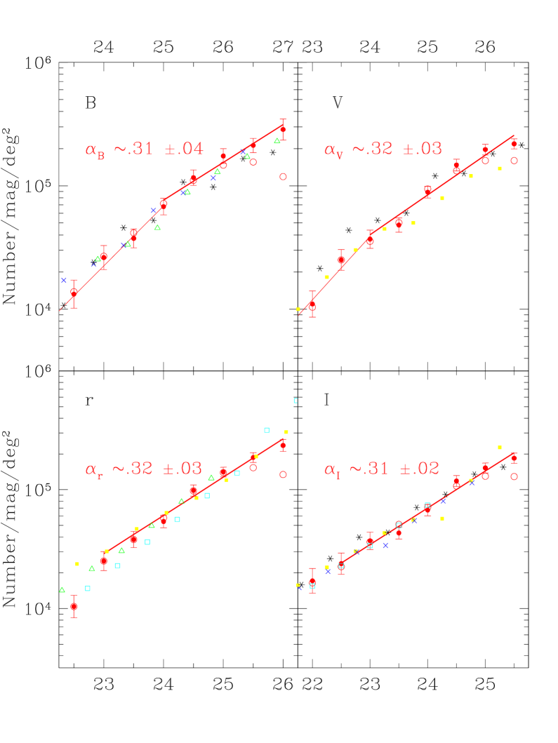
Figure 1: Differential galaxy number counts for the B, V, r and I bands. Open circles show the raw counts and filled circles show the corrected counts for incompleteness. The error bars include the correction factor, the density fluctuation and poisson errors. The large solid lines give the best fits for the slope. The previous works are drawn with different symbols. They include the data from Tyson (1988, open squares), Lilly et al. (1991, crosses), Metcalfe et al. (1995, triangles), Smail et al. (1995, filled squares), Williams et al. (1996, stars). Our $r$ filter is significantly different to the R Cousins, thus we have applied to the previous works a shift of 0.2 ($r=R-0.33(V-R)$, by assuming $<V-R>\sim 0.6$).

Table 2: Number counts and errors

magnitude	Number counts $(N_{cor})$	$\sigma_{tot}$	Completeness	$\sigma_{pois}/N_{cor}$	$\sigma_{clust}/N_{cor}$	$\sigma_{comp}/N_{cor}$
	$(10^{4}\ deg^{-2}.mag^{-1})$	$(10^{4})$	factor	(%)	(%)	(%)
B
23.5	1.32	0.35	0.96	0.9	26.2	1.2
24.	2.62	0.59	0.98	0.6	22.5	0.9
24.5	3.75	0.66	0.91	0.5	17.5	0.7
25	6.78	1.05	0.95	0.4	15.4	0.5
25.5	11.65	1.69	1.05	0.3	14.5	0.4
26	17.42	2.39	1.18	0.3	13.7	0.4
26.5	21.25	2.82	1.36	0.3	13.3	0.4
27	28.58	5.64	2.41	0.3	19.7	0.5
V
23.	1.10	0.27	1.06	1.0	24.4	1.4
23.5	2.51	0.49	1.00	0.6	19.4	0.9
24.	3.69	0.63	1.04	0.5	17.0	0.8
24.5	4.81	0.64	0.96	0.4	13.2	0.6
25	8.89	0.97	0.95	0.3	10.9	0.5
25.5	14.75	1.60	1.11	0.3	10.9	0.4
26	19.67	1.98	1.23	0.2	10.1	0.3
26.5	21.88	2.06	1.37	0.2	9.4	0.3
r
22.5	1.04	0.23	1.00	1.0	21.8	1.3
23.	2.51	0.46	1.00	0.6	18.3	0.9
23.5	3.81	0.59	1.00	0.5	15.4	0.7
24.	5.40	0.65	0.93	0.4	12.1	0.6
24.5	9.85	1.08	1.01	0.3	10.9	0.4
25	14.09	1.31	1.01	0.3	9.3	0.4
25.5	18.64	1.76	1.22	0.3	9.4	0.4
26	23.55	2.69	1.75	0.3	11.4	0.4
I
22.	1.71	0.41	1.04	0.8	24.0	1.1
22.5	2.39	0.49	1.06	0.7	20.6	0.9
23.	3.71	0.62	1.02	0.5	16.7	0.8
23.5	4.32	0.50	0.90	0.4	11.6	0.6
24.	6.73	0.74	0.95	0.4	11.0	0.5
24.5	11.82	1.27	1.10	0.3	10.7	0.4
25	15.24	1.47	1.17	0.3	9.6	0.4
25.5	18.41	1.81	1.43	0.3	9.8	0.4

2.3.3 Astrometry

The astrometry uses a tangent-projection to transpose the pixel coordinates to RA and Dec (equinox 2000). The transformation has been calibrated with 15 objects, well distributed over the whole SUSI field, selected in the APM catalogue at the following URL:
http://www.ast.cam.ac.uk/$\sim$apmcat.

A first solution of the astrometry was computed with a polynomial fit which provides a residual error lower than 0.1 arcsec. Then the astrometric parameters have been derived for a tangent-projection solution and are again consistent with APM at better than 0.1 arcsec. To check the reliability of our astrometry, we have compared with a WFPC2 image close to the field. In the overlapping region, 108 common objects are detected. A systematic shift of 0.69 $\pm$ 0.10 arcsec in alpha and -0.70 $\pm$ 0.10 in delta is observed. The relative astrometric error is close to 0.1 arcsec and the systematic uncertainty is compatible with the value given by the APM catalogue ($\sim$ 0.5 arcsec).

2.4 The Catalogue

All the data used in this paper are available in a catalogue present at the following URL address:
http://eso.hq.org/research/sci-prog/ndf.
The catalogue is accompanied by a description file. The identification number, position (pixels and astrometric coordinates), total magnitudes and errors in each band are given. Star/galaxy classification and morphological parameters have been obtained from the I band. To estimate colors the I frame has been smoothed to match the seeing of the other bands (see section 3.2).

Figure 2: Color-magnitude diagram for $(B-V)$ versus $r$ and $(B-r)$ versus $r$ in our natural systems. The colors are computed in fixed aperture of 15 pixels. Open circles represent the colours at 2$\sigma$, open triangles the colours at 1$\sigma$ and stars show the stellar objects. The large filled points are the medians colors. The horizontal bars show the extent of magnitude bin. For magnitudes fainter than 23, the medians are computed for 60 objects per bin. The vertical error-bars give the 1$\sigma$ error calculated using boot-strap resampling of data. Comparison with Arnouts et al. (1997,short dashed line) and Metcalfe et al. (1995, long dashed line) are shown by applying the color correction given in sect. 2.2.2.

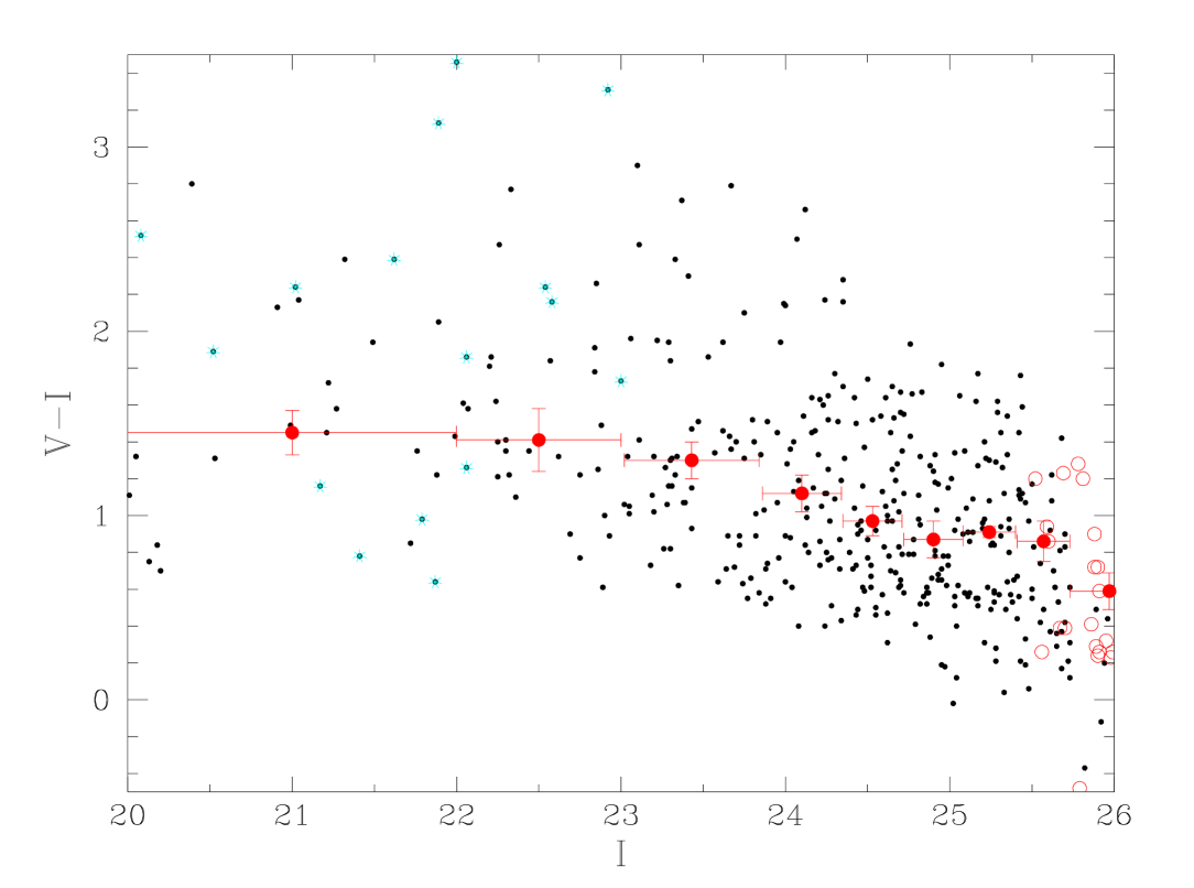
Figure 3: Same as figure 2 for $(V-r)$ versus $r$ and $(V-I)$ versus $I$. Comparison with Arnouts et al. (1997, dashed line) and Smail et al. (1995, solid line) are shown by applying the color correction given in sect. 2.2.2.

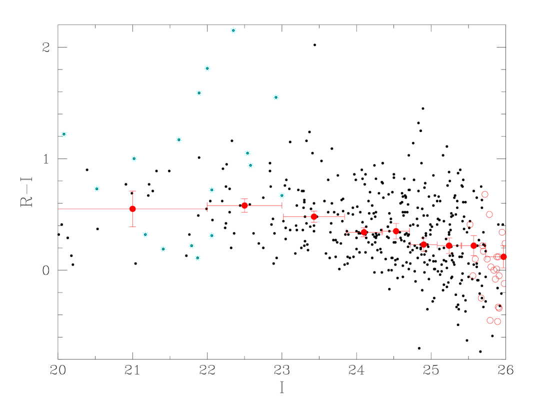
Figure 4: Same as figure 2 for $(B-I)$ versus $I$, and $(r-I)$ versus $I$. Comparisons are shown for the data from Tyson (1988, solid line) and Lilly et al. (1991, dashed line) by applying the color correction given in sect. 2.2.2.

3 Counts and colors

3.1 Differential Galaxy Counts

Before discussing the galaxy counts, we have to apply a correction for completeness at faint magnitudes. A standard way to estimate the fraction of lost sources, crowding, spurious objects, magnitude errors, etc …, is to generate simulations by assuming a typical profile for all kinds of galaxies and different cosmological models (Metcalfe et al, 1995). In the present case, we have to take into account that the detection of sources has been done by using the combined image of the four bands and that the noise in our drizzled frame is correlated due to the drizzling algorithm. To provide an estimation of the correction as close as possible to the characteristic of our raw data, we have adopted the following empirical approach:

1. we extract objects in the magnitude ranges 23$\leq B,V\leq$ 25.5 and 23$\leq r,I\leq$25.0 (by using the “check-images” tool of SExtractor software). At these magnitudes, the signal-to-noise is greater than 8.

2. the object’s fluxes are dimmed by factors 4, 6.5 and 10 and added randomly to the original frames (combined image and $B\leavevmode\nobreak\ V\leavevmode\nobreak\ r\leavevmode\nobreak\ I$ images). The noise in the resulting combined and $B\leavevmode\nobreak\ V\leavevmode\nobreak\ r\leavevmode\nobreak\ I$ images is identical to the original data.

3. The algorithm of detection is applied to the combined image and the measure of the magnitudes is carried out on the $B\leavevmode\nobreak\ V\leavevmode\nobreak\ r\leavevmode\nobreak\ I$ frames. The correction factor for each magnitude bin is derived from the fraction of the “simulated” sources that are detected.

The magnitude range of the original sources used in this simulation has been chosen in a way that a sufficient number of objects between $24.5-27.5$ is generated, while avoiding a too large crowding at intermediate magnitudes. Besides, since the original galaxies have a mean expected redshift of 0.6-1.0 and we do not expect drastic differences of colors with respect to the fainter galaxy population (except for the ellipticals in the B band), this allows us to ignore any additional k-correction term. Note that this analysis doesn’t include the Eddington bias and can overestimate the correction factor. The completeness factor ($f=\frac{N_{simul}}{N_{detect}}$) is reported in table  2.

In Fig. 1, we plot the raw and corrected differential galaxy counts as a function of the magnitude ($N_{cor}=N_{raw}.f$) and we report the corrected number counts in table  2. The error bars include the quadratic sum of the Poisson noise ($\sigma_{pois}$), the uncertainty in the completeness factor ($\sigma_{comp}$) and the clustering fluctuation due to the small size of the field as follows :

$$\sigma^{2}_{clust}=<N_{cor}>^{2}\frac{A_{\omega}}{\Omega^{2}}\int\theta_{12}^{-0.8}d\Omega_{1}d\Omega_{2}$$ (2)

$$\sigma^{2}_{clust}=<N_{cor}>^{2}\ A_{\omega}\ IC$$ (3)

where IC is the integral constraint computed by a Monte-Carlo method for the appropriated size of the NTTDF field ($IC=33.58$). The relationship between the amplitude $A_{\omega}$ and the magnitude is assumed to evolve as $A_{\omega}(at\ 1^{\circ})=-0.3*mag+C_{tt}$, where $C_{tt}=4.4,4.1,3.9,3.8$ for the B, V, r and I bands respectively. The individual and total errors are reported in table  2.

The slopes are estimated by linear regression. For the B and V bands, the counts show a significant flattening at magnitudes fainter than B$\sim$ 25 and V$\sim 24$ with slope values of $\alpha_{B}=0.31\pm 0.04$ and $\alpha_{V}=0.32\pm 0.03$. The evidence of breaks in the B and V bands have been already produced by previous works (Metcalfe et al. (1995), Smail et al. (1995)). The low density of bright galaxies in the NTTDF produces an artificially steep slope at bright magnitudes, making more apparent the breaks in the counts at 25 and 24 in B and V.

The slopes at faint magnitudes in the B and V bands are similar to those observed in the whole range in r and I bands :
$\alpha_{r}=0.32\pm 0.03$ with $23\leq r\leq 26$ and $\alpha_{I}=0.31\pm 0.02$ with $22.5\leq I\leq 25.5$.

In Fig. 1, our results are compared with the previous works of Tyson (1988), Lilly et al. (1991), Steidel et al. (1993), Metcalfe et al. (1995), Smail et al. (1995) and Williams et al. (1996). At bright magnitudes, the discrepancy is large ($\pm 0.1$ in the slope) due to the bias mentioned above. At faint magnitudes the slopes are consistent among the different works.

3.2 Colours of the Galaxies in the Sample

To measure colours, we have smoothed the I frame to the same effective seeing of the worst frame (B frame) and carried out photometry in 2 arcsec diameter apertures with the same center as defined in the summed frame. The colors versus magnitude plots are shown in Fig. 2, Fig. 3,Fig. 4. The 2$\sigma$ and 1$\sigma$ color limits within the 2 arcsec apertures are represented by open circles and triangles respectively. The median include the colour limits at 1 and 2 $\sigma$ and has been computed in bins with 60 objects except for bright magnitudes where bins extending from 20 to 22 and from 22 to 23 have been imposed. The error bars on the median colours have been computed by using a boot-strap resampling method. A comparison with previous works is shown with solid and dashed lines. This comparison has to be taken with caution because the colors are estimated with constant number of objects in each bin and not with a fixed bin. All the color distributions show up to r$\simeq$24-24.5 a blueing trend at bright magnitudes. At deeper magnitudes, the median $B-V$, $B-r$ and $V-r$ versus $r$ (Fig. 2,  3) show stable values. The $B-I$, $V-I$ and $r-I$ versus $I$ (Fig. 3 and Fig. 4) show again a blueing trend but no color stabilization is observed at the fainter magnitudes. This flattening in the various colors is in good agreement with the observed convergence of the slopes ($\sim$ 0.32) in the differential counts for all the four filters.

3.3 Magnitudes and Colours of the Stellar Objects

A by-product of this catalogue is a sample of stellar objects. As in the case of the HDF, the study of the stellar population present in the NTTDF can give useful insight in the galactic structure and/or give constraints on the baryonic dark matter. With the NTTDF it is possible to perform a direct comparison of its stellar content with the one of the HDF. The two fields have essentially the same galactic latitude (for NTTDF $b=53.4$ and for HDF $b=54.8$), but different galactic longitude, with the NTTDF pointing toward the galactic center ($l=283.6$), while the HDF is pointing toward the galactic anti-center ($l=125.6$). Moreover, they cover essentially the same area in the sky ($\simeq 0.0016$ square degrees), allowing us to make a direct comparison of the two stellar samples.

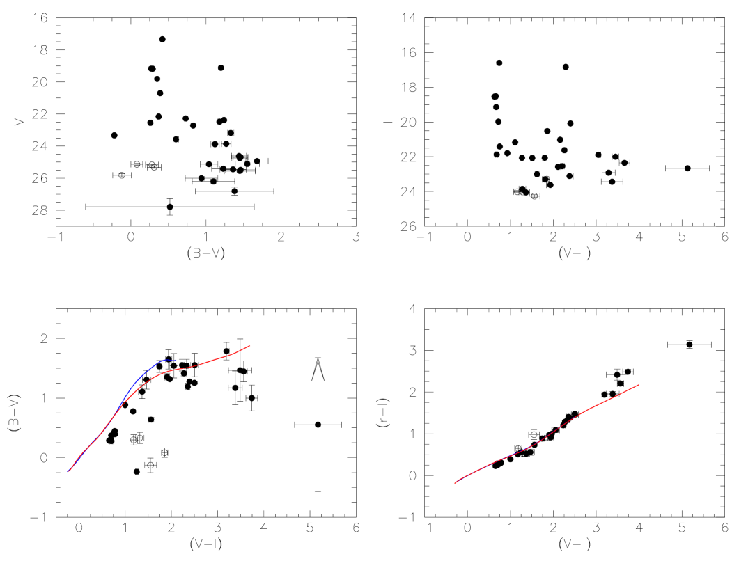
Figure 5: In these plots we present the color-magnitude and color-color diagrams of the objects classified as stellar in the NTTDF. Upper Left. V vs.(B-V) color-magnitude diagram. Upper Right. I vs.(V-I) color-magnitude diagram. Lower Left. (B-V) vs. (V-I) color-color diagram. Lower Right. (r-I) vs. (V-I) color-color diagram. Continuous lines are the colors expected for giants/dwarfs stars (from Caldwell et al. 1993).

In the upper panels of Fig.5 we show the V vs.(B-V) and I vs.(V-I) color-magnitude diagrams of the objects classified as stellar (star/galaxy class$\geq 0.9$) in our final catalog. The objects selected have colors in good agreement with the color expected for stellar objects. In the lower panels of Fig. 5 we have put the (B-V) vs.(V-I) and the (r-I) vs.(V-I) color-color diagrams. It can be clearly seen that, especially in the (r-I) vs.(V-I) (where the observational errors are lower), the objects follow very closely the colors expected for giants/dwarfs stars (the continuous lines are taken from Caldwell et al. 1993), assuring us that the classification parameter gave reliable results. In all the plots we have also included 4 objects with star/galaxy class$\geq 0.8$ and $<0.9$ (shown as open dots). These blue objects have been included since they resemble the population of blue objects found by Mendez et al. (1996) in their analysis of the stellar content of the HDF: they could be interpreted as partially unresolved blue galaxies. In this sample the object in the (B-V) vs.V diagram at V$\simeq 23.2$ is the brightest and bluest member of this sample.

Of some interest for a follow up spectroscopic observation is the object #606 of the catalogue, having a (V-I)$\simeq 5.2$. The colors of this object, including an infrared (I-K)=3.2 (Fontana et al. 1998, to be submitted), are consistent with those expected for bright low mass stars (Delfosse et al 1998). This object has also colors very similar to KELU-1, a field brown dwarf with a mass below $0.075M/M_{\odot}$, and a distance from the Sun of $\sim 12$pc (Ruiz, Legget, & Allard 1997). Other likely faint brown dwarfs are the 5 objects with $3.2<(V-I)<4.0$; their catalogue number is: #93, 112, 249, 579, 600.

In our (V-I) vs.I diagram we don’t have stars below I$\simeq 24$, even if our detection limit is I$\sim 25.6$. This difference could be explained by the fact that are needed at least 5 times more photons to classify objects rather than just detect them (Flynn et al. 1996). In the magnitude range $20<$I$<24$ we found 26 objects, with 6 objects at (V-I)$>3$ ($\sim 20\%$ of this sample). The number of objects are approximately 3 times the stars detected in the same magnitude range in the HDF (see Flynn et al. 1996, Mendez et al. 1996, Reid et al. 1996 for different results on the HDF). This difference in number may be explained by the fact that the NTTDF is pointing in the direction of the galactic center. It is compatible with the prediction obtained with the galactic model by Robin and Creze (1986), as available at www.ons-besancon.fr/www/modele_ang.html.

Finally, The object #570, classified as stellar-like on the basis of the SExtractor algorithm, is listed in the catalog by Giallongo et al 1998 (where it is #12) with colors typical of an high redshift candidate. Cowie and Hu (1998, private communication) obtained a spectrum at Keck. Although the S/N is low, an M star interpretation of the spectral features appears more likely. The colors of the object (including the $I-K\simeq$1.5 of Fontana et al. 1998) would be marginally consistent with a slightly earlier (K5-K7) classification. In Sect. 5 (see in particular Fig. 9) it will be shown that few red stars display colors similar to high-z galaxies.

4 Comparison with the Hubble Space Telescope

4.1 HST Observations of the same field

We compared the NTTDF I-band image photometry with the photometry of WFPC2 archival images of the same field. The WFPC2 data consisted in a set of 8 F814W images totaling 9200 sec of exposure, with the QSO BR1202-0725 centered on CCD #3. Of the four WFPC2 CCD we used only CCD #2 which was almost completely overlapping ($\leavevmode\nobreak\ 90\%$ of the frame) on the North-East corner of the NTTDF I-band image. We carried out a completely independent analysis of the WFPC2 data from the NTTDF data, since we wanted to investigate the consistency of the two data sets and in particular the impact of the lower angular resolution of the ground-based observations on the morphological and the star/galaxy classification algorithm of SExtractor.

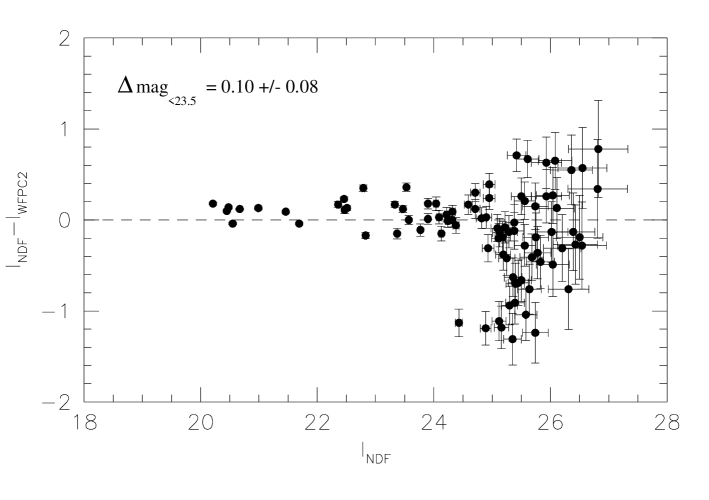
Figure 6: Magnitude comparison of the NTTDF and WFPC2 photometries.

The photometry of the objects in the WFPC2 image was performed on the coadded and cosmic ray cleaned image. We used a detection threshold of $\sim 1.0\sigma$ of the sky noise and a FWHM of 1.5 pixels, finding 132 objects. The estimated magnitude limits at $5\sigma$ in an aperture of $2\times$FWHM ($\simeq 0.\!^{\prime\prime}3$) is I${}_{AB}=24.21$. The data have been calibrated in the STMAG system of the WFPC2, correcting the zero point to the AB system with
ABMAG=STMAG$-0.819$ (Williams et al 1996).

Figure 7: Comparison of the star/galaxy classification in the NTTDF and WFPC2 photometries. Open dots are objects classified as stars in the WFPC2 image, while filled dots are objects classified as galaxies in WFPC2.

Figure 8: Comparison of the ellipticity estimation in the NTTDF and WFPC2 photometries.

4.2 Matching WFPC2 and NTTDF catalogue of objects

We used the astrometric solution for the WFPC2 data (obtained with the metric command of IRAF) to match the objects in the NTTDF. After eliminating a residual shift of $0.\!^{\prime\prime}69\pm 0.10$ in RA, and $-0.\!^{\prime\prime}70\pm 0.10$ in Dec (these values are within the expected values for the HST pointing precision), we found 108 common objects in the two lists. The matching has been done finding the nearest object in the WFPC2 catalog for each object in the NTTDF catalog, with a maximum tolerance of 1 arcsec.

In the common area only 10 WFPC2 objects were not found in the NTTDF image, and 40 NTTDF objects were not recovered in the WFPC2 image. We verified the nature of these non-matched objects looking the morphology of each of them in both images. In the case of the 10 non-matched objects detected in the WFPC2 image we found that one of them was a blend of a relatively bright star and a galaxy in the NTTDF frame, while 4 other objects were clearly “blobs” (star formation regions?) associated to some extended objects. The remaining 5 objects were just at the detection limit in the WFPC2 image and barely visible objects in the NTTDF image, just below the detection threshold. Using this number, we conclude that a reasonable estimate of the frequency of blended objects in the NTTDF field should be $\simeq 1\%$.

The large number of objects present in the NTTDF catalogue and not found in the WFPC2 image (40) is due to the fact that the NTTDF catalog was obtained using the summed image of the four different bands. This means that many of the objects were not present also in the I-band image of the NTTDF. In fact, a direct inspection of the two images at the location of the 40 non-matched objects revealed that all the objects missed in the WFPC2 image were at the detection limit in the NTTDF, and that no bright object was missed: 16 out of 40 objects were classified as having upper limit magnitudes in the NTTDF catalog, and the remaining 24 had a magnitude below $\simeq 25.0$. All these objects are barely visible in the WFPC2 image.

4.3 Magnitude and morphology comparison

Fig. 6 shows the comparison of the photometry of the NTTDF I-band image with the WFPC2 in the almost equivalent F814W band. We selected only the 86 object having the SExtractor flag $\leq 3$ (only isolated objects or with marginal blending) in both the NTTDF and WFPC2, and excluding all the objects with upper limits. The isophotal magnitude difference between NTTDF and WFPC2, computed for objects brighter than 23.5, gives a mean value of $0.10\pm 0.08$ mag. This difference is compatible with the uncertainties in the absolute calibration of the two photometric systems.

Despite the broadening of the stellar profiles due to the effect of the seeing, the comparison of the the star/galaxy classification of the NTTDF objects and the one of the WFPC2 shows a remarkable agreement. In Fig. 7 we show the two classifications using filled circles for objects with the classifier $<0.90$ (galaxies) in the WFPC2 frame and with open circles for objects with $\geq 0.90$ (stars) in WFPC2. The figure shows that of the 9 objects classified as stars down to the 25 mag in WFPC2, only one is misclassified as a galaxy in the NTTDF. This means that the residual contamination of stars down to the magnitude 25 should be $\simeq 1.5\%$ (1 star out of 78 galaxies).

Figure 9: Color criteria to select star forming galaxies at redshift 3.8 $\leq z\leq$ 4.4. Triangles show objects with $B-I$ upper limits distant less than 1$\sigma$ from the color selection criterion, circles show objects with upper limits distant between 1 and 2$\sigma$ from the selection criterion. Both are considered as upper-limits (defined with arrows). The galaxy with B and V upper-limit and filled triangle (# 596 in the catalogue) is spectroscopically confirmed at $z\simeq 4.2$. Stars (with stellarity index $\geq$0.9) are shown with star symbols. For clarity, error-bars are put only for galaxies matching the color criteria.

The comparison of morphological shape parameters (minor and major axis, inclination ($\theta$), ellipticity) of the NTTDF with the one of the WFPC2 revealed that ground-based observations recover the shape parameters within an accuracy of 30% only. We give an example in Fig. 8 where we compare the ellipticity parameter for galaxies brighter than 25 mag and with a total area greater than 25 WFPC2 pixels (38 objects). We cannot find object with ellipticity above $\sim 0.4$ in the NTTDF while in the WFPC2 we can easily reach a value of $\sim 0.75$: this “roundization” effect is first due to the atmospheric seeing and second to the coadding of dithered frames of different image quality.

4.4 The Hubble Deep Field

The Hubble Deep Field project (Williams et al 1996) has set a new benchmark for multicolor deep survey. The total integration time dedicated to the HDF was significantly longer than for the NTTDF (506950 seconds versus 115800). A measure of the relative speeds in collecting photons can be made for the B and I bands, which are the only ones to be relatively similar. The HST F450W band is wider and shifted by about 30 nm to the visual than its SUSI counterpart, while the F814W is close to the corresponding SUSI I band. The integration times on the HDF are a factor of 2.3 and 7.6 longer in the two bands respectively. The factors which enter in the determination of the limiting magnitudes are, beside the exposure times, the ratio of collecting areas between the two telescopes and the efficiency of the light path, including mirrors, instrument optics, filter pass bands and detector. By using the values given by Williams et al. 1996 for the HST (their figure 2) and the computed values for SUSI, we derive a relative efficiency SUSI/ HST, including the ratio of the collecting areas, of 5 in both B and I respectively. The additional two important factors in determining the limiting magnitude are the sky surface brightness and the size of the images. For stellar objects, when the magnitude is computed within 2 FWHMs of the Gaussian fit, the HST takes maximum advantage of the superior image quality because the background is both of lower surface brightness and computed over a smaller area. The limiting magnitudes of the HDF are a factor of 6 and 11 deeper than those of the NTTDF. The gain is reduced to a factor of 2 and 7 for diffuse objects with 2 x FWHM $\geq$ 1 arcsec.

5 The multicolor selection for high redshift galaxies

Steidel & Hamilton (1993) used a combination of three filters U, G and ${\cal R}$ to select star forming galaxies at 2.8$\leq z\leq$ 3.4. At these redshifts, due to the shift of the Lyman continuum break in the UV band, the U flux is attenuated and the $U-G$ color is strongly reddened while the $G-{\cal R}$ color still reflects a flat spectrum.
To select galaxies at higher redshifts, a different set of filters is required. At $z\sim$4, the combination of Lyman $\alpha$ clouds absorption and the Lyman continuum reduces significantly the observed flux also in the B filter. Giallongo et al. (1998) have shown that an optimized set of filters can be found to detect star forming galaxies at $z\simeq 4$ and to reduce the confusion with low redshift galaxies of similar colors. This set is based on the B,V,r and I bands, and corresponds to the one adopted in the present work. An optimized detection of star forming galaxies in the redshift range 3.8$\leq z\leq$4.4 can be obtained by using the following criteria : $(B-I)_{AB}\geq$2, $(V-I)_{AB}\geq$0.5 and $(r-I)_{AB}\leq$0.1. In Figure 9, we have applied the criteria to our catalogue. Two approaches have been followed to select galaxy candidates up to $r\leq 26$.

• A: Galaxies with measured colors (or upper limits) located inside the area defined by the above criteria (8 galaxies).

• B: The above sample and galaxies with $(B-I)_{AB}$ upper limits falling less than $1\sigma$ outside the selection criterion (15 galaxies).

The photometric redshifts for the galaxies of this field will be estimated in a forthcoming paper (Fontana et al., 1998) by comparing the colors (including J and K) with a library of synthetic galaxy spectra as described by Giallongo et al. (1998). Due to their faint magnitudes, the spectroscopic confirmation of our candidates requires an 8-m class telescope. Only one of the galaxies (object # 596 in our catalog) is included in the spectroscopic sample by Hu et al. (1998) and Hu (1998,private communication) and has a spectroscopic redshift of $z\simeq 4.19$. This galaxy has upper limits in the B and V bands and a magnitude $r\simeq 25.9$.
The number of galaxy candidates in different magnitude intervals are given in Table 3 and Table 4 for both classes $A$ and $B$ described above. The surface density at $r\leq$25, is in the range 0.7-0.9 arcmin^-2 (case $A$ and $B$ respectively). At $r\leq$26, the density increases to 1.4-2.7 arcmin^-2.

Table 3: Number distribution of galaxies in redshift range $3.8\leq z\leq 4.4$ located inside the color selection criteria (case A with 8 objects).

$r$	Num.	up.-lim.	up.-lim.	cum. dens.
		B	B & V	(arcmin2)
24$\leq r\leq$ 24.5	1	0	0	0.2
24.5$\leq r\leq$ 25	3	2	0	0.7
25$\leq r\leq$ 25.5	2	2	0	1.1
25.5$\leq r\leq$ 26	2	2	1	1.4

Table 4: Same as Table 3 for case B (with 15 galaxies).

$r$	Num.	up.-lim.	up.-lim.	cum. dens.
		B	B & V	(arcmin2)
24$\leq r\leq$ 24.5	1	0	0	0.2
24.5$\leq r\leq$ 25	4	3	0	0.9
25$\leq r\leq$ 25.5	4	4	0	1.6
25.5$\leq r\leq$ 26	6	6	2	2.7

Assuming a uniform redshift distribution of the sample in the range 3.8$\leq z\leq$4.4, the comoving galaxy number density at $<z>\simeq 4.1$ for $r\leq 25$ is estimated to be $6.5-8.1\leavevmode\nobreak\ 10^{-4}h^{3}Mpc^{-3}$ (q₀=0.5) and $1.3-2.4\leavevmode\nobreak\ 10^{-3}h^{3}Mpc^{-3}$ (q₀=0.5) for r$\leq 26$.

The star formation rate history at $z\simeq$ 4.1 can be derived from the luminosity in the I band corresponding to the restframe wavelength 1500 Å. We adopt the conversion factor (from the UV luminosity at 1500 Å to the SFR) of Madau et al. (1996). For a Salpeter IMF (0.1$\leq M\leq 125M_{\odot}$) with constant SFR, solar metallicity and age range of 0.1-1 Gyr, a galaxy with $SFR=1M_{\odot}\cdot yr^{-1}$ produces $L_{1500}=10^{40.15\pm 0.02}\ erg.s^{-1}\cdot\AA^{-1}$.
The brightest galaxy in our sample has a magnitude of $I_{AB}=24.5$ corresponding to a $SFR=15.0\pm 1.5\ (55\pm 8)h^{-2}\ M_{\odot}\cdot yr^{-1}$ for $q_{0}=0.5$ ($q_{0}=0.05$), and the faintest one has a magnitude of $I_{AB}=26.6$ corresponding to a $SFR=2.2\pm 0.3\ (8\pm 2)\ h^{-2}\ M_{\odot}\cdot yr^{-1}$ for $q_{0}=0.5$ ($q_{0}=0.05$) (the uncertainties are linked to the redshift range $3.8\leq z\leq 4.4$).
Assuming that the redshift range is uniformly probed, the star formation rate per unit comoving volume at $z\simeq 4.1$ derived from objects with $r\leq 25$ varies (for cases $A$ and $B$, respectively) between $10^{-2.21}-10^{-2.14}\ (10^{-2.49}-10^{-2.42})\leavevmode\nobreak\ h^{3}\cdot M_{\odot}\cdot yr^{-1}\cdot Mpc^{-3}$ with $q_{0}=0.5$ ($q_{0}=0.05$). For $r\leq 26$, the estimates increase to $10^{-2.00}-10^{-1.82}\leavevmode\nobreak\ (10^{-2.28}-10^{-2.10})\leavevmode\nobreak\ h^{3}\cdot M_{\odot}\cdot yr^{-1}\cdot Mpc^{-3}$ with $q_{0}=0.5$ ($q_{0}=0.05$).
This latter estimate is close to the value of $10^{-2.06\pm 0.2}M_{\odot}\cdot yr^{-1}$$\cdot Mpc^{-3}$ computed by Madau (1997) for the HDF in the same redshift interval down to $V\leq 28$

6 Discussion and Conclusions

We have presented the first results of a deep multi-colour (B, V, r, I) field observed at ESO with the NTT telescope. A full description of the data reduction and analysis has been given. The final images and catalogue are available on the WEB site of ESO.

A comparative study with a WFPC2-HST image of the same field allows us to estimate the image quality of the NTTDF. Despite the broadening of the stellar profiles due to the effect of the seeing, the comparison of the the star/galaxy classification of the NTTDF objects and the one of the WFPC2 shows good agreement. Reliable star/galaxy separation is obtained down to I$\simeq$24 where the star contamination of the galaxy sample is $\simeq$1.5%. The comparison of the stellar content of the NTTDF with the one of the HDF indicates that the star density in the NTTDF is $\sim 3$ times higher, and of the 26 stars in the magnitude range $20<I<24$, 6 are low mass stars or possible brown dwarfs with a notable object having (V-I)$\simeq 5.2$.

We have shown that the galaxy number counts at faint magnitudes ($B\geq 25$) converge to a slope $\simeq 0.32$ in all bands. The flattening in the blue band removes the divergence in the extragalactic background light (EBL) and shows that the dominant galaxies of the EBL have B$\leq$25 (Madau 1997). As shown by Guhathakurta et al. (1990) the contribution of high redshift galaxies ($z\geq 3$) is not more than 10% of the total number counts at $B\simeq$25. In our sample the contribution to the number counts of star forming galaxies at $z\sim$4 is $\simeq$ 5 % for 24$\leq r\leq$ 25 and $\simeq$ 3 % for 25$\leq r\leq$26. If the flattening observed in B is due to the reddening (combination IGM $+$ Lyman break) of galaxies at z$\geq 3.5-4$, it cannot explain the similar flattening in the V band. Thus, the high redshift star forming galaxies are not a dominant population to explain the excess of faint sources.
At faint magnitudes, the number counts can be dominated by the faint-end luminosity function (LF) at increasing redshift (with a decreasing contribution of the bright galaxies - $L\geq L_{\star}$ - beyond z$\simeq$ 0.6-1), thus the observed slope implies that the slope of the faint-end LF is as steep as $\alpha\simeq-1.8$ (by assuming a Schechter function for the LF gives $dLogN/dm\propto-0.4(1+\alpha)$). Such a steep slope is supported by HST observations (Driver et al., 1995) where a similar value is obtained for the late-type galaxies which are the dominant population responsible for the number excess. This evidence is supported by the rapid evolution of the faint-end luminosity function for bluer samples observed in the deep spectroscopic surveys (Lilly et al.,1996, Ellis et al., 1996) up to z$\simeq 1$.

The median color evolution shows a rapidly blueing with increasing magnitude (up to $r\simeq 24.5$). From $r\simeq 24.5$ to $r\simeq$25.5, our data suggest that the blueing trend is reduced, in agreement with Smail et al. (1995), and stops beyond $r\leq 25.5$. Analyzing colors as a function of the I magnitude, a similar effect is observed beyond I$\simeq$ 25. The stabilization of the blueing trends observed in the data is consistent with the convergence of the slope in the galaxy number-counts (assuming that we observe the same population in different bands).

Using the approach described by Giallongo et al. (1998), we have selected a sample of high-z galaxies in the range $3.8\leq z\leq 4.4$. The derived surface density in our field is 0.8$\pm 0.1$ arcmin^-2 at $r\leq 25$ and 2.0 $\pm$0.6 arcmin^-2 at $r\leq 26$. This sample requires spectroscopic follow-up on 8-m class telescopes (for example the VLT with the FORS instrument). We have derived a lower limit for the star formation rate per unit comoving volume at $z\simeq 4.1$ for galaxies with $r\leq 26$ of $10^{-1.91\pm 0.09}\ (10^{-2.19\pm 0.09})\ h^{3}\ M_{\odot}\cdot yr^{-1}\cdot Mpc^{-3}$ for $q_{0}=0.5$ ($q_{0}=0.05$). Our estimation should be regarded as a lower limit due to the selection technique which is biased against Lyman $\alpha$ emission line galaxies (Hu et al. 1998) and dusty galaxies undetectable with optical surveys (Cimatti et al., 1998).

- (1) Arnouts, S., de Lapparent, L., Mathez, G. et al., 1997, A&AS, 124, 163
- (2) Baugh, C. M., Cole, S., & Frenk, C. S., 1996, MNRAS 282, L27
- (3) Bertin, E., Arnouts, S. 1996, A&AS, 117, 393
- (4) Cimatti, A., Andreani, P., Rottgering, H., Tilanus, R., 1998, astro-ph/9804302
- (5) Connolly, A.J., Csabai, I., Szalay, A.S., Koo, D.C., Kron, R.G., 1995, AJ, 110, 2655
- (6) Connolly, A. J., Szalay, A. S., Dickinson, M., SubbaRao, M. U., & Brunner, R. J. 1997, ApJ, 486, L11
- (7) Cowie, L. L., Hu, E. M., Songaila, A. 1995, Nature, 377, 603
- (8) Delfosse, X., Foreveille, T., Tinney, C. G., & Epchtein, N., 1998, in “Brown Dwarfs”, ASP Conference Series, Vol. 134, R. Rebolo, E.L. Martin and M.R. Zapatero Osorio eds., p. 67
- (9) Driver, S. P., Windhorst, R. A. & Griffiths, R., ApJ, 453, 48
- (10) Djorgovski S.G., Soifer, B., Pahre, M. et al., 1995, ApJ, 438, L13
- (11) Ellis, R. S., Colless, M., Broadhurst, T. J., Heyl, J. S., Glazebrook, K. 1996, MNRAS, 280, 235
- (12) Flynn, C., Gould, A., Bahcall, J. H. 1996, ApJ, 466, 55
- (13) Fruchter, A.S. & Hook, R.N. 1998, in ”Applications of Digital Image Processing XX” ed. A. Tescher, Proc. S.P.I.E vol 3164, p120
- (14) Gallego, J., Zamorano, J., Aragón-Salamanca, A., Rego, M. 1995, ApJ, 455, L1
- (15) Giallongo,E., D’Odorico, S., Fontana, A. et al., 1998, AJ, in press
- (16) Guhathakurta, P., Tyson, J. A. & Majewski, S., R., 1990, ApJ, 357, L9
- (17) Hogg, D., Pahre, M., Mc Karthy, J., et al., 1997, MNRAS, 288, 404
- (18) Hook, R.N., Fruchter, A.S., 1997, in ”Astronomical Data Analysis Software and Systems VI”, ASP Conference Series, Vol. 125, G.Hunt and H.E.Payne, eds, p147
- (19) Hu, E. M., Cowie L.L., McMahon R.G., 1998, Ap.J. Letters, in press
- (20) Koo, D. 1985, AJ, 90, 418
- (21) Landolt, A., 1992, AJ, 340
- (22) Lilly, S. J., Cowie, L. L., Gardner, J. P., 1991, ApJ, 369, 79
- (23) Lilly, S. J., Tresse, L., Hammer, F., Crampton, D., Le Févre, O., 1995, ApJ, 455, 108
- (24) Lilly, S. J., Le Fèvre, O., Hammer, F., Crampton, D., 1996, ApJ, 460, L1
- (25) Lu, L., Sargent, W., Womble, D., Barlow, T., 1996, ApJ, 457, L1
- (26) Madau, P. 1997, astro-ph/9612157
- (27) Madau, P., 1997, in Star Formation Near and Far, ed. S.S.Holt & G.L.Mundy; AIP, NewYork,pg 481
- (28) McMahon, R. G., Omont, A., Bergeron, J., Kreysa, E., Haslam, C. G. T. 1994, MNRAS, 267, L9
- (29) Mendez, R.A., Minniti, D. De Marchi G., Baker, A., Couch, W. J., 1996, MNRAS, 283, 666
- (30) Metcalfe, N., Shanks, T., Fong, R., Roche, N., 1995, MNRAS, 273, 257
- (31) Reid, I. N., Yan, L., Majewski, S., Thompson, I., Smail, I., 1996, AJ, 112, 1472
- (32) Robin A.,Creze M., 1886, A&A 157,71
- (33) Ruiz, M.T., Legget, S.K., & Allard, F., 1998, ApJ, 491, L107
- (34) Sawicki, M.J., Lin, H., Yee, H.K.C. 1997, AJ, 113, 1
- (35) Smail, I., Hogg, D. W., Yan, L., Cohen, J. G. 1995, ApJ, 449, L105
- (36) Steidel, C. C., Hamilton, D., 1993, AJ, 105, 2017
- (37) Steidel, C. C., Pettini, M., Hamilton, D., 1995, AJ, 110, 2519
- (38) Steidel, C. C., Adelberger, K. L., Dickinson, M K. L. et al., 1998, ApJ, 492, 428
- (39) Tyson J.A., 1988, AJ. 96,1
- (40) Wampler J.E., Williger G.M, Baldwin J.A., Carswell R.F., Hazard C. and McMahon R.G., 1996, A&A 316,33
- (41) Williams, R. E. et al. 1996, AJ, 112, 1335