Abstract

We review the main theoretical aspects of the structure formation paradigm which impinge upon wide angle surveys: the early universe generation of gravitational metric fluctuations from quantum noise in scalar inflaton fields; the well understood and computed linear regime of CMB anisotropy and large scale structure (LSS) generation; the weakly nonlinear regime, where higher order perturbation theory works well, and where the cosmic web picture operates, describing an interconnected LSS of clusters bridged by filaments, with membranes as the intrafilament webbing. Current CMB+LSS data favour the simplest inflation-based $\Lambda$CDM models, with a primordial spectral index within about 5% of scale invariant and $\Omega_{\Lambda}\approx 2/3$, similar to that inferred from SNIa observations, and with open CDM models strongly disfavoured. The attack on the nonlinear regime with a variety of N-body and gas codes is described, as are the excursion set and peak-patch semianalytic approaches to object collapse. The ingredients are mixed together in an illustrative gasdynamical simulation of dense supercluster formation.

Theoretical Tools for Large Scale Structure

¹ Canadian Institute for Theoretical Astrophysics, University of Toronto,
   60 St. George St., Toronto, ON M5S 3H8, Canada
²Astronomy Department, Univ. of Washington, Box 351580, Seattle WA 98195-1580

1 Introduction

By their very nature, wide angle surveys, whether of CMB anisotropies or galaxy redshifts, are designed to probe long wavelengths in the universe, i.e., low comoving Fourier wavenumbers $k$ (Fig. 1). We are hoping for simplicity of interpretation, best if the observables are probes of linear physics, harder to disentangle if the probe is of the dissipative chaotic physics characterizing the highly nonlinear regime, and hopefully tractable in the mildly nonlinear regime. The goal is to extract the underlying linear gravitational metric fluctuation field $\Phi$ which characterizes the initial conditions and the cosmic parameters that define its evolution, whatever the specific CMB or density-based observable.

Figure 1: This shows the bands in comoving wavenumber $k$ probed by CMB primary and secondary anisotropy experiments and LSS observations. The nonlinear wavenumber $k_{NL}(t)$, where the mass density power crosses unity, propagates from high to low $k$ with redshift leaving in its wake collapsed halos and at its bow the interconnected cosmic web pattern replayed with time on progressively increasing scales. The objects form from waves concentrated in the $k$-space bands that their labels cover: the first star forming tiny dwarf galaxies appear (“1st *”), typically at redshift about 20; dwarf galaxies (dG); normal galaxies (gal); groups (gps); and clusters (cls), where we are now. Equivalent mass scales are given above them. Secondary anisotropies arise only once matter has gone nonlinear. The range extends to the LSS regime because of clustering of the nonlinear objects, e.g., of clusters for the SZ effect.

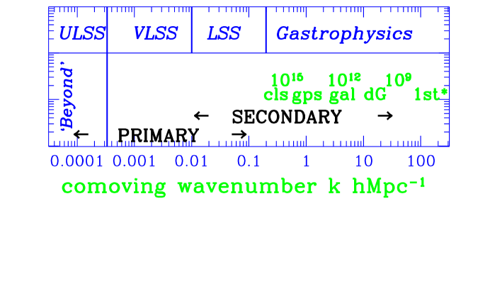
A theorist would argue that it is best to go for CMB probes, using spectacular forecasts [2, 3] of the percent level accuracy that cosmic parameters can be determined to because of the sensitive dependence of the anisotropies on the linear gas physics at photon decoupling at $z\sim 1000$. However, there are significant near-degeneracies among cosmological parameters such as $\Lambda$ and the curvature, which require other experiments, often wide-angle, to break. Further, to realize the promise will depend upon how well foreground signals from the Milky Way and secondary anisotropy signals from nonlinear phenomena such as the Sunyaev-Zeldovich effect from high pressure gas and emission from dusty high redshift galaxies can be disentangled from our goal, the primary anisotropies. CMB surveys can deliver useful information all the way from the ultralarge scale structure (ULSS) realm “beyond” (our Hubble patch) through the highly linear VLSS regime well-probed by COBE, into the LSS regime. We are now getting increasingly good LSS information from current small angle CMB anisotropy experiments (bandpower estimates shown in Fig. 3), we are about to take a significant step forward with balloon-borne and interferometer experiments, and a leap forward with the satellites MAP and Planck (lower right panel of Fig. 3).

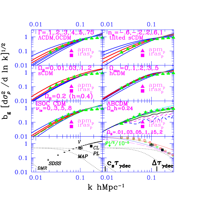
Galaxy redshift surveys probe number density fields, so they are largely limited to probing the LSS band since the level of mass density fluctuations is apparently rather tiny in the VLSS band. The further complication inherent in biasing relative to the mass density field may still obscure the derivation of the gravitational potential field. In Fig. 2, this unknown is absorbed in a uniform-amplifier bias factor $b_{g}$ which the simplest biasing theories predict in the linear regime, but which we know could be quite environment and scale dependent in a way which may make reliable calculations difficult.

We do think that for clusters the biasing has a simple physical explanation involving collapsed halos that allows for reliable calculations and extraction of the gravitational potential field from cluster surveys constructed using X-ray, optical or SZ data. It is this same simplicity of interpretation which has allowed the estimates of the mass power spectrum from cluster abundances (lower panels of Fig. 2).

It seems that practical limitations will limit weak gravitational lensing and large scale streaming velocities to the LSS regime, even though they are direct probes of $\Phi$ gradients.

The length scales below LSS, labelled “gastrophysics”, are ones over which energy injection and propagation, through ionization and shock fronts from galaxies, quasars, etc. are expected to have had important effects. That is, even if the dark matter density power in the $k$-bands in question (e.g., the galaxy band of Fig. 1 at $z\sim 4$) is linear, the gas effects can lead to severe and complex biasing or antibiasing over such scales. Thus, although probes based on wide field catalogues of high redshift galaxies and quasars, and on quasar absorption lines from the intergalactic medium, represent a very exciting observational frontier, it will be difficult for theoretical conclusions about the early universe and the underlying fluctuations to be divorced from these gastrophysical complications.

Figure 2: These panels show how the shape of the linear density power spectrum in the LSS regime changes as the cosmological model is varied. These are compared with the reconstructed linear power spectrum estimated by Peacock[4]. It is unclear how seriously the discrepencies above $0.1({\rm\,h^{-1}Mpc})^{-1}$ should be taken. The two lower panels show how strong the overlap will be between CMB and redshift surveys. Right focuses on ${\cal P}_{\rho}^{1/2}$, left on ${\cal P}_{\Phi}^{1/2}$. A forecast of error bars for the number density power spectrum derived from the SDSS by Vogeley and Szalay, and current mass density power spectrum estimates from cluster abundances ($CL$) and large scale streaming velocities ($V$), are contrasted with the dotted $k$-space filters for MAP and Planck. Planck in particular encompasses well the two important scales which define the effective acoustic peak range for primary anistropies (those involving linear fluctuations): the sound crossing distance $c_{s}\tau_{\gamma dec}$ at photon decoupling around redshift 1000; the width $\Delta\tau_{\gamma dec}$ of the region over which this decoupling occurs, which is about a factor of 10 smaller, and below which primary CMB anisotropies are damped. Estimates of the linear $\Phi$ power from current galaxy clustering data by [4] are compared with some sample (linear) COBE-normalized gravitational potential power spectra on the right. A bias is “allowed” to (uniformly) raise the shapes to match the observations.

1.1 Cosmic Structure and the Nonlinear Wavenumber

Various (linear) density power spectra, ${\cal P}_{\rho}(k)\propto k^{4}{\cal P}_{\Phi}(k)$, are shown in Fig. 2. Many people plot ${\cal P}_{\rho}/k^{3}\sim k{\cal P}_{\Phi}$ instead. Here ${\cal P}_{\Phi}(k)$ $\equiv d\sigma_{\Phi}^{2}/d\ln k$ is the rms power in each $d\ln k$ band. In hierarchical structure formation models such as those considered here, the nonlinear wavenumber $k_{NL}(t)$, defined by $\sigma_{\rho}(k_{NL})=1$, where $\sigma_{\rho}^{2}(k)\equiv\int_{0}^{k}{\cal P}_{\rho}(k)d\ln k$, grows as the universe expands. $k_{NL}(t)$ was in the galaxy band at redshift 3 and is currently in the cluster band.

At a given time $t$, there is a band in $k$ extending just above $k_{NL}(t)$ which is primarily responsible for the nonlinear collapsed dark matter halos in the medium in hierarchical theories. Smaller halos that formed earlier from much higher $k$ bands would have largely merged into the halos of relevance at epoch $t$, in a sequence of characteristic objects shown in Fig. 1. If we denote the rms linear density fluctuation level for waves longer than $k$ by $\sigma_{\rho}(k)$, then the characteristic scale $k_{*}$ which gives the peak of the Press-Schechter distribution of collapsed objects, $d\Omega_{coll}(M)/d\ln M$, occurs at $\sigma_{\rho}(k_{*})=f_{c}$, where $f_{c}$ is a suitable collapse threshold, the famous 1.686 for $\Omega=1$. Associated with $k_{*}$ is a characteristic mass $M_{*}$. On the other hand, for mass scales below $\sigma_{\rho}=f_{c}/3\approx 0.6$ not even $3\sigma$ peaks will have collapsed at this resolution. As we describe later, this is the weakly nonlinear domain of the cosmic web of interconnected structure: the view of the structure smoothed on these scales reveals the characteristic patterns of filaments connecting clusters, and membranes connecting filaments. Voids are rare density minima which have opened up by gravitational dynamics and merged, opposite to the equally abundant rare density maxima, the clusters, in which the space collapses by factors of 5-10 and more.

At $k>k_{NL}(t)$, nonlinearities and complications associated with dissipative gas processes can obscure the direct connection to the early universe physics. Indeed, the reason galaxies are still around today when $k_{NL}$ is cluster scale is that, although the outer halos of the galaxies will have largely merged, gas cooling allows the baryons and some of the dark matter to concentrate and survive as independent beings in groups and clusters, breaking the hierarchy.

Most easily interpretable are observables probing the linear regime now, $k<k_{NL}(t_{0})$. CMB anisotropies arising from the linear regime are termed primary; as Fig. 1 shows, these probe 3 decades in wavenumber, with the range defined by CMB damping rather than by any nonlinear effects at $z\sim 1000$. LSS observations at low redshift probe a smaller, but overlapping, range. We have hope that $z\sim 3$ LSS observations, when $k_{NL}(t)$ was larger, can extend the range, but gasdynamics can modify the relation between observable and power spectrum in complex ways. Secondary anisotropies of the CMB, those associated with nonlinear phenomena, also probe smaller scales and the “gastrophysical” realm.

1.2 Early Universe Connection and the Freedom in Inflation

The source of fluctuations to input into the cosmic structure formation problem is likely to be found in early universe physics. The contenders for generation mechanism are (1) “zero point” quantum noise in scalar and tensor fields that must be there in the early universe if quantum mechanics is applicable and (2) topological defects which may arise in the inevitable phase transitions expected in the early universe.

From CMB and LSS observations we hope to learn: the statistics of the fluctuations, whether Gaussian or non-Gaussian; the mode, whether adiabatic or isocurvature scalar perturbations, and whether there is a significant component in gravitational wave tensor perturbations; the power spectra for these modes, ${\cal P}_{\Phi}(k),{\cal P}_{is}(k),{\cal P}_{GW}(k)$ as a function of comoving wavenumber $k$. As the Universe evolves the initial shape of ${\cal P}_{\Phi}$ (nearly flat or scale invariant) is modified by characteristic scales imprinted on it that reflect the values of cosmological parameters such as the energy densities of baryons, cold and hot dark matter, in the vacuum (cosmological constant), and in curvature. Often observables can be expressed as weighted integrals over $k$ of the final state power specta and thus can probe both $\Omega$’s and initial power amplitudes and tilts.

Many variants of the basic inflation theme have been proposed, sometimes with radically different consequences for ${\cal P}_{\Phi}(k)\sim k^{1-n_{s}(k)}$, and thus for LSS, which is used in fact to highly constrain the more baroque models. The most likely inflation possibilities are the simplest: (1) adiabatic curvature fluctuations with nearly uniform scalar tilt over the observable range, slightly more power to large scales ($0.8\mathrel{\hbox to0.0pt{\lower 3.0pt\hbox{$\mathchar 536\relax$}\hss}\raise 2.0pt\hbox{$\mathchar 316\relax$}}n_{s}\mathrel{\hbox to0.0pt{\lower 3.0pt\hbox{$\mathchar 536\relax$}\hss}\raise 2.0pt\hbox{$\mathchar 316\relax$}}1$) than “scale invariance” ($n_{s}=1$) gives, a predictable nonzero gravity wave contribution with tilt similar to the scalar one, and tiny mean curvature ($\Omega_{tot}\approx 1$); (2) same as (1), but with a tiny gravity wave contribution.

An arguable rank-ordering of the more baroque inflation possibilities (see e.g., [1, 6] for references) is: (3) same as (1) but with a subdominant isocurvature component of nearly scale invariant tilt (the case in which isocurvature dominates is ruled out, but see Figs. 2,3); (4) radically broken scale invariance with weak to moderate features (ramps, mountains, valleys) in the fluctuation spectrum (strong ones are largely ruled out); (5) radical breaking with non-Gaussian features as well; (6) “open” inflation, with quantum tunneling or possibly a Hawking-Turok instanton resulting in a negatively-curved (hyperbolic) space which inflates, but not so much as to flatten the mean curvature; (7) quantum creation of compact hyperbolic space from “nothing”. It is quite debatable which of the cases beyond (2) are more or less plausible, with some claims that (4) is supersymmetry-inspired, others that (6) is not as improbable as it sounds.

1.3 Cosmic Parameters and the CMB

Even simple Gaussian inflation-generated fluctuations for structure formation have a large number of early universe parameters we would wish to determine: power spectrum amplitudes at some normalization wavenumber $k_{n}$ for the modes present, $\{{\cal P}_{\Phi}(k_{n}),{\cal P}_{is}(k_{n}),{\cal P}_{GW}(k_{n})\}$; shape functions for the “tilts” $\{\nu_{s}(k),\nu_{is}(k),\nu_{t}(k)\}$, usually chosen to be constant or with a logarithmic correction, e.g., $\nu_{s}(k_{n}),d\nu_{s}(k_{n})/d\ln k$. (The scalar tilt for adiabatic fluctuations, $\nu_{s}(k)\equiv d\ln{\cal P}_{\Phi}/d\ln k$, is related to the usual index, $n_{s}$, by $\nu_{s}=n_{s}-1$.) The transport problem is dependent upon physical processes, and hence on physical parameters. A partial list includes the Hubble parameter ${\rm h}$, various mean energy densities $\{\Omega_{tot},\Omega_{B},\Omega_{\Lambda},\Omega_{cdm},\Omega_{hdm}\}{\rm h}^{2}$, and parameters characterizing the ionization history of the Universe, e.g., the Compton optical depth $\tau_{C}$ from a reheating redshift $z_{reh}$ to the present. Instead of $\Omega_{tot}$, it is becoming conventional to use the curvature energy parameter, $\Omega_{k}\equiv 1-\Omega_{tot}$, thus zero for the flat case. In this space, the Hubble parameter, ${\rm h}=(\sum_{j}(\Omega_{j}{\rm h}^{2}))^{1/2}$, and the age of the Universe, $t_{0}$, are functions of the $\Omega_{j}{\rm h}^{2}$. The density in nonrelativistic (clustering) particles is $\Omega_{nr}=\Omega_{B}+\Omega_{cdm}+\Omega_{hdm}$, denoted as well by $\Omega_{m}$. The density in relativistic particles, $\Omega_{er}$, includes photons, relativistic neutrinos and decaying particle products, if any. $\Omega_{er}$, the abundance of primordial helium, etc. should also be considered as parameters to be determined. The count is thus at least 17, and many more if we do not restrict the shape of ${\cal P}_{\Phi}(k)$ through theoretical considerations of what is “likely” in inflation models. For example, the ratio of gravitational wave power to scalar adiabatic power is ${\cal P}_{GW}/{\cal P}_{\Phi}\approx-(100/9)\nu_{t}/(1-\nu_{t}/2)$, with small corrections depending upon $\nu_{s}-\nu_{t}$ [1]. If such a relationship is assumed, the parameter count is lowered by one, and other restrictions on most likely behaviour or prior probabilities reflecting other observations or prejudices are used to reduce the set further; e.g., the forecasts for the MAP and Planck satellites in [2] used a 9 parameter set.

For a given model, the early universe ${\cal P}_{\Phi}$ is uniquely related to late-time power spectrum measures of relevance for the CMB, such as the quadrupole or averages over $\ell$-bands, and to LSS measures, such as the rms density fluctuation level on the $8{\rm\,h^{-1}Mpc}$ (cluster) scale, $\sigma_{8}$, so any of these can be used in place of the primordial power amplitudes in the parameter set.

The arena in which CMB theory battles observation is the anisotropy power spectrum in multipole space, Fig. 3, which shows how primary ${\cal C}_{\ell}$’s vary with some of these cosmic parameters. Here ${\cal C}_{\ell}\equiv\ell(\ell+1){\langle|(\Delta T/T)_{\ell m}|^{2}\rangle}/(2\pi)$. Cosmological radiative transfer in the linear regime and therefore the ${\cal C}_{\ell}$ predictions as the cosmological parameters are varied is on a firm theoretical footing; for reviews, see [1, 8, 9]. The ${\cal C}_{\ell}$ sets shown correspond to those in Fig. 2. They also are chosen to have the fixed cosmological age of 13 Gyr, similar to that inferred from globular cluster ages. Bond and Jaffe [7] used all of the current CMB data to test such sets for tilted $\Lambda$CDM, h$\Lambda$CDM, oCDM sequences, with and without gravity wave contributions and wide variation in $\Omega_{\Lambda}$, $H_{0}$, $n_{s}$, etc. and for ages from 11 to 15 Gyr. Results quoted here on parameters from current CMB data and combining CMB and LSS data are from that work.

Figure 3: The ${\cal C}_{\ell}$ anisotropy bandpower data up to summer 1998 compressed to 9 bands using the methods of [5] are compared with various 13 Gyr model sequences (left to right): (1) $H_{0}$ from 50 to 90, $\Omega_{\Lambda}$, 0 to 0.87, for an untilted $\Lambda$CDM sequence; (2) $n_{s}$ from 0.85 to 1.25 for the $H_{0}=70$ $\Lambda$CDM model ($\Omega_{\Lambda}=.66$) – dotted is 0.85 with gravity waves, next without, upper dashed is 1.25, showing visually why $n_{s}$ is found to be unity to within 5%; (3) $\Omega_{B}{\rm h}^{2}$ from 0.003 to 0.05 for the $H_{0}=50$ sCDM model; (4) $H_{0}$=50 sequence with neutrino fractions varying from 0.1 to 0.95; (5) an isocurvature CDM sequence with positive isocurvature tilts ranging from 0 to 0.8; (6) $\Omega_{B}{\rm h}^{2}$ from 0.003 to 0.05 for the $H_{0}=70$ $\Lambda$CDM model; (7) $H_{0}$ from 50 to 65, $\Omega_{k}$ from 0 to 0.84 for the untilted oCDM sequence, showing the strong $\ell$-shift of the acoustic peaks with $\Omega_{k}$; (9) sample defect ${\cal C}_{\ell}$’s for textures, etc. from [15] – cosmic string ${\cal C}_{\ell}$’s from [16] are similar and also do not fare well compared with the current data. The bottom right panel is extended to low values to show the magnitude of secondary fluctuations from the thermal SZ effect for the $\Lambda$CDM model. The kinematic SZ ${\cal C}_{\ell}$ is significantly lower. Dusty emission from early galaxies may lead to high signals, but the power is concentrated at higher $\ell$, with a weak tail because galaxies are correlated extending into the $\ell\mathrel{\hbox to0.0pt{\lower 3.0pt\hbox{$\mathchar 536\relax$}\hss}\raise 2.0pt\hbox{$\mathchar 316\relax$}}2000$ regime. Forecasts of how accurate ${\cal C}_{\ell}$ will be determined for an sCDM model from MAP (error bars growing above $\ell\sim 700$) and Planck (small errors down the ${\cal C}_{\ell}$ damping tail) are also shown.

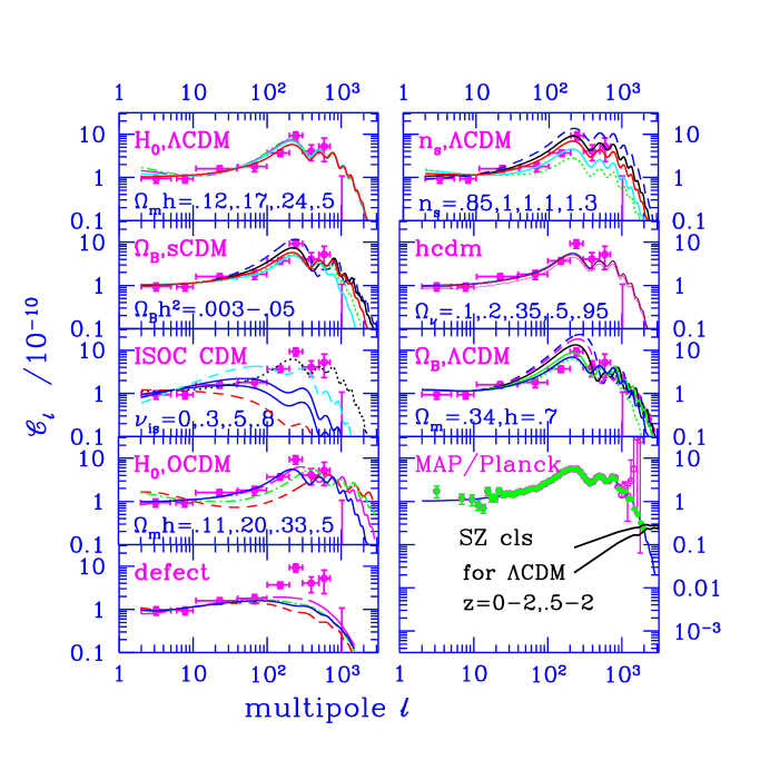
The ${\cal C}_{\ell}$’s are normalized to the 4-year dmr(53+90+31)(A+B) data, which fixes it to within about 7% in amplitude. DMR is fundamental to analyses of the VLSS region and ULSS region, and is the data set that is the most robust at the current time. Even with the much higher precision MAP and Planck experiments we do not expect to improve the results on the COBE angular scales greatly because the 4-year COBE data has sufficiently large signal-to-noise that one is almost in the cosmic variance error limit (due to realization to realization fluctuations of skies in the theories) which cannot be improved upon no matter how low the experimental noise.

The “beyond” land in Fig. 1 is actually partly accessible because ultralong waves contribute gentle gradients to our CMB observables. The DMR data is well suited to testing whether radical broken scale invariance results in a huge excess or deficit of power in the COBE $k$-space band, e.g., just beyond $k^{-1}\sim H_{0}^{-1}$, but this has not been much explored. The remarkable non-Gaussian structure predicted by stochastic inflation theory would likely be too far beyond our horizon for its influence to be felt in the DMR data. The bubble boundary in hyperbolic inflation models may be closer and its influence shortly after quantum tunneling occurred could possibly have observable consequences for the CMB. Theorists have also constrained the scale of topology in simple models. For compact spatial manifolds (which may have $\Omega\leq 1$ as well as $\Omega>1$), the wavenumbers have an initially discrete spectrum, and are missing ultralong waves, limited by the size of the manifold. Usually isotropy is radically broken in such models, resulting in CMB pattern formation which allows much stronger constraints to be imposed than results just from the lack of ULSS power; e.g., [11] find for flat equal-sided 3-tori, the inscribed radius must exceed $1.1(2H_{0}^{-1})=6600{\rm\,h^{-1}Mpc}$ from DMR at the $95\%$ confidence limit, with the weaker $>0.7(2H_{0}^{-1})$ constraint for asymmetric 1-tori. It is also not as strong if the platonic-solid-like manifolds of compact hyperbolic topologies are considered, though the overall size of the manifold should be at least of order the last scattering surface radius [11].

The primoridial spectral tilt $n_{s}$ is surprisingly well determined using CMB data alone, as the upper right panel of Fig. 3 suggests. If $\sigma_{8}$ is marginalized for the tilted $\Lambda$CDM sequence with $H_{0}$=50, with DMR only the primordial index is $n_{s}$ = $1.02^{+.23}_{-.25}$ with no gravity waves, $\nu_{t}$=0, and $1.02^{+.23}_{-.18}$ with gravity waves and $\nu_{t}$=$\nu_{s}$, rather encouraging for the nearly scale invariant models preferred by inflation theory. For the 13 Gyr tilted $\Lambda$CDM sequence, when all of the current CMB data are used [7] get $1.02^{+.05}_{-.03}$ for $H_{0}=50$ (and $\Omega_{\Lambda}=0$, the tilted sCDM model sequence) and $1.00^{+.04}_{-.04}$ for $H_{0}=70$ (and $\Omega_{\Lambda}=0.66$). Marginalizing over $H_{0}$ gives $1.01^{+.05}_{-.04}$ with gravity waves included, $0.98^{+.08}_{-.06}$ if they are not. The marginalized 13 Gyr tilted oCDM sequence gives $1.00^{+.05}_{-.05}$.

Constraints on such “global parameters” as average curvature, $H_{0}$ and $\Omega_{\Lambda}$ from COBE data alone are not very good, and the situation for the $\Lambda$CDM sequences is not that much improved with all of the CMB data. After marginalizing over all $n_{s}$, [7] get $H_{0}<75$ at $1\sigma$, but effectively no constraint at 2$\sigma$. The strong dependence of the position of the acoustic peaks on $\Omega_{k}$ means that the oCDM sequence is better restricted: $\Omega_{tot}\sim.7$ is preferred; for the 13 Gyr sequence this gives $H_{0}\approx 53$ and for the 11 Gyr sequence $H_{0}\approx 65$.

1.4 Cosmic Parameters and LSS (+CMB)

We have always combined CMB and LSS data in our quest for viable models. DMR normalization determines $\sigma_{8}$ to within 7%, and comparing with the $\sigma_{8}\sim 0.6\Omega_{nr}^{-0.56}$ target value derived from cluster abundance observations severely constrains the cosmological parameters defining the models. In Fig. 2, this means the COBE-normalized ${\cal P}_{\Phi}(k)$ must thread the “eye of the needle” in the cluster-band.

Similar constrictions arise from galaxy-galaxy and cluster-cluster clustering observations: the shape of the linear ${\cal P}_{\rho}$ must match the shape reconstructed from the data. The one plotted in the panels of Fig. 2 is from [4]. The clustering observations are roughly compatible with an allowed range $0.15\mathrel{\hbox to0.0pt{\lower 3.0pt\hbox{$\mathchar 536\relax$}\hss}\raise 2.0pt\hbox{$\mathchar 316\relax$}}\Gamma+\nu_{s}/2\mathrel{\hbox to0.0pt{\lower 3.0pt\hbox{$\mathchar 536\relax$}\hss}\raise 2.0pt\hbox{$\mathchar 316\relax$}}0.3$, where the oft-used $\Gamma=\Gamma_{eq}\,e^{-(\Omega_{B}(1+\Omega_{nr}^{-1}(2{\rm h})^{1/2})-0.06)}$, $\Gamma_{eq}\approx\Omega_{nr}\,{\rm h}\,[\Omega_{er}/(1.68\Omega_{\gamma})]^{-1/2}$, characterizes the density transfer function shape. The reason $\Gamma_{eq}$ looms so large is that it parameterizes the scale of the horizon when the energy density in nonrelativistic and relativistic matter are the same, $k_{Heq}^{-1}=5\,\Gamma_{eq}^{-1}{\rm\,h^{-1}Mpc}$. The sCDM model with $\Omega_{B}=0.03$ has $\Gamma\approx 0.5$. The phenomenological $\Gamma/\Gamma_{eq}$ correction factor cannot fully parameterize the effects of increasing $\Omega_{B}$ on the power spectrum, which has the “Sakharov oscillations” evident in Fig 2 in the $\Lambda$BCDM models.

To get $\Gamma+\nu_{s}/2$ in the observed range one can: lower ${\rm h}$, lower $\Omega_{nr}$ ($\Lambda$CDM, oCDM), raise $\Omega_{er}$, the density parameter in relativistic particles ($1.68\Omega_{\gamma}$ with 3 species of massless neutrinos and the photons), e.g., as in $\tau$CDM, with a decaying $\nu$ of lifetime $\tau_{d}$ and $\Gamma\approx 1.08\Omega_{nr}{\rm h}(1+0.96(m_{\nu}\tau_{d}/{\rm keV~{}yr})^{2/3})^{-1/2}$; raise $\Omega_{B}$; tilt $\nu_{s}<0$, e.g., for sCDM parameters $0.3\mathrel{\hbox to0.0pt{\lower 3.0pt\hbox{$\mathchar 536\relax$}\hss}\raise 2.0pt\hbox{$\mathchar 316\relax$}}n_{s}\mathrel{\hbox to0.0pt{\lower 3.0pt\hbox{$\mathchar 536\relax$}\hss}\raise 2.0pt\hbox{$\mathchar 316\relax$}}0.7$ would be required. Adding a hot dark matter component gives a power spectrum characterized by more than just $\Gamma$ since the neutrino damping scale enters as well as $k_{Heq}$, as is clear from Fig. 2. In the post-COBE era, all of these models that lower $\Gamma+\nu_{s}/2$ have been under intense investigation to see which survive as the data improves, if any.

The deviation in the shape derived using the APM data [4] from the simple $\Gamma$ law form may require more baroque models, such as tilted h$\Lambda$CDM models (see e.g., [10, 7]).

Combining LSS and all CMB data gives more powerful discrimination among the theories. The approach [7] used to add LSS information to the CMB likelihood functions was to design prior probabilities for $\Gamma+\nu_{s}/2$ and $\sigma_{8}\Omega_{nr}^{0.56}$, reflecting the current observations, but with flexible and generous non-Gaussian and asymmetric forms to ensure the priors can encompass possible systematic problems in the LSS data. For example, their choice for $\sigma_{8}\Omega_{nr}^{0.56}$ was relatively flat over the 0.45 to 0.65 range.

Using all of the current CMB data and the LSS priors, for the 13 Gyr $\Lambda$CDM sequence with gravity waves included, [7] get $n_{s}=1.00^{+.05}_{-.03}$ and $H_{0}=72\pm 3$ ($\Omega_{\Lambda}\approx 0.7$), respectively, when $H_{0}$ and $n_{s}$ are marginalized; with no gravity waves, $0.96^{+.07}_{-.05}$ and $H_{0}=70\pm 3$ are obtained; and for an h$\Lambda$CDM sequence, with a fixed ratio $\Omega_{hdm}/\Omega_{nr}=0.2$ for two degenerate massive neutrino species, $n_{s}\approx 0.97^{+.02}_{-.02}$ and $H_{0}\approx 57^{+5}_{-3}$ are obtained, revealing a slight preference for $\Omega_{\Lambda}\sim 0.3$. A slight increase in age above 13 Gyr lowers $H_{0}$ to the perhaps more preferable 65.

For the 13 Gyr oCDM sequence, best fit CMB-only models have $\sigma_{8}$ too low compared with the cluster abundance requirements, so the joint CMB+LSS maximum likelihood is substantially below that for $\Lambda$CDM, and severely challenged by the data just as it is for the SNIa data.

The isocurvature CDM models with tilt $\nu_{is}>0$, e.g., [12, 13], can more or less fit the ${\cal P}_{\rho}$ shape data in Fig. 2, but are certainly challenged by the current CMB data in Fig. 3. $\Lambda$BCDM models with an increasing value of $\Omega_{B}$ do have problems with the CMB data, but it can be partly overcome with tilt; the deviations in the ${\cal P}_{\rho}$ shape from the observed are rather too pronounced though (e.g., [14]). Calculations of defect models (e.g. strings and textures) give ${\cal C}_{\ell}$’s that do not have the prominent peak that the data seem to indicate [15, 16], as Fig. 3 shows. These are only a few of the many examples in which the CMB+LSS data has already narrowed our attention enormously in structure formation model space.

2 Nonlinear Probes

We have mentioned that the magnitude of the linear $\sigma_{\rho}(k)$ is a good monitor of the sort of dynamics at the resolution that the $k$-scale defines. For $\sigma_{\rho}(k)\mathrel{\hbox to0.0pt{\lower 3.0pt\hbox{$\mathchar 536\relax$}\hss}\raise 2.0pt\hbox{$\mathchar 316\relax$}}0.1$ we are solidly in the linear regime. The weakly nonlinear regime between 0.1 and $\sigma_{\rho}\sim 0.7$ defines the $k$-band largely responsible for the cosmic web, while the regime between 0.7 and 2 encompasses most of the virialized objects.

Over time there have been a number of approximation techniques proposed to mimic LSS dynamics. They usually involve the weakly nonlinear regime and were designed to be significantly faster than the full $N$-body calculations. However, with the advent of very fast computing, unless they had some sort of semi-analytic counterpart to enhance the depth of understanding such techniques are of ever-diminishing importance. The most venerable and still useful is the Zeldovich approximation, i.e., first order Lagrangian perturbation theory. Second order Lagrangian perturbation theory is much more accurate, but also harder to implement. The Zeldovich approximation with sticking at caustic formation is called adhesion theory [18], utilizing Burgers equation for the velocity. It successfully describes the architecture of voids, filaments and clusters but does not deal with interior dynamics of “stuck structure” and has not been very useful for mass estimates. The frozen potential and frozen flow approximations are attempts to avoid full potential calculations, but are instrinsically numerical, and do not work that well. See [19] for a review.

What has been applied with great success is weakly nonlinear perturbation theory, both Eulerian and Lagrangian, much of it by our French hosts (see e.g., [20]). Some of the milestones in this effort are: accurate prediction of the one-point distribution function (PDF) for the overdensity $\delta$ at “tree level” c.f. N-body results [21, 22]; analytic expressions for the cumulants $S_{n}={\langle\delta^{n}\rangle}/(\sigma_{\rho,NL}^{2})^{n-1}$ to “tree order” $S_{n}\sim{\cal O}(\sigma_{\rho}^{2n-2})$ agree well with $N$-body results [23]; calculation of the variance ${\langle\delta^{2}\rangle}=\sigma_{\rho,NL}^{2}$ to “one-loop” order [24, 25] and, in a tour de force, $S_{3}$ [26] and the bispectrum [27] to this order (the $\sigma_{\rho,NL}^{2}$ order correction to the tree level results).

As one heads into somewhat stronger nonlinearity, $\sigma_{\rho}\mathrel{\hbox to0.0pt{\lower 3.0pt\hbox{$\mathchar 536\relax$}\hss}\raise 2.0pt\hbox{$\mathchar 318\relax$}}0.7$, analytic methods to deal with object collapse are heavily utilized. The hugely popular, trivial-to-implement, Press-Schechter (1976) method, as modified by [35] to the excursion set theory: at each point in space, $\delta_{L}(k)$ is allowed to random walk as the resolution $\sigma_{\rho}$ increases, i.e., as the scale $k^{-1}$ decreases. Once the $\delta_{L}(k)$ reaches a redshift-dependent threshold $f_{c}(z)$, the “absorbing barrier”, that point is said to have collapsed at that redshift and is assigned to a halo with mass $M$ corresponding to the scale $k$. The flaw [35] is evident: nearby points that belong to the same halo will be assigned to different mass objects. Thus the amazement, and delight, in the community that the one-point distribution, $n(M)d\ln M$, so derived fits that of $N$-body group catalogues so well [35, 36, 34], even below $M_{*}$. So do such interesting constrained mass functions as $n(M_{2},z_{2}|M_{1},z_{1})$ giving the number density of objects of mass $M_{2}$ at redshift $z_{2}$ given that the region is already within one of mass $M_{1}$ at redshift $z_{1}$.

The peak-patch picture [34] described below is the natural generalization of the Press-Schechter method to include non-local effects, spatial correlations and more natural ways of assigning mass to halos. It is also the natural generalization of BBKS single-filter peaks theory [37] to allow a mass spectrum and solve the cloud-in-cloud (i.e., peak-in-peak) problem. In it, the threshold $f_{c}$ becomes a function of the tidal environment the peak patch finds itself in. It is also at the heart of our cosmic web picture.

Another approach to the nonlinear evolution of ${\cal P}_{\rho}(k)$ is that of Hamilton et al. [28], where a Lagrangian wavenumber $k_{L}$ of linear theory is mapped onto a nonlinear wavenumber $k_{NL}$ through $k_{NL}^{-1}\approx(1+\overline{\delta}_{NL})^{-1/3}k_{L}^{-1}$, where $\overline{\delta}_{NL}$ is the average nonlinear overdensity in a mean field region of scale $k_{NL}^{-1}$, just what you would expect if you took a spherical Lagrangian radius and compressed it to an Eulerian radius while conserving the mass. A mapping from the linear power spectrum ${\cal P}_{\rho L}$ to the nonlinear is defined by ${\cal P}_{\rho NL}(k_{NL})={\tt fn}({\cal P}_{\rho L}(k_{L}))$, where ${\tt fn}$ denotes a suitably fit nonlinear function, which, however, is dependent upon the shape of the linear power spectrum [29]. The VIRGO consortium tested the fn fit given by [30] with their $N$-body runs, and find accurate mapping from ${\cal P}_{\rho L}$ to power levels ${\cal P}_{\rho NL}$ up to $\sim 1000$. It was used by [4] to take the nonlinear galaxy power spectrum derived e.g., from the APM survey and make an estimate of the linear one: this is what we adopted for comparing with theory in Fig. 2.

There is of course the direct numerical approach to nonlinear physics. We describe the various $N$-body and hydro methods currently employed in cosmology. We then turn our attention to the peak-patch picture and the cosmic web.

2.1 N-Body and Gas Simulations

The ITP Cluster Comparison of Cosmological Hydro Codes was a “homework problem” assigned to simulators at the extended workshop on Galaxy Formation and Cosmic Radiation Backgrounds held at the Institute for Theoretical Physics in Santa Barbara in 1995. Calculations were finished in 1996/97 and the paper was submitted in 1998 [31]. A constrained single peak field was used for initial conditions to ensure that a massive COMA-like cluster would form at the centre of the simulation. The results provide a good snapshot of the $N$-body and hydro methods currently in use in cosmology, although improvements in all of the codes have been made since the test. The people participating and the codes used are listed in Table 2.1.

ITP Cluster Comparison of Cosmological Hydro+N-body Codes [31] Group Method CPU machine storage Bond & Wadsley SPH+P³MG 119hr DEC$\alpha$ 100MB Bryan & Norman PPM+PM 200 SGI PowCh 500 Cen TVD+PM 5312 IBM Sp2 4400 Evrard SPH+P³M 320 HP375 17 Gnedin SLH+P³M 136 SGI PowCh 90 Jenkins, Thomas & Pearce SPH+AP³M 5000 Cray-T3D 512 Owen & Villumsen ASPH+PM 40 Cray-YMP 106 Navarro SPH+Direct 120 Sparc10+Grape 75 Pen MMH+MMPM 480 SGI PowCh 900 Steinmetz SPH+Direct 28 Sparc10+Grape 22 Couchman SPH+AP³M 77 DEC$\alpha$ 95 Yepes & Klypin FCT+PM 350 Cray-YMP 480 Warren & Zurek Tree 15360 Intel-$\Delta$ 1000

GRAVITY SOLVERS: Direct refers to the brute force direct sum over all pairs to get the force. Tree refers to organizing distant particles into groups using a tree. PM refers to particle-mesh, using an FFT to compute the gravitational potential. MMPM is PM with a Lagrangian mesh distorted to move with the flow. P³M refers to particle-particle + PM, using FFTs to get the large scale force, and direct sum to get the small range force. AP³M is P³M with adaptive mesh refinement, so not as much costly P-P is needed. The preferred method of Bond & Wadsley is treeP³M, PM [38] for long-range forces with a tree-like P-P for the short-range. It is twice faster than the SPH-P³MG code used in our cluster comparison, with more accurate forces and half the storage requirement. (P³MG refers to particle-particle plus a multigrid solution to the Poisson equation to get the long range force.) Warren and Zurek did DM only, but a very large massively parallel benchmark calculation.

LAGRANGIAN HYDRO SOLVERS: These methods have resolution following the flow, hence increasing in high densityregions. SPH is Monaghan’s smooth particle hydrodynamics with spatially variable resolution; ASPH is aspherical SPH, using anisotropic kernels to treat asymmetric collapses better; MMH is moving-mesh hydro using a pseudo-Lagrangian grid-based technique; SLH is grid-based softened Lagrangian hydro. The Jenkins et al. simulation was a highly parallelized calculation using the SPH code Hydra; Couchman used it on a serial machine.

EULERIAN GRID-BASED HYDRO SOLVERS: PPM is the piecewise parabolic method; TVD refers to the Total Variation Diminishing hydro scheme; FCT refers to the Flux-Corrected-Transport scheme. For these Eulerian schemes to ultimately be effective in such compressible media as we deal with in cosmology, AMR (adaptive mesh refinement) must be used, which the PPM code has (an early single AMR version was used).

In spite of the huge variation in code types, CPU hours devoted, memory required, mass resolution and spatial resolution used, there was surprisingly good agreement among the calculations: excellent in the densities of gas and dark matter; good in the gas temperature, entropy, pressure, X-ray luminosity density, and gas to dark matter ratio; not as good in the highly dynamical earlier phases before cluster virialization.

The largest N-body simulation to date has been done by the VIRGO consortium, 1 billion particles using a P³M code of a periodic region $(2000{\rm\,h^{-1}Mpc})^{3}$ in size, on a CRAY T3E with 512 CPUs, of a $\Gamma=0.21$, $\sigma_{8}=0.6$ $\tau$CDM model. The mass resolution defined by the mass per particle was $4\times 10^{12}{\rm\,M_{\odot}}$ and the gravitational softening was $200{\rm\,kpc}$, chosen to ensure a do-able calculation by avoiding a large P-P slowdown. The texture of the cosmic web is very evident in the results [40].

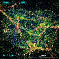
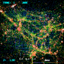
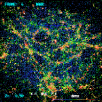
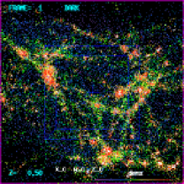
We have adopted a different approach we refer to as importance sampling [32], in which we do a number of simulations of constrained field initial conditions, chosen to sample most efficiently the statistical distribution of whatever quantities we wish to probe. It is as if we do a big-box simulation, and go around sampling this patch and that until we get statistical convergence. From this point of view, the big box simulations oversample the patches with large scale fluctuations near the rms, yet may undersample the rare protosupercluster or protosupervoid regions. If the periodic simulation volumes are not big enough so that there is negligible density power on the scale of the fundamental mode, $k^{-1}=L/(2\pi)$, then the big-box results will be in error. This is not a problem for the VIRGO simulation, but is a major headache for simulations of the Lyman $\alpha$ forest where $\sigma_{\rho}(k)$ changes slowly, and even more so for simulations of the “1st *” region. We design our simulation patches to avoid this [41]. For many purposes, we have found it adequate to calculate “shearing patches”, constrained by specifying the tidal tensor $\Phi_{,ij}$ at the origin smoothed on a few scales. However, we also may be interested in simulating complex regions, where more controlling constraints are used, e.g., associated with many cluster-scale density peaks. Our example of a dense supercluster is of this form.

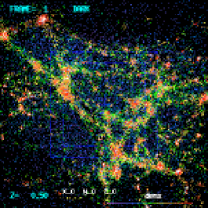
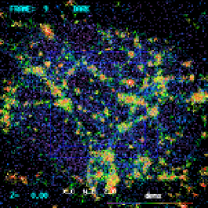
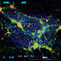
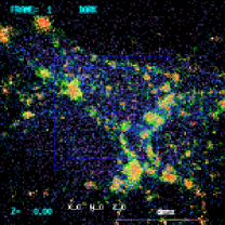
We now describe some aspects of simulation design. We first decide on the mass resolution we wish to achieve. This is set by the lattice spacing of particles on the initial high resolution grid, $a_{L}$, chosen to be $\sim 2{\rm\,Mpc}$ to ensure that the waves needed to treat the target objects forming in the simulation will be adequate, in this case clusters. Next we need to determine the spatial resolution, of the gas and of the gravitational forces, preferably highly linked. In Lagrangian codes like we use, this varies considerably, being very high in cluster cores, moderate in filaments, and not that good in voids. Here we wanted to get good calculations of the cluster cores, so we wanted our resolution to be in excess of $\sim 40{\rm\,kpc}$, and the value we get is about $30{\rm\,kpc}$. Given the target resolution, we then have to determine how large the high resolution part of the simulation volume is by CPU limitations on the number of particles we can run in the desired time. This may mean the high resolution volume may distort considerably during the simulation. To combat this, layers are added of progressively lower resolution volumes, to ensure accurate large scale tides/shearing fields operate on the high resolution patch. For the calculations shown, the High Resolution region of interest (grid spacing $a_{L}$, $50^{3}$ sphere) sits within a Medium Resolution region ($2\,a_{L}$, $40^{3}$), in turn within a Low Resolution region ($2\,a_{L}$, $32^{3}$). The mean external tide of the entire patch is linearly evolved and applied during the calculation.

Thus our sample simulation has a high resolution 104 Mpc diameter patch with $50^{3}/2$ gas and $50^{3}/2$ dark matter particles (initial grid spacing of 100 comoving kpc), surrounded by gas and dark particles with 8 times the mass to 166 Mpc, in turn surrounded by “tidal” particles with 64 times the mass to 266 Mpc. Bigger calculations are easily do-able without resorting to massive parallelization; e.g., a $100^{3}/2$ gas and $100^{3}/2$ dark matter particle calculation with a total of 1.6 million particles including the medium and low resolution regions takes about two weeks of SGI Origin 2000 single processor time.

The mass resolution limits the high $k$ power of the waves that can be laid down in the initial conditions (Nyquist frequency, $\pi/a_{L}$), but for aperiodic patches there is no constraint at the low $k$ end: we use the FFT for high $k$, but a power law sampling for medium $k$, and a log $k$ sampling for low $k$, the latter two done using SlowFT, i.e., a direct sum over optimally-sampled $k$ values, with the shift from one type of sampling to another determined by which gives the minimum volume per mode in $k$-space. By contrast, the periodic big box calculations are limited by the fundamental mode.

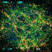
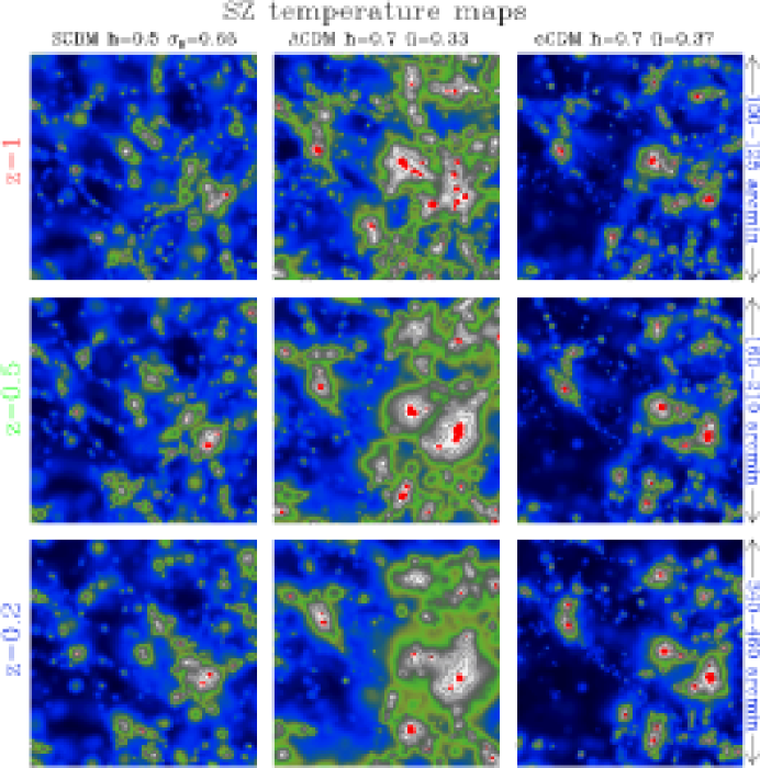
The numerical method we adopt is the cosmological SPH+treeP³M code of Wadsley and Bond [41]. The treeP³M technique is a fast, flexible method for solving gravity and can accurately treat free boundary conditions. The code includes photoionization as well as shock heating and cooling with abundances in chemical (but not thermal) equilibrium, incorporating all radiative and collisional processes. The species we consider are H, H⁺, He, He⁺, He⁺⁺ and e^-. The simulations were run from $z=30$ to $z=0$. Parameters for the sCDM, $\Lambda$CDM and oCDM cosmologies we have run are given in Fig. 4.

Our $a_{L}$ resolution is 2 times better than the VIRGO simulation, and our best spatial resolution is 6 times better. On the other hand, we are simulating only $10^{-5}$ of the VIRGO volume at high res: even with clever sampling, being computer-cheap does have its drawbacks; though this is a rare event, about a thousand similarly compact superclusters would be within the VIRGO volume. We are now running simulations at twice the resolution to ensure accuracy for X-ray emission in the filaments, not just in the clusters. Our resolution is adequate for making predictions for signals from the supercluster complex in the Sunyaev-Zeldovich effect (Fig. 5) and gravitational lensing (described in our companion paper [39]).

Figure 4: COMPACT SUPERCLUSTERS: Dark matter density in a patch $\sim 100{\rm\,Mpc}$ (comoving diameter) across at redshifts $z$=1, 0.5 and 0 (from top to bottom) of three constrained-field supercluster simulations with differing cosmologies, with HR region $104{\rm\,Mpc}$, MR region $166{\rm\,Mpc}$ and LR region $266{\rm\,Mpc}$, with wave coverage to $k^{-1}=1000{\rm\,Mpc}$, the very long waves entering through a self consistent mean tidal field. The cosmologies shown from left to right are standard CDM ($\sigma_{8}$=0.67, ${\rm h}$=0.5), $\Lambda$ĆDM ($\sigma_{8}$=0.91, ${\rm h}$=0.7, $\Omega_{nr}$=0.3349) and an Open CDM model ($\sigma_{8}$=0.91, ${\rm h}$=0.7, $\Omega_{nr}$=0.3689). The initial conditions were constructed using constraints from the peak patches either within the region or those exerting a significant tidal force on it. e.g., 17 peak patches (found at $z=0$ in a $400{\rm\,Mpc}$ simulation) were used for sCDM. The constraints imply the simulations have similar, though not identical, patterns. Whereas the middle panel $\Lambda$CDM simulation had 29, 10 and 2 clusters with mass above $3\times 10^{14}{\rm\,M_{\odot}}$ at redshift 0, 0.5 and 1 and oCDM had 20, 12 and 5, sCDM had 13, 3 and none, a dramatic statement of the very different redshift evolution of the cluster system for sCDM.

Figure 5: SUNYAEV-ZELDOVICH MAP for the supercluster region seen at redshifts 1, 0.5 and 0.2 subtending the angles shown. The observing wavelength was taken to be in the Rayleigh-Jeans region of the spectrum (so $\Delta T/T=-2y$ here). The core red regions are above $32\times 10^{-6}$, and the dark contours surrounding the white are at $2\times 10^{-6}$. These levels are now accessible to ground based instrumentation. Blank field SZ surveys using interferometers and bolometer experiments promise to revolutionize our approach to the cluster system, especially at $z\mathrel{\hbox to0.0pt{\lower 3.0pt\hbox{$\mathchar 536\relax$}\hss}\raise 2.0pt\hbox{$\mathchar 318\relax$}}0.5$. Although the contours do go into the far field of the cluster region because they probe the electron pressure, one needs to go below $10^{-6}$ to fully detect the filaments. The effect is more pronounced in the $\Lambda$CDM and $o$CDM universes than in the sCDM model. The analogue of this figure in weak lensing is shown in [39].

2.2 The Peak-Patch Picture and the Cosmic Web

We approach the connected ideas we loosely call Cosmic Web theory (Bond, Kofman and Pogosyan 1996, BKP) and the Peak-Patch Picture (Bond and Myers 1996, BM, where detailed references to the pre-1995 work quoted here are given) through a historical path that includes an outline of the relevant terminology. In 1965, Lin, Mestel & Shu showed that a cold triaxial collapse implied an oblate “pancake” would form. In 1970, Zeldovich developed his famous approximation and argued that pancakes would be the first structures that would form in the adiabatic baryon-dominated universes popular at that time. Generally for a cold medium, there is a full non-linear map: ${\bf x}({\bf r},t)\equiv{\bf r}-{\bf s}({\bf r},t)$, from Lagrangian (initial state) space, ${\bf r}$, to Eulerian (final state) space, ${\bf x}$. The map becomes multivalued as nonlinearity develops in the medium. It is conceptually useful to split the displacement field, ${\bf s}={\bf s}_{b}+{\bf s}_{f}$, into a smooth quasilinear long wavelength piece ${\bf s}_{b}$ and a residual highly nonlinear fluctuating field ${\bf s}_{f}$. As we have discussed, if the rms density fluctuations smoothed on scale $R_{b}$, $\sigma_{\rho}(R_{b})$, are $<{\cal O}(1/2)$, the ${\bf s}_{b}$-map is one-to-one (single-stream) except at the rarest high density spots. In the peak-patch approach, $R_{b}$ is adaptive, allowing for dynamically hot regions like protoclusters to have large smoothing and cool regions like voids to have small smoothing. If $D(t)$ is the linear growth factor, then ${\bf s}_{b}=D(t){\bf s}_{b}({\bf r},0)$ describes Lagrangian linear perturbation theory, i.e. the Zeldovich approximation. The large scale peculiar velocity is ${\bf V}_{Pb}=-\bar{a}(t)\dot{{\bf s}}_{b}({\bf r},t)$. What is important for us is the strain field (or deformation tensor):

$$e_{b,ij}({\bf r})\equiv-{1\over 2}\big{(}{\partial s_{bi}\over\partial r_{j}}+{\partial s_{bj}\over\partial r_{i}}\big{)}({\bf r})=-\sum_{A=1}^{3}\lambda_{vA}{\hat{n}}_{vA}^{i}{\hat{n}}_{vA}^{j},{\rm~{}where}$$

$$\ \lambda_{v3}={\delta_{Lb}\over 3}(1+3e_{v}+p_{v}),\ \lambda_{v2}={\delta_{Lb}\over 3}(1-2p_{v}),\ \lambda_{v1}={\delta_{Lb}\over 3}(1+3e_{v}-p_{v}),$$

and $\delta_{Lb}=-e_{b,i}^{i}$ is the smoothed linear overdensity, which we often express in terms of the height relative to the rms fluctuation level $\sigma_{\rho}(R_{b})$, $\nu_{b}\equiv\delta_{Lb}/\sigma_{\rho}(R_{b})$. The deformation eigenvalues are ordered according to $\lambda_{v3}\geq\lambda_{v2}\geq\lambda_{v1}$ and ${\hat{n}}_{vA}$ denote the unit vectors of the principal axes. In that system, $x_{A}=r_{A}(1-\lambda_{vA}({\bf r},t))$ describes the local evolution.

The strain tensor is related to the peculiar linear tidal tensor by ${\partial^{2}\Phi\over\partial x^{i}\partial x^{j}}=-4\pi G{\bar{\rho}}_{nr}\bar{a}^{2}\,e_{b,ij}$, where $\Phi$ is the peculiar gravitational potential, and to the linear shear tensor by the time derivative ${\dot{e}}_{b,ij}$. The anisotropic part of the shear tensor has two independent parameters, the ellipticity $e_{v}$ (always positive) and the prolaticity $p_{v}$.

Doroshkevich (1973) and later Doroshkevich & Shandarin (1978) were among the first to apply the statistics of Gaussian random fields to cosmology, in particular of $\lambda_{vA}$, at random points in the medium (see also [39]). Arnold, Shandarin and Zeldovich (1982) made the important step of applying the catastrophe theory of caustics to structure formation. This work suggested the following formation sequence: pancakes first, followed by filaments and then clusters. This should be compared to the BKP Web picture formation sequence: clusters first, followed by filaments and then walls. BKP also showed that filaments are really ribbons, walls are webbing between filaments in cluster complexes, and that walls are not really classical pancakes. For the Universe at $z\sim 3$, massive galaxies play the role of clusters, and for the Universe at $z\sim 5$ more modest dwarf galaxies take on that role.

The Web story relies heavily upon the theory of Gaussian random fields as applied to the rare “events” in the medium, e.g., high density peaks. Salient steps in this development begin with BBKS (1986) [37], where the statistics of peaks were applied to clusters and galaxies, e.g., the calculation of the peak-peak correlation function, $\xi_{pk,pk}$. In a series of papers, Bond (1986-90) and Bond & Myers (1990-93) developed the theory so that it could calculate the mass function, $n(M)d\ln M$. It was also applied to the study of how shear affects cluster alignments (e.g., the Binggeli effect), and to Ly$\alpha$ clouds, ‘Great Attractors’, giant ‘cluster-patches’, galaxy, group and cluster distributions, dusty PGs, CMB maps and quasars. This culminated in the BM “Peak-Patch Picture of Cosmic Catalogues”.

We briefly describe the BM peak-patch method and how it is applied to initial conditions for simulations such as in Fig. 4. We identify candidate peak points using a hierarchy of smoothing operations on the linear density field $\delta_{L}$. To determine patch size and mass we use an ellipsoid model for the internal patch dynamics, which are very sensitive to the external tidal field. A byproduct is the internal (binding) energy of the patch and the orientation of the principal axes of the tidal tensor. We apply an exclusion algorithm to prevent peak-patch overlap. For the external dynamics of the patch, we use a Zeldovich-map with a locally adaptive filter ($R_{pk}$) to find the velocity ${\bf V}_{pk}$ (with quadratic perturbation theory corrections sometimes needed). The peaks are rank-ordered by mass (or internal energy). Thus, for any given region, we have a list of the most important peaks. By using the negative of the density field, we can also get void-patches.

The peak-patch method allows efficient Monte Carlo constructions of 3D catalogues; gives very good agreement with $N$-body groups; has an accurate analytic theory with which to estimate peak properties, (e.g., mass and binding energy from mean-profiles, using $f_{c}(e_{v})$, $\langle{e_{v}|\nu_{pk}\rangle}$); and handles merging, with high redshift peaks being absorbed into low redshift ones.

Figure 6: These plots illustrate the molecular picture of large scale structure, with “bonds” bridging clusters. The initial conditions have been smoothed and Zeldovich-mapped. (Full $N$-body maps look similar.) Upper panels show a two-point mean field $\langle\delta_{L}|2$pks$\rangle$ constrained by two oriented clusters separated by $40{\rm\,h^{-1}Mpc}$, fully aligned and partially aligned. The next 4 panels show three-point and four-point mean fields for different peak-patch orientations taken from a simulation. Notice the lower density contrast webbing between the filaments. One of the supercluster simulations had initial conditions constrained by the clusters in this region.

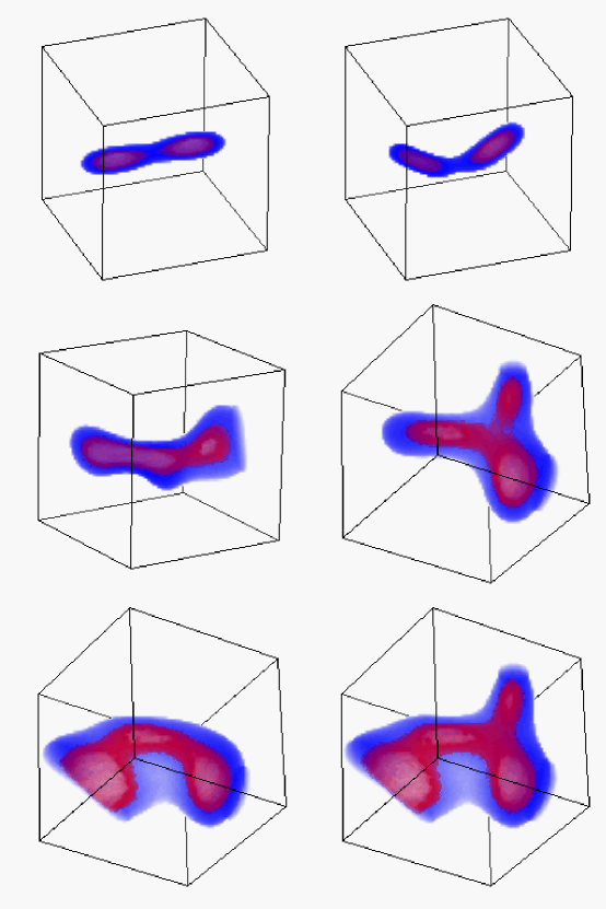
BKP concentrated on the impact the peak-patches would have on their environment and how this can be used to understand the web. They showed that the final-state filament-dominated web is present in the initial conditions in the $\delta_{Lb}$ pattern, a pattern largely determined by the position and primordial tidal fields of rare events. BKP also showed how 2-point rare-event constraints define filament sizes (see Fig. 6). The strongest filaments are between close peaks whose tidal tensors are nearly aligned, a binary molecule image with oriented peak-patches as the atoms. Strong filaments extend only over a few Lagrangian radii of the peaks they connect. They are so visually impressive in Eulerian space because the peaks have collapsed by about 5 in radius, leaving the long bridge between them, whose transverse dimensions have also decreased. The reason for the strong filaments between aligned peaks is that the high degree of constructive interference of the density waves required to make the rare peak-patches, and to preferentially orient them along the 1-axis, leads to a slower decoherence along the 1-axis than along the others, and thus a higher density. Membrane walls are the less dense webbing between the filaments, a $3,4,\ldots$-peak molecular image, also shown in Fig. 6. And void-patches are the inverse of peak-patches in the initial conditions, but mapped by nonlinear dynamics into the dominant volume elements.

The Cosmic Web and Peak-Patch pictures provide powerful language for understanding the structure and evolution of not only cluster systems, but also galaxy formation and Lyman alpha absorption systems at high redshift. The web theory predicts the basic structural components of the IGM as a function of scale, epoch and cosmology. For density contrasts $\delta~{}\hbox to0.0pt{$>$\hss}{\lower 4.30554pt\hbox{$\sim$}}100$, the rare-events at $z\sim 3$ are massive galaxies, observed as damped Ly$\alpha$ absorbers, while the typical collapsed objects are dwarf galaxies responsible for Lyman Limit and metal line systems. The medium is visually dominated by $\delta\sim 5-10$ filaments, bridging massive galaxy peaks, with smaller scale filaments within the larger scale ones bridging smaller dwarf galaxies contributing the most to the $N_{HI}\mathrel{\hbox to0.0pt{\lower 3.0pt\hbox{$\mathchar 536\relax$}\hss}\raise 2.0pt\hbox{$\mathchar 316\relax$}}10^{14.5}$ Ly$\alpha$ forest. Peak-patch galaxy catalogues with all large scale waves included covering very large volumes of space can be constructed relatively cheaply for comparison with observations [41], e.g., with the impressively grand Steidel et al. structures at $z\sim 3.1$ [33], a task beyond current $N$-body computational capability. A natural byproduct, of course, is the increasing bias of halos with increasing velocity dispersion or mass.

We have used field realizations constrained to have interesting multiple peak/void structures as initial conditions for high resolution numerical simulations, e.g. the strong filament of galaxies in [32]. In this paper, we had in mind mimicking the remarkable Shapley concentration of rich clusters with the simulations shown in Fig. 4. All peak patches tidally influencing a region that had one of the highest smoothed densities of protocluster-patches in initial conditions for a $(400{\rm\,Mpc})^{3}$ $N$-body simulation were used to set up new initial conditions with the same basic webbing pattern for our hydro calculations. For the sCDM case, for example, 17 peaks were used, including the four nearby clusters shown in the lower panel of Fig. 6 which exhibited such strong filamentary bridging. These reside in the core region of Fig. 4.

We have descended from ethereal realms of early universe particle physics, through the calm of linear CMB and matter transport, into the elegance of the weakly and even strongly nonlinear collisionless gravitational problems; and finally into gastrophysics, where the “subgrid physics” of star formation, multiphase ISM, feedback from winds, explosions, ionization fronts, etc. must be injected into the simulatable scales, providing work for decades to come. Even so, with the amazing databases soon to appear and our developing theoretical tools, we might just possibly answer how large scale structure formed.

References

- [1] Bond, J.R. 1996, in Cosmology and Large Scale Structure, Les Houches Session LX, August 1993, eds. R. Schaeffer J. Silk, M. Spiro and J. Zinn-Justin (Elsevier Science Press, Amsterdam), pp. 469-674.
- [2] Bond, J.R., Efstathiou, G. & Tegmark, M. 1997, M.N.R.A.S. 291, L33.
- [3] Zaldarriaga, M., Spergel, D. & Seljak, U. 1997, Ap. J. 488, 1.
- [4] Peacock, J.A. 1997, M.N.R.A.S. 284, 885.
- [5] Bond, J.R., Jaffe, A.H. & Knox, L. 1998, Ap. J. submitted, astro-ph/9808264
- [6] Lidsey, J.E., Liddle, A.R., Kolb, E.W., Copeland, E.J., Barreiro, T. & Abney, M. 1997, Rev. Mod. Phys. 69, 373.
- [7] Bond, J.R. & Jaffe, A. 1998, Proc. Roy. Soc., in press, astro-ph/9809043
- [8] Hu, W., Sugiyama, N. & Silk, J. 1997 Nature 386, 37.
- [9] Hu, W. & White, M. 1997, New Astron 2, 323.
- [10] Gawiser, E. & Silk, J. 1998, preprint.
- [11] Bond, J.R., Pogosyan, D. and Souradeep, T. 1998, Class. Quant. Grav. 15, 2671; see also Cornish, N.J. et al. , ibid, 2657; Levin, J.J. et al. , ibid, 2689.
- [12] Peebles, P.J.E. 1997, Ap. J. Lett. 483, 1.
- [13] Linde, A. & Mukhanov, V. 1997, Phys. Rev. D 56, 535.
- [14] Eisenstein, D.J., Hu, W., Silk, J. & Szalay, A. 1998, Ap. J. Lett. 494, 1.
- [15] Pen Ue-Li, Seljak U. & Turok N. 1997, Phys. Rev. Lett. 79, 1611.
- [16] Allen, B., Caldwell, R.R., Dodelson, S., Knox, L., Shellard, E.P.S. & Stebbins, A. 1997, preprint, astro-ph/9704160.
- [17] Bond, J.R., Kofman, L., & Pogosyan, D. 1996, Nature 380, 603.
- [18] Kofman, L., Pogosyan, D., Shandarin, S.F. & Melott, A.L. 1992, Ap. J. 393, 437.
- [19] Coles, P. & Sahni, V. 1995, Phys. Rep. 262, 1.
- [20] Bouchet, F.R. 1996, in Lecture Notes for Course 132 of the E. Fermi School on Dark Matter in the Universe, astro-ph/9603013
- [21] Bernardeau, F. 1994, Astron. Ap. 291, 697.
- [22] Colombi, S., Bernardeau, F., Bouchet, F.R. & Hernquist, L. 1997, M.N.R.A.S. 287, 241.
- [23] Baugh, C.M., Gaztañaga, E. & Efstathiou, G. 1995, M.N.R.A.S. 274, 1049.
- [24] Lokas, E.L., Juszkiewicz, R., Bouchet, F.R. & Hivon, E. 1996, Ap. J. 467, 1.
- [25] Scoccimarro, R. & Frieman, J.A. 1996, Ap. J. 473, 620.
- [26] Scoccimarro, R. 1997, Ap. J. 487, 1.
- [27] Scoccimarro, R., Colombi, S., Fry, J.N., Frieman, J.A., Hivon, E. & Melott, A. 1998, Ap. J. 496, 586.
- [28] Hamilton, A.J.S., Kumar, P., Lu, E. & Matthews, A. 1991, Ap. J. Lett. 374, 1.
- [29] Jain, B., Mo, H.J. & White, S.D.M. 1995, M.N.R.A.S. 276, L25.
- [30] Peacock, J.A. & Dodds, S.J. 1996, M.N.R.A.S. 280, L19.
- [31] Frenk, C.S. et al. 1998, “The Santa Barbara cluster comparison project: a test of cosmological hydrodynamics codes”, preprint.
- [32] Bond, J.R. & Wadsley, J.W. 1997, in Computational Astrophysics, p. 323, Proc. 12th Kingston Meeting, ed. D. Clarke & M. West (PASP), astro-ph/970312; Wadsley, J.W. & Bond, J.R. 1997, ibid, p. 332, astro-ph/9612148; preprint.
- [33] Steidel, C.C. et al. 1997, astro-ph/9708125
- [34] Bond, J.R. & Myers, S. 1996, Ap. J. Supp. 103, 1
- [35] Bond, J.R., Cole, S., Efstathiou, G. & Kaiser, N. 1991, Ap. J. 379, 440.
- [36] Lacey,C.G. & Cole, S. 1993, M.N.R.A.S. 262, 627; 1994, M.N.R.A.S. 271, 676.
- [37] Bardeen, J., Bond, J.R., Kaiser, N. & Szalay 1986, Ap. J. 304, 15.
- [38] Couchman, H. 1991, Ap. J. Lett. 368, 23.
- [39] Pogosyan, D., Bond, J.R., Kofman, L. & Wadsley, J.W. 1998, this volume.
- [40] Colberg, J. et al. (VIRGO consortium) 1998, this volume, astro-ph/9808257; 1997, M.N.R.A.S. in press, astro-ph/9711040.
- [41] Bond, J.R. & Wadsley, J.W. 1997, eds Petitjean P. & Charlot S., in Proceedings of the XIII IAP Colloquium, Editions Frontieres, Paris, p. 143