The Power Spectrum of Mass Fluctuations Measured from the Lyman-alpha Forest at Redshift z=2.5

Abstract

We measure the linear power spectrum of mass density fluctuations at redshift $z=2.5$ from the Ly$\alpha$ forest absorption in a sample of 19 QSO spectra, using the method introduced by Croft et al. (1998). The $P(k)$ measurement covers the range $2\pi/k\sim 450-2350\;{\rm\;km\;s^{-1}}$ ($2-12$ comoving$\;h^{-1}{\rm Mpc}$ for $\Omega=1$), limited on the upper end by uncertainty in fitting the unabsorbed QSO continuum and on the lower end by finite spectral resolution ($0.8-2.3$Å FWHM) and by non-linear dynamical effects. We examine a number of possible sources of systematic error and find none that are significant on these scales. In particular, we show that spatial variations in the UV background caused by the discreteness of the source population should have negligible effect on our $P(k)$ measurement. We estimate statistical errors by dividing the data set into ten subsamples. The statistical uncertainty in the rms mass fluctuation amplitude, $\sigma\propto\sqrt{P(k)}$, is $\sim 20\%$, and is dominated by the finite number of spectra in the sample. We obtain consistent $P(k)$ measurements (with larger statistical uncertainties) from the high and low redshift halves of the data set, and from an entirely independent sample of nine QSO spectra with mean redshift $z=2.1$.

A power law fit to our results yields a logarithmic slope $n=-2.25\pm 0.18$ and an amplitude $\Delta^{2}_{\rho}(k_{p})=0.57^{+0.26}_{-0.18}$, where $\Delta^{2}_{\rho}$ is the contribution to the density variance from a unit interval of $\ln k$ and $k_{p}=0.008\;({\rm km\;s}^{-1})^{-1}$. Direct comparison of our mass $P(k)$ to the measured clustering of Lyman Break Galaxies shows that they are a highly biased population, with a bias factor $b\sim 2-5$. The slope of the linear $P(k)$, never previously measured on these scales, is close to that predicted by models based on inflation and Cold Dark Matter (CDM). The $P(k)$ amplitude is consistent with some scale-invariant, COBE-normalized CDM models (e.g., an open model with $\Omega_{0}=0.4$) and inconsistent with others (e.g., $\Omega=1$). Even with limited dynamic range and substantial statistical uncertainty, a measurement of $P(k)$ that has no unknown “bias factors” offers many opportunities for testing theories of structure formation and constraining cosmological parameters.

1. Introduction

Much of modern cosmology is based on the hypothesis that structure in our Universe arose from the action of gravity on small initial density perturbations. The power spectrum of these initial fluctuations, $P(k)$, is a fundamental prediction of different cosmological theories. Indeed, in the most common models, the initial Fourier amplitudes of the density are distributed in a Gaussian random fashion, and $P(k)$ specifies the statistical properties of the initial density distribution entirely. A determination of $P(k)$ would therefore offer a direct way to test these theories, and to constrain any free parameters they might have. Also, and perhaps just as importantly, an unambiguous measurement of $P(k)$ would serve as a valuable baseline for the interpretation of cosmological phenomena. Since the advent of Inflation, cosmological structure formation theorists have been blessed with something rare in other fields of astrophysics, well motivated and well specified initial conditions. Knowledge of $P(k)$ would add tremendous extra power to quantitative studies of the formation of galaxies, clusters, and other structures.

One route to $P(k)$ uses observations of microwave background anisotropies (the radiation counterpart to the initial density fluctuations). However, estimates of the mass $P(k)$ derived from such measurements depend on the assumed values of the cosmological parameters. Furthermore, the most accurate measurements of microwave background anisotropies are presently confined to very large scales. Much effort has therefore been spent on trying to infer $P(k)$ from surveys of the galaxy distribution (see, e.g., Vogeley 1998 and references therein). Deriving an estimate of the primordial matter $P(k)$ from galaxy measurements requires at the very least an understanding of how the present day distribution of galaxies is related to the primordial distribution of mass. This is essentially another definition of the commonly used term “theory of galaxy formation”, something which cosmology lacks at present in a quantitative enough form for this exercise to be carried out (see, e.g., Kauffmann et al. 1998a). Even with such a theory, the complexity of the processes involved, such as gas dynamics, star formation, feedback, and non-linear gravitational collapse, promise to make it difficult to invert a theoretical relationship to directly recover $P(k)$.

Galaxies, however, are not the only potential probes of matter clustering. The Ly$\alpha$ forest seen in quasar spectra (Lynds 1971; Sargent et al. 1980) can also be used to study mass fluctuations, but with two important differences. First, the framework of standard cosmology has provided us with a well-motivated “theory of Ly$\alpha$ forest formation”, in which the bulk of Ly$\alpha$ absorption at high $z$ arises in a continuous, fluctuating, and highly ionized intergalactic medium (see, e.g., Bi & Davidsen (1997); Hui, Gnedin, & Zhang (1997); Weinberg, Katz, & Hernquist 1998b ; Rauch (1998) and references therein). Second, the situation described by the theory is simple, and leads to the prediction that an approximately local relationship holds between the absorbed flux in a QSO spectrum and the underlying matter density, a relationship which can be inverted to learn about matter clustering. In particular, $P(k)$ itself can be recovered over a limited range of scales, as shown by Croft et al. (1998, hereafter CWKH). Here we will apply the procedure of CWKH to recover $P(k)$ from a moderately large sample of QSO spectra of the Ly$\alpha$ forest.

The modern picture of the Ly$\alpha$ forest has arisen from theoretical studies of gas in the gravitational instability scenario for the formation of structure. This theoretical picture was originally proposed to explain observations of galaxy clustering and formation. It was then discovered that, when the effect of a background UV ionizing radiation field is included, the same theories naturally predict the existence of QSO absorption phenomena. These predictions have been followed using semi-analytic techniques (e.g., McGill (1990); Bi (1993); Bi, Ge, & Fang (1995); Reisenegger & Miralda-Escudé (1995); Bi & Davidsen (1997); Hui et al. 1997), numerical simulations of cosmological hydrodynamics (e.g., Cen et al. (1994); Zhang, Anninos, & Norman (1995); Hernquist et al. (1996); Wadsley & Bond (1996); Theuns et al. (1998)), and approximate N-body methods (e.g., Petitjean, Mücket, & Kates (1995); Gnedin & Hui (1998)). The simulations and analytic models imply that the Ly$\alpha$ forest arises primarily in diffuse gaseous structures of large physical extent, consistent with the large transverse coherence length found in paired QSO observations (Bechtold et al. (1994); Dinshaw et al. (1994), 1995; Crotts & Fang (1998)). The absorbing structures that dominate the Ly$\alpha$ opacity at high redshift have gas densities fairly close to the cosmic mean, and they are still typically expanding with residual Hubble flow, so that the velocity width of absorption features seen in QSO spectra corresponds mainly to a physical width (see the discussion in Weinberg et al. 1997a ). The effect of thermal broadening is minor, so that the picture is qualitatively very different from previous representations of the Ly$\alpha$ forest features as discrete clouds with a physical extent much smaller than their thermal profiles.

The physical state of the gas is largely governed by the competing processes of photoionization heating by the UV background and adiabatic cooling due to the expansion of the Universe. This places most of the gas within a factor of 10 of the mean density on a power law temperature-density relation (Katz, Weinberg & Hernquist 1996; Hui & Gnedin (1997)) so that

$$T=T_{0}\rho_{b}^{\alpha},$$ (1)

where $\rho_{b}$ is the baryon overdensity in units of the cosmic mean. The parameters $T_{0}$ and $\alpha$ depend on the reionization history of the Universe and on the spectral shape of the UV background. They are expected to lie in the ranges $4000\;{\rm K}\lesssim T_{0}\lesssim 15,000\;{\rm K}$ and $0.3\lesssim\alpha\lesssim 0.6$ (Hui & Gnedin 1997). In the moderate and low density regions that produce the Ly$\alpha$ forest, pressure gradients are small compared to gravitational forces, so that the gas tends to trace the structure of the dark matter and $\rho_{b}\simeq\rho$. The optical depth for Ly$\alpha$ absorption is proportional to the neutral hydrogen density (Gunn & Peterson 1965), which for this gas in photoionization equilibrium is proportional to the density times the recombination rate. These proportionalities lead to a power law relationship between optical depth, $\tau$, and baryon density, $\rho_{b}$:

$$\tau \propto \rho_{b}^{2}T^{-0.7}~{}=~{}A\rho_{b}^{\beta},$$ (2)

$$A = 0.433\left(\frac{1+z}{3.5}\right)^{6}\left(\frac{\Omega_{b}h^{2}}{0.02}\right)^{2}\left(\frac{T_{0}}{6000\;{\rm K}}\right)^{-0.7}\;\times$$

$$\left(\frac{h}{0.65}\right)^{-1}\left(\frac{H(z)/H_{0}}{3.68}\right)^{-1}\left(\frac{\Gamma}{1.5\times 10^{-12}\;{\rm s}^{-1}}\right)^{-1}\;,$$

with $\beta\equiv 2-0.7\alpha$ in the range $1.6-1.8$. Here $\Gamma$ is the HI photoionization rate, $H(z)$ is the Hubble constant at redshift $z$, $h\equiv H_{0}/(100\;{\rm\;km\;s^{-1}}\;{\rm Mpc}^{-1})$, and $\rho_{b}$ is in units of the mean cosmic baryon density. As representative fiducial values we have adopted the baryon density $\Omega_{b}h^{2}$ advocated by Burles & Tytler (1998), the Hubble ratio $H(z)/H_{0}$ appropriate to an $\Omega_{0}=0.3$, $\Lambda_{0}=0.7$ universe at $z=2.5$, the temperature $T_{0}$ for mean density gas from the SPH simulation of Katz et al. (1996), and the photoionization rate $\Gamma$ computed by Haardt & Madau (1996) at $z\sim 2-3$. Equation (2) is based on a hydrogen recombination coefficient $\alpha(T)=4.2\times 10^{-13}(T/10^{4}{\rm K})^{-0.7}$, which was adopted by Rauch et al. (1997) as a good approximation to the recombination coefficient of Abel et al. (1997) in the temperature range that is most relevant for the Ly$\alpha$ forest. Because equation (2) describes the analog of Gunn-Peterson absorption for a non-uniform, photoionized medium (ignoring the effect of peculiar velocities), we will refer to it as the Fluctuating Gunn-Peterson Approximation (FGPA, see Rauch et al. 1997; CWKH; Weinberg et al. 1998b). If we test the FGPA using artificial spectra extracted from simulations (see, e.g., Figure 6 of Croft et al. 1997), we find that there is some scatter in the relation between transmitted flux ($F=e^{-\tau}$) and gas density because the spectrum is measured in redshift space and because thermal broadening, shock heating, collisional ionization, and other effects included in the simulations are not accounted for in the FGPA. However, the regions that exhibit a substantial deviation from this approximation only constitute a small fraction of the total length of the spectra. Any application of equation (2) should be tested on a case by case basis with simulations. We do not make explicit use of equation (2) in the $P(k)$ recovery method, but we will frequently refer to it to provide physical motivation for our analysis.

The principle behind the $P(k)$ recovery method of CWKH is that the flux, $F$, measured from QSO spectra constitutes a continuous, one-dimensional field whose relation on a point-by-point basis to the underlying matter distribution is governed approximately by equation (2). Applying a monotonic mapping of the flux to give it a Gaussian probability distribution function converts a spectrum to a line-of-sight initial density field with arbitrary normalization. The one-dimensional power spectrum of this density field can be inverted to give the three-dimensional $P(k)$. The amplitude of $P(k)$ is set by running normalizing simulations with different $P(k)$ amplitudes (assuming Gaussian initial conditions) and picking the one for which the clustering of the flux in artificial spectra matches that in the observations. The value of the uncertain parameter $A$ is determined in the normalizing simulations by matching an independent observation, the effective mean optical depth $\overline{\tau}_{\rm eff}\equiv-\ln\langle e^{-\tau}\rangle$. It is this observational determination of $A$ that removes any dependence of the derived $P(k)$ on unknown “bias factors” — the shape and amplitude of $P(k)$ are both recovered.

The rest of the paper is arranged as follows. The spectra of the Ly$\alpha$ forest that constitute our observational data set are briefly described in Section 2. The bulk of the paper (Section 3) deals with the details of the $P(k)$ recovery, including tests of the sensitivity of our results to continuum fitting and to the resolution of the simulations used to derive the normalization of $P(k)$. In Section 4 we show that the artificial clustering that could be caused by fluctuations in the UV ionizing background, which in principle could bias our $P(k)$ measurement, is in practice too small to be significant on the scales where we can measure $P(k)$. In Section 5 we present a tabulation of our results and a power law fit to the data. We also compare our determination of $P(k)$ with the predictions of specific Cold Dark Matter (CDM) models and with recent measurements of galaxy clustering at $z=3$ and $z=0$. Finally, in Section 6 we summarize our main results and outline directions for future work. As Sections 2.2 through 4 focus on technical details of the application of the CWKH procedure and tests of its robustness, readers who are interested mainly in the final $P(k)$ result and a discussion of it should skip ahead to Section 5 after reading Section 2.1. A brief summary of the CWKH procedure is given at the beginning of Section 3.

2. Observational data

An advantage of studying the properties of matter clustering on relatively large scales is that we do not necessarily need to use extremely high resolution or high signal-to-noise ratio (S/N) data. There will be a minimum scale below which the procedure for recovering the linear $P(k)$ does not work because of the combined effects of peculiar velocities, thermal broadening, and non-linear evolution of the density field. The tests of CWKH on hydrodynamic simulations showed recovery of the correct linear $P(k)$ on large scales but suppression of power on small scales, which could be approximately modeled by smoothing the linear $P(k)$ with a Gaussian filter, of the form $\exp(-k^{2}r_{s}^{2}/2)$, with $r_{s}=1.5/2\pi\;h^{-1}{\rm Mpc}$ ($\sim 50{\rm\;km\;s^{-1}}$ at $z=3$). Information on smaller scales than this is therefore not directly useful to us at present, and so we can make effective use of observations with spectral resolution (FWHM) as poor as 2Å, corresponding to a Gaussian dispersion $\sigma=0.7$Å$=50{\rm\;km\;s^{-1}}$ at $z=2.5$. The signal-to-noise ratio requirements are also not very stringent, basically because the Ly$\alpha$ forest data is in the form of a continuous one-dimensional field, so that we do not suffer from the shot noise present in galaxy data. The errors that affect our determination of $P(k)$ are mainly “cosmic variance” errors (more precisely, variations in the structure probed by a finite number of spectra), and the requirement is therefore for a data set that samples as many independent sightlines as possible. The signal-to-noise ratio and resolution do have a secondary effect in that they determine the accuracy with which the unabsorbed QSO continuum can be estimated. As explained in Section 3.1, uncertainties in this determination affect the measurement of $P(k)$ on the largest scales.

2.1. The QSO spectra

The primary data sample used here represents a reasonable compromise between the needs for resolution, signal-to-noise ratio, and multiple sightlines. It is drawn from the survey of Damped Ly$\alpha$ systems (hereafter DLA) by Pettini et al. (1994, 1997) and consists of 19 QSO spectra obtained over the period 1987 – 1994 with the William Herschel telescope on La Palma, Canary Islands and with the Anglo-Australian telescope at Siding Spring Observatory, Australia. The spectra are reproduced in Figure 1. The resolution ranges between 0.8 Å and 2.3 Å FWHM (typically $\sim 1.5$ Å FWHM), and the signal-to-noise ratio is between $\sim 10$ and $\sim 90$ (typically S/N $\geq 40$). Further details of the data acquisition and reduction procedures can be found in Pettini et al. (1997).

The QSO emission redshifts range from $z_{\rm em}=3.23$ (Q0347$-$383) to $z_{\rm em}=2.084$ (Q1331$+$170). The spectra, which were designed to straddle the wavelength of Ly$\alpha$ in intervening DLA systems, thus cover different redshift ranges in the Ly$\alpha$ forest. In Figure 1, the portion of each spectrum that was used in our analysis is shown inside a solid box, which marks the wavelength region between the QSO Ly$\alpha$ and Ly$\beta$ emission lines. It can be seen from the Figure that most of our sightlines sample a redshift range centered near $z=2.5$.

Figure 1.— The 19 QSO spectra that constitute the main data sample used in this paper. The solid boxes drawn around parts of each spectrum represent the region from Ly$\alpha$ to Ly$\beta$. Solid dots are drawn at the redshifts of the DLA systems. The regions around these are excluded from the analysis (see text). Vertical dotted lines are drawn at the wavelength of Ly$\alpha$ at $z=2$ (left) and $z=3$ (right).

For our analysis we have constructed several subsamples of the data from this primary sample of QSO spectra, as follows:

(1) A “fiducial” sample, containing all the data between $z=2$ and $z=3$. We will concentrate on this sample for most of our analysis. The restricted range of $z$ is enforced so that the effects of redshift evolution are limited. The total length of Ly$\alpha$ to Ly$\beta$ regions in this sample (once it has been prepared as described in Section 2.2 below) is $4.8\times 10^{5}{\rm\;km\;s^{-1}}$, and the mean $z=2.5$.

(2) The full sample, containing all the data. The total length is $6.4\times 10^{5}{\rm\;km\;s^{-1}}$, and the mean $z=2.4$. We will split this sample into 10 different subsamples in order to estimate the errors on $P(k)$ (see Section 3.1).

(3) A low-$z$ sample, for studying the effect of $z$ evolution, consisting of all the data with $z<2.4$. This sample has total length $3.2\times 10^{5}{\rm\;km\;s^{-1}}$ and mean $z=2.1$.

(4) A high-$z$ sample, the data with $z>2.4$, which has total length $3.2\times 10^{5}{\rm\;km\;s^{-1}}$ and mean $z=2.75$.

The data preparation procedure (described in Section 2.2 below) removes regions around the DLA redshifts and near the QSO redshift prior to analysis of any of these samples.

Figure 2.— The spectra of 9 QSOs in a field centered near 013145-403612. $P(k)$ will be measured from this additional independent sample of data and used to check our results from the main sample (see text). The solid boxes drawn around parts of each spectrum represent the region from Ly$\alpha$ to Ly$\beta$ . Vertical dotted lines are drawn at the wavelength of Ly$\alpha$ at $z=2$ (left) and $z=3$ (right).

In addition to analyzing these data, we make use of a secondary, independent set of observations of the Ly$\alpha$ forest towards nine QSOs in a southern field, 40 arcminutes in diameter, centered at RA = 01 31 45 and Dec = $-$40 36 12 (B1950). These data were obtained in November 1986 by M. Pettini and R. Buss at the Cassegrain focus of the Anglo-Australian telescope fed by the FOCAP multi-fiber system, and are reproduced in Figure 2. All the spectra cover the wavelength region 3400 – 4300 Å with a resolution of 2.2 Å FWHM; the total exposure time of 56 000 s resulted in S/N $\simeq 9-35$ (the QSO magnitudes range from $B=17.4$ to 20.7). The mean redshift of the useful portions of these spectra is $z=2.1$, conveniently the same as that of the low-$z$ subsample of our primary data set described at point (3) above. We therefore decided to analyze this secondary sample separately, rather than combining it with the main data set, so as to obtain an independent check on the results deduced from our primary sample.

2.2. Data preparation

Before applying the $P(k)$ recovery machinery to the data, we need it to be in the correct form, having been continuum-fitted. There are also a few more ways the data should be processed. We describe our data preparation below and test the effects of varying the parameter choices in Section 3.1.

First, we find the unabsorbed continuum level in the data in an automated fashion. We use a standard iterative technique tested on simulations by Davé et al. (1997) and CWKH. The procedure is governed by one free parameter, $L_{\rm fit}$, a length in Å. We fit a third order polynomial to a region in the QSO spectrum of length $2L_{\rm fit}$. We then discard all points $2\sigma$ below the fit line and fit again, iterating until convergence has been reached. The continuum level for the central $L_{\rm fit}$ part of this region is set by the final level of the polynomial. We then move $L_{\rm fit}/2$ onwards in wavelength and fit the next portion of the spectrum, with the continuum fitted regions being joined together. We are therefore using buffer zones of length $L_{\rm fit}/2$ around each region. The buffer zones stop the continuum from curving downwards artificially if the $L_{\rm fit}$ region happens to end at a patch of high absorption. For our fiducial sample, we use $L_{\rm fit}=50$ Å.

Second, we prune the spectra to remove regions close to the QSO, which might be affected by its ionizing radiation (the proximity effect, see, e.g., Murdoch et al. (1986); Bajtlik, Duncan & Ostriker 1988). We also remove the DLA systems, because in the QSO spectra of the DLA survey they are obviously present with a higher number density than the cosmic mean, which is $0.2\pm 0.05$ per unit $z$ interval at $z=2.5$ (Lanzetta et al. 1991). They are also caused by gas of much higher density than we expect to be described by equation (2). One might worry that by pruning the spectra we will somehow bias the clustering in our sample, as we are excluding high density regions. This is probably not the case, as high densities correspond to saturated parts of the spectra and tend to be given relatively low weight in the clustering analysis anyway. It might also be thought that there is an opposite effect, whereby the extra clustering in the mass around DLA systems could bias the overall clustering level upwards. This is also extremely unlikely, as the DLA systems have a high enough space density that any enhanced clustering due to each one can only extend over a tiny fraction of each spectrum. In any case, when we carry out the $P(k)$ recovery, we will test the effect of excluding a large ($100$ Å) region around the DLA systems, and also of not excluding them at all.

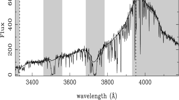
Figure 3.— An example QSO spectrum (Q0049-283). Vertical dotted lines are drawn at the emission wavelength of Ly$\alpha$ (right) and Ly$\beta$ (left). We have also plotted the continuum fitted by our procedure (see text) with a fitting length $L_{\rm fit}=50$ Å. The shading denotes regions excluded from the analysis. These are the regions blueward of Ly$\beta$, redward of Ly$\alpha$, within $50$ Å of either of the two DLA systems, and within $20$ Å of the QSO.

Third, we attempt to mitigate the effects of evolution over the redshift range subtended by each individual sample. The most noticeable effect of $z$ evolution is the decrease in the mean optical depth, which takes place as the Universe expands and the space density of hydrogen atoms decreases. In an Einstein-de Sitter Universe, the optical depth of photoionized gas evolves as $\tau\propto(1+z)^{4.5}$ owing to this effect. We follow Rauch et al. (1997) and CWKH in rescaling the fluxes in the spectra using this relation to the value they would have at the mean redshift of each sample (which is reasonable since all models are approximately Einstein-de Sitter at these redshifts). The spatial scales will also change due to the expansion of the Universe. To first order, we can correct for this by scaling all pixels to the size they would have in ${\rm\;km\;s^{-1}}$ at the mean redshift of the sample. In practice, this results in a constant scaling factor relating pixel sizes in Å to ${\rm\;km\;s^{-1}}$. There will be additional, second order effects due to the change in $H$ over the redshift range, but these will be small, and model dependent, so we do not attempt to correct for them.

Once we have treated the data as detailed above, we are left with a number of disjoint spectrum segments, of various lengths, because of the varying wavelength coverage and because the spectra have been broken up by the exclusion of DLA systems. We discard all segments that are shorter than a certain length (we use $100$ Å), chosen to be at least a factor of 3 larger than the maximum scale on which we measure $P(k)$, so that the effects of convolution with the Fourier transform of the window function are negligible. The data preparation procedure is illustrated in Figure 3, which shows the continuum fit and excluded wavelength regions for one of the spectra in the primary data sample.

3. Recovery of the power spectrum

The method we use for recovery of $P(k)$ from QSO Ly$\alpha$ forest spectra is described and tested in detail in CWKH. For completeness, we now give a brief account of the three principal steps in the procedure:

(1) We convert the spectra to one-dimensional linear density fields, by mapping the flux values in pixels monotonically to give them a Gaussian probability distribution function (PDF) with arbitrary normalization. This “Gaussianization” procedure is motivated by the fact that gravitational instability approximately preserves the rank order of (smoothed) densities (Weinberg 1992), so that one way of recovering the initial density field is to monotonically map the final densities back to the initial PDF, here assumed to be Gaussian. As the transformation between flux and density given by the FGPA is also local and monotonic, mapping the PDF of the flux directly to a Gaussian yields an initial density field, to the extent that these approximations hold. We note, however, that our results for the shape of $P(k)$ are insensitive to the precise nature of the transformation applied to the observed flux. For example, it was found in CWKH that the power spectrum of the flux itself has the same shape as the linear $P(k)$. We have found by numerical experiments that any transformation of the density that suppresses the contribution of the high density regions (including Gaussianization, $F=e^{-A\rho^{\beta}}$, or even truncation at $\rho/\bar{\rho}=5$) tends to produce a field whose power spectrum has the linear $P(k)$ shape. Thus, Gaussianization is not indispensable to the $P(k)$ recovery method, although it appears to be a useful way of “regularizing” spectra and thus reducing noise in the recovery (CWKH). In Section 5.4, we will briefly compare the shape of the primordial $P(k)$ to the non-linear $P(k)$ of the mass in simulations.

(2) We measure $P_{\rm 1D}(k)$, the one-dimensional power spectrum of this density field, using a Fast Fourier Transform. We convert this $P_{\rm 1D}(k)$ to the three-dimensional $P(k)$ by differentiation (Kaiser & Peacock 1991; CWKH),

$$P(k)=-\frac{2\pi}{k}\frac{d}{dk}P_{\rm 1D}(k).$$ (3)

Equation (3) assumes that the distribution of matter is isotropic with respect to the line of sight. Redshift-space distortions caused by peculiar velocities mean that this is not strictly true (Kaiser 1987), and these distortions must be taken into account for a truly accurate inversion of one-dimensional clustering (Hui 1998). We find in simulation tests (e.g., those in CWKH) that any error in the shape of the 3D $P(k)$ caused by redshift-space distortions is small and well within the statistical errors for the present observational determination of $P(k)$, although it could have a noticeable effect in some future samples. In step (3) below, we use our measured $P(k)$ shape as an input to the normalizing simulations. The $P(k)$ that we use for this purpose corresponds to $P(k)$ from equation (3) multiplied by $\exp(k^{2}r_{s}^{2}/2)$, with $r_{s}=34{\rm\;km\;s^{-1}}$, in order to compensate for power lost on small scales due to the finite resolution of the observations, as discussed in Section 2. However, we will only compare our recovered $P(k)$ to theoretical predictions on scales where $k<0.5/r_{s}$. In CWKH it was shown that the recovered $P(k)$ on these larger scales is insensitive to the details of the power restoration on smaller scales.

(3) The $P(k)$ resulting from step (2) is still of arbitrary amplitude. To determine the normalization, we use simulations that have Gaussian initial conditions (i.e., random Fourier phases) and an initial power spectrum with the same shape as our measured $P(k)$ (with small scale power restored as explained above) but with various linear theory amplitudes. The higher the power spectrum amplitude, the larger the fluctuations in the evolved mass density field, and hence the larger the predicted fluctuations in the observed flux. We can therefore pick the correct $P(k)$ amplitude by comparing clustering in spectra extracted from these simulations with the observations themselves. The statistic that we choose to make the comparison with is the three-dimensional power spectrum of the flux (more precisely, the power spectrum of $F/\langle F\rangle-1$, where $F$ is the ratio of the observed flux to the unabsorbed continuum). To distinguish this from $P(k)$ of the mass in plots, we will plot

$$\Delta^{2}_{\rm F}(k)=k^{3}P_{F}(k),$$ (4)

where $P_{F}(k)$ is the three-dimensional power spectrum of flux. The quantity $\Delta^{2}_{\rm F}(k)/2\pi^{2}$ is the contribution to the variance of the flux from an interval $d\ln k=1$. We run the simulations using the PM approximation, where we use a standard PM N-body code to evolve the mass distribution and assume (a) that the gas pressure effects in the low and moderate density regions are unimportant, so that the gas traces the dark matter, and (b) that the gas follows the power law temperature-density relation discussed in Section 1. The CWKH tests show that the PM approximation gives accurate predictions of the flux power spectrum relative to full hydrodynamic simulations. In making the artificial spectra from the normalizing simulations, there is one free parameter, in addition to the $P(k)$ amplitude, that can also influence the amplitude of flux fluctuations: the parameter $A$ of equation (2). Although it depends on physical quantities that are not known individually (such as $\Omega_{b}$, $\Gamma$, and $T_{0}$), $A$ as a whole can be set by appealing to one observational measurement that we have not yet used, the mean flux level in the spectra. We therefore fix $A$ in our normalizing simulations by picking the value for which the spectra have the same mean flux level as the observational measurements of Press, Rybicki & Schneider (1993, hereafter PRS). The mean flux level, $\langle F\rangle$, is often expressed in terms of an effective optical depth, $\overline{\tau}_{\rm eff}=-\ln{\langle F\rangle}$. Any uncertainty in the value of $\overline{\tau}_{\rm eff}$, and hence in $A$, is directly linked to uncertainty in the amplitude of $P(k)$. Our choice of a particular observational determination of this quantity could therefore affect our results appreciably. We will discuss this issue further later in the paper.

Given that the above procedure seems rather complicated, one could ask why we do not simply attempt a direct inversion of the flux to a mass distribution, using the FGPA as a guide, along the lines of the procedure proposed recently by Nusser & Haehnelt (1998). For purposes of determining the primordial $P(k)$, our more indirect procedure is more robust and more broadly applicable, for several reasons. First, our approach is relatively insensitive to what is occurring in saturated regions, which cannot be inverted directly from observations of Ly$\alpha$ absorption alone, and which in any case are less likely to obey the FGPA. Second, our method relies mainly on large scale clustering information; it therefore does not require data that fully resolve all Ly$\alpha$ features. Finally, the use of simulations in the normalizing procedure provides a convenient way to estimate the unknown parameter $A$, and it automatically includes the effects of non-linear gravitational evolution and peculiar velocities.

In our method of deriving $P(k)$, the assumption that primordial fluctuations are Gaussian enters mainly into the normalization step (3), since we use Gaussian fluctuations to initialize our normalizing simulations. If we adopted non-Gaussian initial conditions with the same $P(k)$ shape, then the $P(k)$ amplitude required in order to match the observed flux power spectrum with the observed $\overline{\tau}_{\rm eff}$ as a constraint might be different. The Gaussian assumption also motivates the Gaussianization procedure applied in step (1), but since the derived shape of $P(k)$ would be similar even without Gaussianization, it seems likely that recovery of the shape of $P(k)$ does not depend much on the assumption of Gaussian initial conditions. However, all of the tests in CWKH and in this paper are for initially Gaussian models, and the success of our method in recovering the shape and amplitude of $P(k)$ in non-Gaussian models would need to be tested on a case-by-case basis.

3.1. The shape of $P(k)$

Figure 4.— (a) $P(k)$ for the Gaussianized flux. The solid line is measured from the spectral regions between $z=2$ and $z=3$ (the fiducial sample). The dots were made by dividing the full sample into ten separate pieces and calculating $P(k)$ individually for each one. Open circles are plotted at the modulus of negative data points. (b) The 3D flux power spectrum, $\Delta^{2}_{\rm F}(k)\equiv k^{3}P_{F}(k)$, for the same samples plotted in (a).

We now turn to the analysis of the observational data. First, we measure the shape of $P(k)$ as described in steps (1) and (2) above, and also measure $\Delta^{2}_{\rm F}(k)$. In order to estimate errors, we take the whole data set [sample (2) of Section 2.1] and split it into 10 subsamples, of roughly equal length. We estimate $P(k)$ and $\Delta^{2}_{\rm F}(k)$ individually for each of the subsamples; the results are plotted as points in Figure 4. When Gaussianizing the flux to yield an initial density field, we set the $\sigma$ of the Gaussian PDF to be the same for each of the subsamples. For several of the subsamples, the values of $P(k)$ and $\Delta^{2}_{\rm F}(k)$ for the largest scale plotted in Figure 4a are unphysically negative, as are a few measurements on smaller scales. This can occur when the measured one-dimensional power spectrum is noisy, as the noise may result in regions with a positive slope, $\frac{d}{dk}P_{\rm 1D}(k)$, so that the inversion of equation (3) yields negative values for $P(k)$. The largest scale point plotted marks the limit where cosmic variance noise is small enough for this sample to allow us to make a reasonable inversion from one-dimensional to three-dimensional clustering. We will see later that the real maximum scale on which we can believe the $P(k)$ measurement appears to be slightly smaller, and is set by continuum fitting.

The solid lines in Figure 4 are the $P(k)$ and $\Delta^{2}_{\rm F}(k)$ measurements from the fiducial sample [sample (1) of Section 2.1], on which we will base most of our analysis. We will assign error bars to these measurements that are derived from the fractional error in the mean of the measurements from the 10 subsamples of the full data set described above. We base our error estimate on the variance among subsamples of the full data set rather than the smaller, $z$-limited, fiducial data set for two reasons: the inversion from 1D to 3D clustering is more manageable with the larger subsamples, and the errors based on a data set with a larger range in $z$ should be conservative, as there will be extra variance introduced by the larger $z$ evolution. We therefore assign fractional errors from the full sample to other samples, allowing for the difference in the number of independent data elements in each sample by scaling the fractional errors by the ratio of the square roots of the sample lengths.

We can see from Figure 4 that there is significant variation between the results for the different subsamples. Each subsample corresponds to roughly the length of one full Ly$\alpha$ to Ly$\beta$ region in a spectrum. The errors increase towards large scales because we are averaging over fewer independent modes. On small scales, we see a turnover, due to the finite observational resolution of our data sample. The lowest resolution data that forms part of our sample has a FWHM resolution of 2.3 Å. As discussed in Section 2, this is similar to the smallest scale for which the simulation tests of CWKH verified that the linear $P(k)$ can be correctly recovered. Because of this limitation, we should only regard our results on scales larger than $k\sim 0.02({\rm km\;s}^{-1})^{-1}$ as being representative of the true shape of $P(k)$.

Figure 5.— Tests of the effect of changing the length over which the continuum is fitted, $L_{\rm fit}$. See Section 2.2 for details of the fitting procedure. (a) The Gaussianized $P(k)$. (b) The 3D flux power spectrum, $\Delta^{2}_{\rm F}(k)$. Error bars are derived from the error on the mean taken from splitting the sample into 10 subsamples.

The data preparation procedure described in Section 2.2 involves several operational parameters, the choice of which could conceivably affect our results. One of these is the length $L_{\rm fit}$ over which the continuum is fitted. In Figure 5 we test the effect of using different values of $L_{\rm fit}$. Again we plot both $P(k)$ and $\Delta^{2}_{\rm F}(k)$, this time for the fiducial sample. The error bars have been determined in the manner explained previously.

The smallest $L_{\rm fit}$ we try, $25$ Å, is obviously too small, being similar in size to the largest wavelength on which we measure $P(k)$. We try this value as an experiment, to see how this poor choice of $L_{\rm fit}$ will affect our measurements. By comparing panels (a) and (b) of Figure 5, we can see that the effects are different for $P(k)$ and for $\Delta^{2}_{\rm F}(k)$. On scales $k<4\times 10^{-3}({\rm\;km\;s^{-1}})^{-1}$ and larger, the continuum fitting has completely eliminated power in $P(k)$, but $\Delta^{2}_{\rm F}(k)$ has increased. This difference may reflect the fact that the Gaussianized field used to measure $P(k)$ has more prominent low density regions, as the Gaussianization stretches out the PDF of low densities into a Gaussian tail. These low density regions, being closer to the continuum, may be more influenced by fitting. When we use more reasonable values for $L_{\rm fit}$, including our fiducial value of $50$ Å, we can see that the two largest scale points are affected by the choice of fitting length, and for $k<2\times 10^{-3}({\rm km\;s}^{-1})^{-1}$ the systematic variation is outside the statistical errors. We will therefore discard the largest scale point when making use of our results. It is interesting that increasing $L_{\rm fit}$ appears to yield less power, although it is not certain whether this represents a trend or merely a statistical fluctuation.

One might worry that with our relatively low spectral resolution we will fit the continuum systematically low everywhere. One way of checking to see if this is a problem is to change the clipping level below which points are discarded during the fitting process. The usual value is $2\sigma$ (where $\sigma$ is the error on the flux at a point), but if we change it to $1\sigma$ we tend to fit the continuum much higher, almost certainly too high. The mean effective optical depth of the sample, $\overline{\tau}_{\rm eff}$, increases by $25\%$ to 0.30, but this change has no direct impact because we use the PRS measurement of $\overline{\tau}_{\rm eff}$ to fix the value of $A$, not the value from the sample itself. What is important is that $P(k)$ and $\Delta^{2}_{\rm F}(k)$ hardly change at all, as shown by the open squares in Figure 5. We have also tried raising the continuum uniformly everywhere by $10\%$, and we again find that this has a negligible effect on our results.

As we will see by considering other potential factors, the continuum fitting process appears to act as a limit to the largest scales on which we can measure $P(k)$ from the current data set. It may be that data with higher spectral resolution would allow more accurate continuum fitting and hence enable measurement of $P(k)$ at larger scales. In future work we plan to carry out a systematic analysis of continuum fitting procedures using larger volume simulations (for which the true continuum is known). Such analysis might suggest better ways of determining the continuum, perhaps involving a totally different technique (see, e.g., PRS), and it would help us understand the interplay of spectral resolution, signal-to-noise ratio, and continuum fitting in limiting the accuracy and dynamic range of $P(k)$ recovery. Continuum fitting also has an important impact on other statistical measurements of the Ly$\alpha$ forest, such as $\overline{\tau}_{\rm eff}$ and the flux decrement distribution function (Rauch et al. (1997)). Although a detailed investigation of these issues is beyond the scope of this paper, we can already surmise from consideration of Figure 5 that our $P(k)$ measurement is likely to be reliable out to a wavelength $\lambda\sim 2300{\rm\;km\;s^{-1}}$, which for $\Omega_{0}=1$ corresponds to a comoving scale $\sim 12\;h^{-1}{\rm Mpc}$. On scales smaller than this, reasonable variations in the continuum fitting procedure have no significant influence on our derived $P(k)$.

Figure 6.— Tests of the data preparation procedure. The points labeled “fiducial” are for $z=2$ to $z=3$ and have the continuum fitted over a 50Å region, have $(1+z)^{4.5}$ scaling of $\tau$, a 20 Å proximity gap, and a 100 Å region excluded around DLA systems. The other points show the effect of varying these parameters. (a) The Gaussianized $P(k)$. (b) The 3D flux power spectrum, $\Delta^{2}_{\rm F}(k)$.

In Figure 6 we vary the other parameters used in the data preparation of Section 2.2 and compare with results for the fiducial parameter choices. We can see that changes such as not scaling the optical depths to the mean redshift, or increasing the QSO proximity gap to $100$ Å from the fiducial value of $20$ Å, cause only minor changes to $P(k)$, within the $1\sigma$ errors. Even keeping the DLA systems as part of the analyzed portion of the spectra, obviously not a reasonable thing to do, does not change the results by much; there is a small change in $P(k)$ and $\Delta^{2}_{\rm F}(k)$ near $k\sim 0.05({\rm\;km\;s^{-1}})^{-1}$, which is probably the signature of power on the scale of the DLA systems themselves. These tests therefore increase our confidence in the robustness of the measurements of $P(k)$ and $\Delta^{2}_{\rm F}(k)$. For larger, future samples, different treatments of the data may yield systematic differences of results that rival the statistical errors. This does not appear to be the case here, indicating that the procedures we have adopted are adequate for our current data and objectives.

3.2. The normalization of $P(k)$

As outlined previously, we use simulations to normalize our estimate of $P(k)$. The $P(k)$ we use as an input to the normalizing simulations is slightly different from the measured $P(k)$ plotted in Figures 5 and 6, in that we restore small scale power that was suppressed by the limited observational resolution. In CWKH, it was shown that missing power on small scales only has a small effect on $\Delta^{2}_{\rm F}(k)$ at the large scales we use for normalization (see Figure 9 of CWKH). We therefore do not need to make this correction for lost small scale power very precisely. As described at the beginning of Section 3, we “unsmooth” $P(k)$ using a Gaussian filter, so that

$$P_{S}(k)=P(k)\times e^{k^{2}r_{s}^{2}/2},$$ (5)

where $r_{s}=34{\rm\;km\;s^{-1}}$ and $P_{S}(k)$ is the power spectrum used in the normalizing simulations. We also extrapolate $P(k)$ above the largest measured point using an $n=-1$ power law.

The PM simulations have $128^{3}$ particles on a $256^{3}$ grid in a periodic box $4170{\rm\;km\;s^{-1}}$ on a side. We assume $\Omega_{0}=1$ and $\Lambda_{0}=0$ (and $H_{0}=50{\rm\;km\;s^{-1}}\;{\rm Mpc}^{-1}$) when running the simulations, so that the box size is $22.22\;h^{-1}{\rm Mpc}$ comoving. CWKH have shown that the choice of cosmological parameters has a negligible effect on the results provided that one works in the observed ${\rm\;km\;s^{-1}}$ units. We choose $\Omega_{0}=1$ for the simplifying reason that we can use different outputs of a single simulation to represent different mass fluctuation amplitudes, since $\Omega=1$ at all redshifts and the linear theory fluctuation amplitude is proportional to the expansion factor, $a(t)$. The initial density field is set up using $P_{S}(k)$ and Gaussian random phases. We average results from 4 different realizations that use different random seeds. The simulations are run so that the expansion factor, $a$, increases by a factor of 16.8 from the initial conditions to the most evolved output, in 84 equal steps of $\Delta a=0.2$.

Figure 7.— The 3D power spectrum of the flux for the fiducial sample, compared to outputs from normalizing simulations that use $128^{3}$ particles in a $22.22\;h^{-1}{\rm Mpc}$ box ($\Omega_{0}=1$). The different curves are labeled by the expansion factor at each simulation output, normalized so that $a=1$ corresponds to the amplitude determined to best fit the observational results. Only the solid points are used to fix the normalization. The open points on smaller scales are affected by the finite resolution of the spectra and the simulations, and largest scale point is systematically uncertain because of continuum fitting (Section 3.1).

We extract spectra from the simulations, for several different output times, using the methods described in CWKH. We use a temperature-density relation of the form given by equation (1), with $T_{0}=5600$K and $\alpha=0.6$. We adjust the mean effective optical depth $\overline{\tau}_{\rm eff}$ (by varying $\Omega_{b}^{2}/\Gamma$) so that $\overline{\tau}_{\rm eff}=0.28$, the PRS value at $z=2.5$. We extract 2000 spectra in total at each output time and calculate $\Delta^{2}_{\rm F}(k)$ from them. The results are plotted in Figure 7, where the curves for different output times are labeled with the expansion factor $a$, and $a=1$ has been chosen to correspond to the normalization appropriate for the observational results (which we shall describe below). From Figure 7, we can see that changing the underlying amplitude of mass fluctuations results in a clear change in $\Delta^{2}_{\rm F}(k)$ (recall that $\overline{\tau}_{\rm eff}$ is the same for all spectra). We will restrict our quantitative use of the data to large scales, with $k<0.02({\rm km\;s}^{-1})^{-1}$, which in practice means using the 2nd through the 8th observational points (we discard the first point because of continuum fitting uncertainties). On smaller scales we do not know the initial $P(k)$ accurately, and the predicted $\Delta^{2}_{\rm F}(k)$ depends on physical assumptions and the resolution of the simulations.

To determine the normalization of $P(k)$, we must decide which of the $\Delta^{2}_{\rm F}(k)$ curves in Figure 7 (or interpolation between these curves) is closest to the observational results. One possible method for determining the correct normalization involves a maximum likelihood fit of the simulation results to the observational data, where we seek to maximize the likelihood by minimizing

$$\chi^{2}=\sum_{ij}[\Delta^{2}_{F}(k_{i})-\Delta^{2}_{Fsim}(k_{i},a)]C^{-1}_{ij}[\Delta^{2}_{F}(k_{j})-\Delta^{2}_{Fsim}(k_{j},a)].$$ (6)

Here $\Delta^{2}_{F}(k_{i})$ is the observed value of $\Delta^{2}_{\rm F}(k)$ at $k=k_{i}$ and $\Delta^{2}_{Fsim}(k_{i},a)$ is the equivalent quantity measured from simulation outputs at expansion factor $a$. The covariance matrix of the data points, $C$, is estimated using the observational data split into subsamples. If we use this procedure, we obtain a normalization of $P(k)$ with errors of $(+10\%,-9.5\%)$. We have also applied this procedure using a jackknife estimator to determine $C$ from the ten subsamples, with very similar results.

Despite its statistical logic, we have decided not to adopt the maximum likelihood determination of the normalization and error but instead to rely on a simpler estimator. There are two main reasons for this. First, we find that the above procedure yields an unrealistically low value of $\chi^{2}$ for the best fitting output. The low $\chi^{2}$ arises because the $P(k)$ used in the simulations is measured from the observational data themselves, so that the shape of $\Delta^{2}_{\rm F}(k)$ in the simulations is more correlated with the observations than the cosmic variance error bars suggest. Second, and probably more important, the points on small scales, with small statistical errors, are weighted most highly in the maximum likelihood fit. These points are also those most likely to be affected by systematic errors in the simulations resulting from resolution effects (see below) or uncertainty in the input physical assumptions (see CWKH). We therefore adopt an estimator that depends more evenly on the data points and that condenses the information about the amplitude of $P(k)$ into one number,

$$S=\sum_{i}\Delta_{F}^{2}(k_{i}).$$ (7)

The sum is over the 2nd to the 8th data points, as explained above. Because the variance of the flux is $\int_{0}^{\infty}\Delta_{F}^{2}(k)d{\rm ln}k/2\pi^{2}$ and our data points are evenly spaced in ${\rm ln}k$, the quantity $S$ is simply the contribution to the flux variance from the wavenumber range over which we estimate the power spectrum. Although this estimator does not weight the data optimally in a strictly statistical sense, it is less sensitive to systematic errors on small scales, and by using it we arrive at a conservative estimate of the $P(k)$ normalization error.

The observed value of $S$ is our diagnostic for the amplitude of $P(k)$ — the higher the amplitude, the larger the value of $S$ predicted by the normalizing simulations. We choose the best fit amplitude to be the one for which the predicted $S$ matches the observed value (using linear interpolation between the two closest simulation outputs). We obtain the $1\sigma$ uncertainty by measuring $S$ separately for each of the 10 subsamples of the full data set [sample (2) in Section 2.2], converting the $1\sigma$ error on the mean of $S$ into a corresponding uncertainty in the mass fluctuation amplitude. Since the relationship between $S$ and the amplitude is fairly linear, we would get similar results if we instead determined the amplitude separately for each subsample and took the $1\sigma$ error on the mean amplitude. Normalization errors for subsets of the data, such as the fiducial sample and the other samples of Section 2.2, come from scaling the errors on $S$ by the ratio of the square roots of the lengths of the spectra involved, as was done with the errors on the individual $P(k)$ points.

After applying this procedure, we find the $\pm 1\sigma$ uncertainty on the normalization of the fiducial ($z=2-3$) sample to be $(+17.0\%,-16.5\%)$ in the fluctuation amplitude $a$. The normalization itself is $15\%$ higher in $a$ than that which results from applying the maximum likelihood fit of equation (7).

Figure 8.— The effect of varying $\overline{\tau}_{\rm eff}$ in the normalizing simulations. The dashed lines show the $1\sigma$ errors on the value of $\overline{\tau}_{\rm eff}$ from PRS and how they correspond to an uncertainty in $a$. The errors are $\sim\pm 4\%$ on $\overline{\tau}_{\rm eff}$ and ($+12\%,-9\%$) on $a$.

An important additional source of error is uncertainty in the value of $\overline{\tau}_{\rm eff}$. The value we use is given by the PRS formula $\overline{\tau}_{\rm eff}=0.0037(1+z)^{3.46}$. PRS measured their result from a sample of 29 low resolution QSO spectra. They estimated the continuum in the Ly$\alpha$ forest region by extrapolating the continuum observed on the red side of the Ly$\alpha$ emission line. The results are consistent with those measured from high resolution Keck spectra (Rauch et al. 1997) using a polynomial continuum fitting technique blueward of Ly$\alpha$. The smaller Keck sample has larger statistical errors, but its consistency with the PRS result makes us reasonably confident that the value of $\overline{\tau}_{\rm eff}$ we use is close to the true one. However, we note that discrepant, lower results for $\overline{\tau}_{\rm eff}$ have been published by other authors (e.g., Zuo & Lu (1993); Dobrzycki & Bechtold (1996)), and the issue is not settled.

We quantify the influence of $\overline{\tau}_{\rm eff}$ on the $P(k)$ amplitude by making new spectra from our normalizing simulations, with different values of $\overline{\tau}_{\rm eff}$. We then carry out our normalizing procedure using the weighted sum of equation (7) to find the best fitting value of $a$ for the observations using the new spectra. The results are shown in Figure 8. Increasing $\overline{\tau}_{\rm eff}$ for a given amplitude of mass fluctuations increases the fluctuations in $\Delta^{2}_{\rm F}(k)$, since it requires us to choose a larger value of $A$ in equation (2). As a result, we find a lower value for $a$. The $1\sigma$ error that PRS give on their $\overline{\tau}_{\rm eff}$ measurement corresponds to $4\%$ at $z=2.5$. This can be translated directly to an error in $a$ of ($+12\%,-9\%$), as shown in Figure 7.

In order to combine these two contributions to the normalization uncertainty, we first calculate the likelihood distribution for the amplitude of mass fluctuations for each of the sources of error taken individually, assuming that the errors on $\overline{\tau}_{\rm eff}$ and on the weighted sum $S$ of equation (7) are each Gaussian distributed. We then convolve the likelihood distributions and find the total uncertainty, which is $(+20\%,-17\%)$ in the amplitude of mass fluctuations and $(+45\%,-31\%)$ in $P(k)$. The combination of errors is described in more detail in Section 5.1.

The $\overline{\tau}_{\rm eff}$ error is smaller than the main source of error, but it is nonetheless important. It would be worth investigating the measurement of $\overline{\tau}_{\rm eff}$ in detail, as a more accurate measurement is critical to obtaining more accurate determinations of $P(k)$ using larger samples of QSO data. As $\overline{\tau}_{\rm eff}$ in our approach sets the value of the parameter $A$ in equation (2), it determines how well we can measure the level of “bias” between $\tau$ and the mass fluctuations. Measurements of $\overline{\tau}_{\rm eff}$ are also crucial for constraining the parameters that are subsumed into $A$, such as $\Omega_{b}$ (see Rauch et al. 1997; Weinberg et al. 1997b).

Although we do not use $\Delta^{2}_{\rm F}(k)$ information on small scales in our normalization of $P(k)$, we might also expect the resolution of the simulations to have some effect on $\Delta^{2}_{\rm F}(k)$ on large scales. For example, if the normalizing simulations are of insufficient resolution, small scale fluctuations that should be near saturation, or at least away from the linear part of the curve of growth, might instead be smoothed out, and therefore contribute more to $\overline{\tau}_{\rm eff}$. The interplay between $\overline{\tau}_{\rm eff}$ and the amplitude of mass fluctuations described above would then lead to a systematic offset in the normalization. To check that our normalizing simulations have sufficient resolution, we have run some simulations with higher resolution and some with lower resolution. Figure 9a shows results for the low resolution runs, which use the same phases and box size as the original simulations, but have only $64^{3}$ particles instead of $128^{3}$. The mean interparticle separation, listed on the plot legend, is therefore a factor of two larger. For two of the plotted output times, this lowering of resolution has increased $\Delta^{2}_{\rm F}(k)$ systematically on large scales. Normalizing $P(k)$ using these low resolution simulations would result in a mass fluctuation amplitude $\sim 20\%$ lower. The effect on $\Delta^{2}_{\rm F}(k)$ at smaller scales, $k>0.015({\rm km\;s}^{-1})^{-1}$, is much stronger, since this is the regime where the lowered resolution comes directly into play, but these scales do not enter into our normalization procedure.

Figure 9.— The effect of varying resolution in the normalizing simulations. We plot the power spectrum of the flux for a few different output times. (a) $4170{\rm\;km\;s^{-1}}$ ($22.22\;h^{-1}{\rm Mpc}$ for $\Omega_{0}=1$) box simulations, with the same phases, but with different mean interparticle separations $d_{p}$. The results shown in this panel are an average of 4 realizations for each resolution. (b) Results from two single simulations (same phases) in a $2085{\rm\;km\;s^{-1}}$ ($11.111\;h^{-1}{\rm Mpc}$ for $\Omega_{0}=1$) box with different interparticle separations.

Figure 9b compares results at our standard resolution to results at higher resolution. Here we have only run one realization for each of the two resolutions, with identical phases, in a box of side length $11.11\;h^{-1}{\rm Mpc}$. As the phases are different from the panel (a) runs, and the cosmic variance errors are large (the volume of space simulated is $1/32$ of that in panel [a]), we cannot compare panels (a) and (b) directly. We can compare the dotted curves, which have the same resolution as the original simulations, to the solid curves, which show the effect of increasing the spatial resolution by a factor of two. This time there is no systematic offset between the two, so it appears that our original simulations have sufficient resolution. The standard normalizing simulations have the same mass resolution as the SPH simulations analyzed in CWKH (but lower gravitational force resolution), and each has eight times the volume. There is a systematic difference between the standard and high resolution simulations of Figure 9b at high $k$, suggesting that the depression of the small scale $P(k)$ found in the CWKH tests is caused at least in part by the finite mass resolution of the SPH simulations.

4. The effect of fluctuations in the ionizing background

Before examining and discussing our $P(k)$ results in more detail, we investigate another potential source of systematic error, clustering in the flux caused by fluctuations in the ionizing background. If the ionizing background is not uniform, as we have assumed, but instead exhibits substantial inhomogeneities, then fluctuations in $\tau$ will be caused by fluctuations in the spatially varying value of $\Gamma$ in equation (2), as well as by fluctuations in the mass density. The UV background (UVBG) is produced mainly by discrete sources, such as QSOs and starburst galaxies. Whether this discreteness has an important effect on our $P(k)$ determination depends on the scale and amplitude of the clustering induced by the non-uniformity of the UVBG compared to that produced by intrinsic clustering in the mass. By claiming that we are able to measure $P(k)$ for the mass, we are effectively assuming that the UVBG is uniform on the scales $<10\;h^{-1}{\rm Mpc}$ that we can access with our current observational data.

Previous work on this issue has examined the effect of UVBG fluctuations on randomly distributed Ly$\alpha$ clouds (Zuo 1992; Fardal & Shull 1993). In this paper we simulate the fluctuations caused in uniformly distributed gas, using the FGPA, and also the effect of modulating observed QSO spectra with additional UVBG fluctuations derived from simulations. The case for which we expect there to be the largest fluctuations is a UVBG entirely generated by QSOs, which have a very low space density. We will therefore deal with this case first and in most detail.

Our UVBG simulations are set up in a universe with $H_{0}=50{\rm\;km\;s^{-1}}\;{\rm Mpc}^{-1}$, $\Omega_{0}=0.2$, and $\Lambda_{0}=0$, and a box of size 370 proper Mpc at $z=2.5$ (which corresponds to $79310{\rm\;km\;s^{-1}}$). We populate this box with QSOs, using luminosities drawn from the luminosity function of Haardt & Madau (1996), with a lower cutoff at $M_{B}=-23$. We try simulating both Poisson distributed and clustered QSO distributions. The clustered QSO positions are chosen by first generating a Gaussian linear density field in the box using a power spectrum appropriate for a $H_{0}=50{\rm\;km\;s^{-1}}\;{\rm Mpc}^{-1}$, $\Omega_{0}=0.2$ CDM model (taken from Efstathiou, Bond, & White 1992). We select all regions in this field that have a density above a certain threshold and populate them randomly with QSOs. As shown by Kaiser (1984), thresholding produces a distribution of QSOs that are clustered more strongly than the underlying mass. We choose the threshold height so that the scale at which the autocorrelation function of the QSOs is unity is $r_{0}=10\;h^{-1}{\rm Mpc}$ (comoving).

The factor that most strongly influences the level of UVBG fluctuations is the attenuation length of the QSO flux. At high redshifts, the intergalactic medium has a substantial optical depth to ionizing photons. Fardal & Shull (1993) recommend parameterizing the attenuation of ionizing radiation by intergalactic gas with an attenuation length, $r_{\rm att}$, defined so that radiation reaching a distance $r$ from a source is attenuated on average by a factor $e^{-(r/r_{\rm att})}$. Fardal & Shull (1993) and Haardt & Madau (1996) estimate that $r_{\rm att}\simeq 100$ proper Mpc (for $h=0.5$) at $z=2.5$. The attenuation length rises rapidly with increasing redshift, as the Universe becomes more optically thick. We will try using both $r_{\rm att}=100$ Mpc and $r_{\rm att}=50$ Mpc in our simulations.

To generate spectra from our UVBG simulations, we randomly select lines of sight through the box and calculate the intensity of UV radiation at each point along them, summing the contributions of all the QSOs in the box. We assume Euclidean space, which should be a good approximation at high redshift, and periodic boundary conditions. We therefore apply an inverse-square law to the radiation, which is additionally attenuated according to the attenuation law described above. Because of the finite box size, we cut off the flux after it has traveled one full box side length. The optical depth at each point in the spectra is calculated according to equation (2), with $\rho_{b}(x)=1$ (the cosmic mean) and $\Gamma(x)\propto J(x)$, where $J(x)$ is the UV radiation intensity at point $x$. The value of $A$ is set so that $\overline{\tau}_{\rm eff}$ for the spectra is equal to the PRS value of 0.28.

Figure 10.— Top five panels: Lines of sight through a universe with $h=0.5,\Omega_{0}=0.2,\Lambda=0$, in which a uniform IGM is photoionized by a discrete population of QSOs drawn from the Haardt & Madau (1996) luminosity function. The lines represent the transmitted flux assuming the PRS value of $\overline{\tau}_{\rm eff}$, clustered QSOs, and a 50 Mpc attenuation length, $r_{\rm att}$. The full simulation occupies a 370 proper Mpc box, which is 79310 km/s on a side at $z=2.5$. The bottom panel displays a portion of the spectrum of Q2206-199. The bar in the top panel is of length $3000{\rm\;km\;s^{-1}}$, the largest wavelength plotted in the previous $P(k)$ figures.

In Figure 10, we show portions of five sample UVBG simulation spectra (the simulation box is more than twice the length of the spectra shown), together with a piece of the spectrum of Q2206-199. The model spectra represent a universe in which the IGM is uniform density and absorption fluctuations are caused only by inhomogeneities of the UVBG. The fluctuations are mild and have a large coherence scale, very different from the observed spectrum shown in the bottom panel. The bar shown in the top panel is of length $3000{\rm\;km\;s^{-1}}$, corresponding to the largest wavelength for which we have tried to measure $P(k)$. The fluctuations caused by UVBG inhomogeneity are small compared to the observed flux variations on this scale (a point that we will demonstrate quantitatively below). It was shown in Section 3.1 that this scale is already larger than the minimum scale that is affected by continuum fitting. Looking at Figure 10, it seems as though UVBG fluctuations will therefore not limit our ability to measure $P(k)$ on these scales and below. We note that the assumptions employed in Figure 10 (strongly clustered QSOs and an attenuation length half the expected value) are those that tend to maximize the fluctuations.

Figure 11.— The 3D flux power spectrum for lines of sight through a uniform density medium with the PRS value of $\overline{\tau}_{\rm eff}$ and an inhomogeneous UVBG. We show results for clustered and Poisson distributed QSOs with two different values of the attenuation length.

We can examine the effect of UVBG fluctuations quantitatively by measuring $\Delta^{2}_{\rm F}(k)$ for the UVBG simulation spectra. The results are plotted in Figure 11, for Poisson distributed QSOs and clustered QSOs, and for the two different values of $r_{\rm att}$. Reducing the attenuation length by a factor of two has a significant effect, raising $\Delta^{2}_{\rm F}(k)$ by roughly a factor of two, while the change induced by clustering the QSOs is barely measurable. The value of $\Delta^{2}_{\rm F}(k)$ in the UVBG simulations is $5\%$ or less of $\Delta^{2}_{\rm F}(k)$ in the observations for the largest scale plotted, and $\sim 1\%$ for the largest scale reliable enough to use in our analyses, $k=2.7\times 10^{-3}({\rm km\;s}^{-1})^{-1}$. On very large scales ($\lambda\sim 100-200\;h^{-1}{\rm Mpc}$ for $\Omega=1$), the UVBG fluctuations should become important, but these scales are beyond the range of the techniques we are using here. The results of our analysis agree with the conclusions reached by Fardal & Shull (1993), that the UVBG fluctuations have a relatively small amplitude and a large coherence scale. We should bear in mind that at higher redshifts, if QSOs are the dominant source of UVBG radiation, then the fluctuations should increase, perhaps to a detectable level, because of the observed decrease in the space density of QSOs past $z=3$ (Warren et al. 1994) and because of the decreasing transparency of the IGM.

Figure 12.— The 3D power spectrum of the observed QSO spectra modulated by the inhomogeneous UV background taken from the UVBG simulations used in Figure 10 (clustered QSOs, $r_{\rm att}=50$ Mpc). The error bars represent the variance measured from modulating the observations ten times using different realizations of the simulated UVBG. The lines represent our fiducial result (see previous figures).

We can look at the effects of inhomogeneity in the UVBG in a different way by modulating observed QSO spectra with additional fluctuations derived from our UVBG simulations. This should give us an idea of what occurs when density fluctuations and UVBG fluctuations are taken together. We have done this by taking values of $J$ along lines of sight in the UVBG simulations and multiplying $\tau$ in the observations by $\overline{J}/J(x)$, where $\overline{J}$ is the mean radiation intensity. The results are plotted in Figure 12, with error bars representing the variance of the results for 10 separate realizations of the UVBG. There are only very small changes with respect to the unmodulated results. The variance between realizations is apparent, even on small scales. The effects of UVBG fluctuations on small scales are probably due to their manifestation as changes in the mean optical depth, which slightly increase the variance in the measured $P(k)$ from spectrum to spectrum.

Our UVBG simulations could be extended to include other potential characteristics of the QSO population. For example, it is possible that QSOs emit their Ly$\alpha$ radiation in a highly beamed way, or else that they have short lifetimes compared to the light travel time across $r_{\rm att}$. If either of these effects were operating, the effective space density of QSO sources responsible for the UVBG should be larger than that given by the luminosity function we have used. This increased space density would counterbalance any extra inhomogeneity in the radiation emitted by the sources themselves.

If the sources of radiation are more numerous than QSOs, we expect the UVBG to be more homogeneous. We can make a rough estimate of the size of fluctuations using the model of Fardal & Shull (1993, see also Kovner & Rees 1989). At a certain distance from a source, $r_{p}$, the UV intensity produced by the source is equal to that produced by the UVBG, so that $J_{S}(r_{p})=\overline{J}$. We define the effect of this local UV radiation to be strong if $r<r_{p}$. If all sources have the same luminosity, and a space density $\overline{n}$, then $r_{p}=(4\pi\overline{n}r_{\rm att})^{1/2}$. The volume filling factor, $f$, of regions where the effect of local UV radiation is strong is $4\pi r_{p}\overline{n}/3$. For small $f$, the variance of UVBG fluctuations is approximately equal to $f$. If the sources of UVBG radiation are starburst galaxies with mean separations of $5\;h^{-1}{\rm Mpc}$ comoving, then, using Fardal & Shull’s value for $r_{\rm att}$ at $z=2.5$, we find $f\sim 10^{-3}$ (if $\Omega_{0}=1$). This is extremely small, showing that the contribution to the UVBG of galaxies and other sources with the same or greater number density will be very smooth. This smoothness will be enhanced by re-emission of UVBG radiation from Ly$\alpha$ forest and Lyman limit systems, which are even more numerous. This smoothing effect was pointed out by Haardt & Madau (1996), who estimated that recombination radiation from these systems contributes about $30\%$ of the UVBG at $z=3$.

In this Section we have studied the possible effect of an inhomogeneous UVBG, something that has not previously been incorporated into simulations of the Ly$\alpha$ forest. Other physical processes such as quasar outflows or supernova shock heating of the IGM on the outskirts of galaxies could also affect the clustering seen in Ly$\alpha$ spectra, but most of these would be confined to high density regions with a small volume filling factor. They would therefore have little impact on the large scale mass clustering inferred from the Ly$\alpha$ forest, just as shock heating, collisional ionization, and star formation, processes that are included in SPH simulations but not in the PM approximation, have negligible impact on the recovery of $P(k)$ (see CWKH). A physical effect that could have an impact in low density regions is inhomogeneous heating of the IGM during helium reionization (Miralda-Escudé & Rees (1994)), which could produce spatial fluctuations in the temperature-density relation if helium reionization is sufficiently late and sufficiently patchy. However, if we consider equation (2) in the limit of weak fluctuations, we see that the fluctuations in temperature at fixed density would need to be more than twice as large as the fluctuations in density on the same spatial scale in order to have an equal effect, since $\tau\propto\rho_{b}^{1.6}T_{0}^{-0.7}$.

In the long run, rather than trying to investigate all possible sources of spurious clustering, we should look for support for the gravitational instability interpretation of Ly$\alpha$ forest fluctuations in the observational data themselves. Already many aspects of the observational Ly$\alpha$ forest data can be reproduced and explained by the scenario (see, e.g., Bi & Davidsen 1997; Rauch et al. 1997). One specific test of our approach is the measurement of the evolution of $P(k)$ with redshift. The $P(k)$ we measure should change in the way predicted by linear theory, keeping the same shape and increasing in amplitude in a way that (in detail) depends on $\Omega_{0}$ and $\Lambda_{0}$. It seems very unlikely that any non-gravitational processes could precisely mimic this behavior, so if linear growth were seen in the data it would provide strong evidence for the validity of the $P(k)$ measurement. Although the observational sample we are using in this paper is too small to carry out this test unambiguously, we are at least able to split the sample into two redshift halves and see if there are any gross deviations from linear growth. We will do this below.

5. Results

5.1. Tabulation of $P(k)$ and a power law fit

In Table 1, we give the values of $P(k)$ and their $1\sigma$ errors for the seven points where we believe that our measurement is representative of its primordial value. The $1\sigma$ errors were calculated in Section 3.1, from the scatter between results for 10 subsamples of the data. They primarily represent uncertainties in the shape of $P(k)$, as there is a separate normalization uncertainty that applies to all points equally. This normalization uncertainty was estimated in Section 3.2, again from the scatter in results between 10 subsamples of the data. The covariance matrix of the data values (calculated using the 10 subsamples) has some non-negligible off-diagonal terms, which quantitative evaluation of models should take into account.

Table 1 The linear $P(k)$ at $z=2.5$. We give the wavenumber $k$, $P(k)$, and the $1\sigma$ error on $P(k)$. An additional error should also be assigned to the normalization of all points, which is $+40\%,-29\%$ in $P(k)$ ($1\sigma$).

$k$ $({\rm km\;s}^{-1})^{-1}$	$P(k)$ $({\rm\;km\;s^{-1}})^{-3}$	$\sigma$[$P(k)$]
$2.66\times 10^{-3}$	$3.6\times 10^{8}$	$1.9\times 10^{8}$
$3.52\times 10^{-3}$	$1.7\times 10^{8}$	$8.9\times 10^{7}$
$4.65\times 10^{-3}$	$9.4\times 10^{7}$	$2.8\times 10^{7}$
$6.14\times 10^{-3}$	$3.4\times 10^{7}$	$1.0\times 10^{7}$
$8.12\times 10^{-3}$	$1.7\times 10^{7}$	$5.1\times 10^{6}$
$1.07\times 10^{-2}$	$1.3\times 10^{7}$	$3.8\times 10^{6}$
$1.42\times 10^{-2}$	$6.2\times 10^{6}$	$1.1\times 10^{6}$

As the estimated errors on our points are fairly large, and we cover a limited range in $k$, the information in our $P(k)$ measurement can be effectively summarized by the amplitude and slope of a power law fit to the data points. When determining the parameters of this fit, we can include the effect of covariances between data points, which are not given in the Table above. To eliminate as much as possible the covariance between the fit parameters themselves, we have chosen to describe the amplitude of the fit by the value of $P(k)$ at a pivot wavenumber $k_{p}$ near the center of the data range. The form we fit is therefore

$$P(k)=P_{p}\left(\frac{k}{k_{p}}\right)^{n}.$$ (8)

We perform a $\chi^{2}$ fit to the seven data points, including the full covariance matrix for the points [as in equation (6), though here it is the Gaussianized flux $P(k)$ rather than $\Delta^{2}_{\rm F}(k)$ that enters]. We try several values for the pivot wavenumber and choose $k_{p}=0.008({\rm km\;s}^{-1})^{-1}$, the value for which the covariance between $P_{p}$ and $n$ is minimized. In evaluating the covariance matrix of the $P(k)$ data points from the ten subsamples of the full data set, we find that the fluctuations of neighboring data points are usually anticorrelated, probably because of the differentiation involved in going from the 1D power spectrum to the 3D power spectrum (equation [3]). As a consequence, the statistical error on the power law slope $n$ is smaller than it would be if we ignored the covariances in our $\chi^{2}$ evaluation. Because the anticorrelated structure of the covariance matrix significantly influences the error estimate and the estimate of the covariance matrix from the data subsamples is itself noisy, we regard our estimate of the error on $n$ as itself significantly uncertain. If we ignored covariance terms when fitting $n$, we would get error bars $\sim 45\%$ larger ($n=-2.30\pm 0.26$) than those reported below based on using the full covariance matrix.

Figure 13 shows the best fit power law, together with the points from Table 1. Figure 14a shows contours of constant $\Delta\chi^{2}$ for the fit, where $\Delta\chi^{2}=\chi^{2}(P_{p},n)-\chi^{2}(P_{p\min},n_{\min})$ and $(P_{p\min},n_{\min})$ are the values of the fit parameters for which the $\chi^{2}$ is a minimum. The 1,2 and $3\sigma$ contours of joint confidence in the fit parameters taken together are shown, corresponding to $\Delta\chi^{2}=2.30$, 6.17, 11.80. The value of $\chi^{2}$ at the minimum is 4.0. A value greater than this would be expected to occur $55\%$ of the time given that we have five degrees of freedom (seven data points minus two free parameters). We can see that for the pivot wavenumber we have chosen, the errors on the slope and amplitude of the power law fit are effectively independent.

Figure 13.— The fiducial $P(k)$ result at $z=2.5$. Points plotted are those from Table 1. Also shown is the power law fit of equation (8), together with dotted lines showing the $\pm 1\sigma$ uncertainty in the slope for fixed $P(k_{p})$. The error bar at lower left shows the $1\sigma$ normalization uncertainty. At the $1\sigma$ level, all of the data points can be shifted coherently up or down by this amount.

Figure 14.— (a) Contours of constant $\Delta\chi^{2}$ resulting from fitting a power law (eq. [8]) to the $P(k)$ data for the fiducial sample. The amplitude of $P(k)$ at the pivot wavenumber, $k_{p}=0.008({\rm km\;s}^{-1})^{-1}$, is shown on the $y$-axis, and the logarithmic slope, $n$, on the $x$-axis. The best fitting values are marked by a cross, and the contours enclose $68\%$, $95\%$ and $99.7\%$ of the joint probability. (b) Contours of 68%, 95%, and 99.7% joint probability ($\Delta\chi^{2}$=2.30, 6.17, 11.80) after including the overall normalization uncertainty (see text and Figure 15).

The uncertainty in $P_{p}$ comes not from the uncertainty in fitting a power law to the $P(k)$ data points but from the normalization uncertainty detailed in §3.2, which affects the level of all the data points simultaneously. The amplitude of the mass power spectrum is fixed by requiring that spectra from the normalizing simulations reproduce the observed value of the amplitude diagnostic $S$ (equation [7]), and the uncertainty is determined from the uncertainty in $S$ estimated from the scatter among subsamples. There is an additional contribution to the normalization uncertainty from the uncertainty in $\overline{\tau}_{\rm eff}$, as illustrated in Figure 8. To combine the two sources of error, we construct $\Delta\chi^{2}$ distributions for each (shown by the dotted and dashed lines in Figure 15a), assuming that the errors on $S$ and $\overline{\tau}_{\rm eff}$ are Gaussian distributed. We then convolve the two corresponding likelihood distributions, ${\cal L}/{\cal L}_{\rm max}=e^{-\Delta\chi^{2}/2}$ where ${\cal L}_{\rm max}$ is the maximum likelihood, and convert the convolved likelihood distribution into a combined $\Delta\chi^{2}$ curve, shown by the thick line in Figure 15a. The intersection of this curve with the horizontal lines at $\Delta\chi^{2}=1,$ 4, 9 gives the $1\sigma$, $2\sigma$, and $3\sigma$ errors on $P_{p}$. The uncertainty coming from the normalization procedure dominates the overall uncertainty in $P_{p}$, but the $\overline{\tau}_{\rm eff}$ uncertainty makes a significant contribution and could easily come to dominate in the analysis of a larger data set. We do not include the uncertainty in the power law fit amplitude as a separate source of error because it has already been counted in the normalization error — the uncertainty in the overall level of the data points is the reason for uncertainty in the amplitude diagnostic $S$.

Our final results for the power law parameters and their $1\sigma$ errors are $P_{p}=2.21^{+1.00}_{-0.68}\times 10^{7}({\rm\;km\;s^{-1}})^{-3}$ and $n=-2.25^{+0.18}_{-0.18}$. The $\Delta\chi^{2}$ distribution for $n$ is shown in Figure 15b. As discussed in §3.2, if we had used a maximum likelihood fit to normalize $P(k)$ instead of our more conservative (and, we think, more robust) method based on the diagnostic $S$, we would have obtained a value of $P_{p}$ 30% (0.7$\sigma$) higher and statistical uncertainties in $P_{p}$ smaller by $\sim 30\%$ (after including the $\overline{\tau}_{\rm eff}$ error).

Figure 15.— One-dimensional $\Delta\chi^{2}$ distributions resulting from a power law fit to $P(k)$ for the fiducial sample. (a) The uncertainty in the amplitude $P(k_{p})$. The dotted line shows the uncertainty from the normalization procedure, corresponding to the error bar in the lower left corner of Figure 13. The dashed line shows the uncertainty from the error in $\overline{\tau}_{\rm eff}$ (Figure 8). The heavy solid line shows the combined uncertainty, obtained by convolving the two likelihood distributions (assumed to be Gaussian). (b) The uncertainty in the power law slope $n$.

Because the errors on $P_{p}$ and $n$ are independent, we can combine their one-dimensional $\Delta\chi^{2}$ distributions into a two-dimensional plot by simply adding the the values of $\Delta\chi^{2}$ (equivalent to multiplying the likelihoods). The $\Delta\chi^{2}$ contours corresponding to 68%, 95%, and 99.7% confidence intervals for $\chi^{2}$ distributions with two degrees of freedom are shown in Figure 14b.

Since the off-diagonal terms in the covariance matrix of the $P(k)$ data points are significant, and the values and uncertainties of $P_{p}$ and $n$ summarize the results effectively, we recommend use of the power law fit parameters rather than the tabulated $P(k)$ when evaluating models. A quantity whose physical meaning is more intuitively obvious than $P_{p}$ is $\Delta^{2}_{\rho}(k_{p})$, the contribution to the variance of density fluctuations from a logarithmic interval in $k$, given by

$$\Delta^{2}_{\rho}(k_{p})=\frac{1}{2\pi^{2}}k_{p}^{3}P_{p}$$ (9)

(see, e.g., Peacock & Dodds (1994)). Our results in terms of this quantity are $\Delta^{2}_{\rho}(k_{p})=0.57^{+0.26}_{-0.18}$ (1 $\sigma$ errors).

5.2. Redshift evolution of $P(k)$

We now test the effect of redshift evolution using the high- and low-$z$ halves of our data (see Section 2.1 for a description of the samples). When the linear $P(k)$ evolves with redshift, it is subject to two main effects. First, there is the change in the amplitude of $P(k)$ owing to linear growth, with $P(k)$ increasing in proportion to the linear growth factor squared as $z$ decreases. The growth factor is proportional to $a(t)$ in an Einstein-de Sitter model, and in other models its evolution depends on the values of $\Omega_{0}$ and $\Lambda_{0}$ (see, e.g., Peebles 1980). In a plot of $P(k)$ against $k$, such as Figure 16, the linear growth of $P(k)$ would affect only the $y$-axis. However, because our observed units are velocities rather than comoving distances, the evolution of the Hubble parameter, $H(z)$, shifts $P(k)$ along both the $x$- and $y$-axes. The $z$ dependence of $H(z)$ is determined by $\Omega_{0}$ and $\Lambda_{0}$ through the Friedmann equation, which can be rearranged to yield

$$H(z)=H_{0}\left[\Omega_{0}(1+z)^{3}+(1-\Omega_{0}-\Lambda_{0})(1+z)^{2}+\Lambda_{0}\right]^{1/2}.$$ (10)

In decelerating universes the $P(k)$ curve shifts to the right as $z$ decreases because a given scale in units of comoving $\;h^{-1}{\rm Mpc}$ corresponds to a smaller scale in ${\rm\;km\;s^{-1}}$. Because $P(k)$ is also in velocity units, the change of scale also shifts the $P(k)$ curve downwards. These changes in units partially cancel the linear growth of $P(k)$, so the overall measured $z$-evolution of $P(k)$ is expected to be rather weak. We will therefore need a large observational data sample and a long $z$ baseline to discriminate between models with different values of $\Omega_{0}$ and $\Lambda_{0}$. With our current data we will restrict ourselves to the less ambitious goal of testing whether measurements of $P(k)$ from the two different redshift subsamples are consistent with linear growth. The relatively small sizes of our samples do not allow us to measure the growth rate, but we could potentially detect the consequences of a non-gravitational process that alters the clustering in the Ly$\alpha$ forest. For example, if large scale inhomogeneous reheating of the intergalactic medium occurred during the redshift interval covered by our samples ($z\sim 3.2\rightarrow 1.6$), and this reheating was important enough to change Ly$\alpha$ clustering, then we would not expect our estimates of $P(k)$ for the high-$z$ and low-$z$ samples to be consistent with linear growth.

Figure 16.— Redshift evolution of $P(k)$. Panel (a) shows $P(k)$ for our fiducial sample at $z=2.5$, together with a $\sigma_{8}=0.6,\Omega_{0}=1$ CDM model at the same redshift, for reference. In panels (b) and (c) we have split the whole sample (all the spectra plotted in Fig. 1) into two halves, which have the mean redshifts given in the plot labels. The $\sigma_{8}=0.6$ CDM model is again shown, this time at $z=2.5$ and at the appropriate $z$ for the subsample. Panel (d) shows results from a wholly independent sample of 9 QSO spectra in a 40 arcmin AAT field. The mean redshift of this sample is about the same as the low-$z$ half of the main sample, and the effective number of QSOs is also about the same as in the low-$z$ half of the main sample. The different samples are described in more detail in Section 2.1.

In Figure 16a we show the $P(k)$ results for our fiducial ($z=2.5$) sample. In this Figure, and in those in the rest of this section, we do not plot the largest scale point displayed in Figures 5–7 because it was shown in Section 3.1 to be sensitive to continuum fitting uncertainties. Figure 16a also shows the $z=2.5$ linear $P(k)$ of a spatially flat CDM model with $\Omega_{0}=1$, $h=0.5$, and $\sigma_{8}=0.6$, where $\sigma_{8}$ is the amplitude of density fluctuations in $8\;h^{-1}{\rm Mpc}$ spheres linearly extrapolated to $z=0$. The model will be described in more detail in the next section. At the moment, it serves as a reference curve to which we can compare the results from the different $z$ subsamples of the data.

We evaluate $P(k)$ for the high- and low-$z$ halves of the data, subsamples (3) and (4) of Section 2.1, and for the secondary, fiber field sample, also described in Section 2.1. We use the same normalizing simulations that were used for the fiducial sample, since the $P(k)$ shape for the subsamples appears in Figure 16 to be consistent with being a noisy version of the $P(k)$ shape for the fiducial sample. Before normalizing, we must take into account that there might be an amplitude offset between the Gaussianized $P(k)$ measured from the different redshift subsamples and the Gaussianized $P(k)$ from the fiducial $z=2.5$ sample used to set up the normalizing simulations. We measure this amplitude offset using equation (7), except that we replace $\Delta^{2}_{\rm F}(k)$ with $P(k)$. This tells us an additional factor we must use in our normalization of $P(k)$ from the different redshift subsamples, which in all cases turns out to be less than $10\%$. When measuring the amplitude offset, we must make sure that we are comparing $P(k)$ values on the same scales. This entails a small rescaling of the length scales for the different subsamples, where we rescale $k$ to the value it would have in $({\rm km\;s}^{-1})^{-1}$ at $z=2.5$ using equation (10). We assume $\Omega_{0}=1$ to do this, but our results are not sensitive to this choice. Having done this, and having found the amplitude offset, we then carry out the normalizations using $\Delta^{2}_{\rm F}(k)$ and equation (7), as was done in Section 3.2.

Results for the low and high redshift subsamples are shown in Figures 16b and 16c, and results from the secondary, fiber field sample are shown in Figure 16d. The mean redshift is $\langle z\rangle=2.1$ for both the low-$z$ subsample and the secondary sample, and $\langle z\rangle=2.75$ for the high-$z$ subsample. In every panel, the solid curve shows the linear $P(k)$ of the CDM model at $z=2.5$, while the dashed curves in panels (b)-(d) show the CDM $P(k)$ at the mean redshift of the sample in question. The effect of linear evolution is subtle because of the modest redshift range and the cancellation effects already mentioned. The linear growth in this model assumes $\Omega_{0}=1$, but results would be similar for other cosmological parameters because $\Omega$ approaches one at high redshift in all models.

The $P(k)$ shape for the fiducial sample is consistent with, or perhaps slightly steeper than, the $P(k)$ predicted by the CDM model. The $P(k)$ shapes for the other samples are also consistent with the model, and hence with being noisier realizations of the $P(k)$ shape measured from the fiducial sample. The normalization uncertainties for the subsamples (shown by the error bars in the bottom left of each panel) are significantly larger than the small $P(k)$ shifts predicted by linear evolution, so we cannot achieve a positive detection of linear growth with this data set. However, we do find that the results for the high-$z$ and low-$z$ subsamples are consistent with linear growth — in particular, there is no significant change in the measured shape of $P(k)$ between $z=2.75$ and $z=2.1$. It is especially reassuring to see that the secondary sample, which is wholly independent of our main sample, gives perfectly consistent results.

We can quantify this consistency by carrying out power law fits to the power spectra derived from the subsamples, using the procedure described in Section 5.1. We again use equation (8), with the same pivot wavenumber, $k_{p}=0.008({\rm km\;s}^{-1})^{-1}$. The value of $\chi^{2}$ per degree of freedom for the best fit power laws in these cases varies between 2 and 4, which should only occur $7\%$ and $0.02\%$ of the time, respectively. The high $\chi^{2}$ values probably indicate that our method of scaling errors to small subsamples from the main sample gives errors that are somewhat too small. In the future, with larger data sets, it will be possible to derive the errors directly from the different redshift subsamples. Here, to the extent that it is possible to compare results, we find that the fiducial sample fit parameters fall within or near the formal 2 $\sigma$ confidence contours for the subsample results, assuming linear evolution (and $\Omega_{0}=1$). If we consider each parameter individually, we find for the $\langle z\rangle=2.1$ subsample, $\Delta^{2}_{\rho}(k_{p})=0.61^{+0.28}_{-0.23}$ and $n=-1.10\pm 0.55$, and for the secondary sample (also at $\langle z\rangle=2.1$), $\Delta^{2}_{\rho}(k_{p})=0.47^{+0.22}_{-0.18}$ and $n=-2.81\pm 0.24$ (all errors are $1\sigma$). If $\Omega_{0}=1$ we would expect $\Delta^{2}_{\rho}(k_{p})=0.70$ for both of these samples, based on scaling the result for the fiducial sample. For the $\langle z\rangle=2.75$ subsample, we find $\Delta^{2}_{\rho}(k_{p})=0.35^{+0.19}_{-0.15}$ and $n=-2.90\pm 0.26$, where $\Delta^{2}_{\rho}(k_{p})=0.51$ is expected for $\Omega_{0}=1$. Because the subsamples are not independent of the fiducial sample, this comparison is not completely rigorous. We still expect, however, that any deviation from linear growth would have to be fairly small in order to escape detection. The fact that logarithmic slopes of different subsamples differ by up to $2\sigma$ suggests that our $\chi^{2}$ procedure may underestimate the true uncertainty in $n$. The agreement of $\Delta_{\rho}^{2}(k_{p})$ values at the $1\sigma$ level suggests that our estimate of the normalization uncertainty is reasonably accurate.

5.3. Comparison with theory

We have already shown in Figure 16 the linear theory $P(k)$ for a CDM model that has roughly the correct shape and amplitude to match our observed $P(k)$. In Phillips et al. (1998), we conduct detailed comparisons of our $P(k)$ results to the predictions of COBE-normalized CDM models, and we discuss how Ly$\alpha$ $P(k)$ measurements may be used to break degeneracies between cosmological parameters that are left by other measurements (e.g., Efstathiou & Bond 1998). In Weinberg et al. (1998a) we combine our results with constraints from the mass function of rich galaxy clusters to estimate the value of $\Omega_{0}$. In this paper, our main emphasis is on the presentation and testing of our observational results, so we limit our theoretical discussion to an illustrative and qualitative comparison between our measured $P(k)$ and the predictions of a few CDM models.

Figure 17.— The normalized $P(k)$ from the fiducial observational sample compared to 4 different CDM models (see text), all at $z=2.5$. Filled circles are plotted on scales where the numerical experiments of CWKH show that the linear theory $P(k)$ is correctly recovered. Open circles represent the results on smaller scales. At the $1\sigma$ level, all points can be shifted up or down coherently by the normalization error shown in the lower left.

Three of the linear power spectra we compare to are those used in the hydrodynamic simulations for which we tested $P(k)$ recovery in CWKH. All these models have an inflationary power spectrum with $n=1$. The first is SCDM, “standard” CDM, a model with $\Omega=1$, $h=0.5$, $\Omega_{b}=0.05$, and $\sigma_{8}=0.7$. This value of $\sigma_{8}$ is roughly consistent with (but somewhat higher than) that advocated by White, Efstathiou, & Frenk (1993) to match the observed masses of rich galaxy clusters, Our second model is identical to the first except that $\sigma_{8}=1.2$. This higher amplitude is consistent with the 4-year COBE data (Bennett et al. 1996), and we therefore label the model CCDM. The third model, OCDM, assumes an open universe with $\Omega_{0}=0.4$, $h=0.65$, and $\Omega_{b}=0.03$. This model is also COBE-normalized, with $\sigma_{8}=0.75$ (Ratra et al. 1997). A $\Lambda$CDM model with a modest “tilt” of the primeval power spectrum ($n_{p}\approx 0.9$) would yield a similar prediction.

The linear power spectra of these models are plotted in Figure 17, together with that of the $\sigma_{8}=0.6$ CDM model already shown in Figure 16. The measured $P(k)$ is somewhat steeper than that of the SCDM model and even the OCDM model: the points with $k>4\times 10^{-3}({\rm\;km\;s^{-1}})^{-1}$ all lie below the model curves, and the points with $k<4\times 10^{-3}({\rm\;km\;s^{-1}})^{-1}$ all lie on or above the curves. However, given the current statistical uncertainties, the difference in slope is at most suggestive. Perhaps more impressive is the fact that the linear mass power spectrum, which has never previously been measured on these scales, has approximately the slope predicted by the physical model of inflationary fluctuations in a CDM-dominated universe. (Studies of galaxy clustering at $z=0$ probe the non-linear rather than the linear power spectrum on these scales, and the shape of the galaxy and mass power spectra could be different because of scale-dependent bias in the non-linear regime.)

The amplitude of the measured $P(k)$ is somewhat lower than that of the SCDM and OCDM models, though it is consistent with these models within the $1\sigma$ normalization error (shown in the lower left). The $\Omega_{0}=1$, $h=0.5$, $\sigma_{8}=0.6$ model appears to have about the right amplitude. Since the rms mass fluctuation amplitude, $\sigma_{\rho}\propto\sqrt{P(k)}$, is a factor of two larger in the CCDM model, and the uncertainty in the measured amplitude is only 18% (Section 3.2), our results rule out the CCDM model at the $\sim 5\sigma$ level. Of course this model is already known not to be viable because it predicts excessively massive galaxy clusters at $z=0$ (e.g., White et al. 1993), but that failure reflects a combination of the high $P(k)$ amplitude and the high mass density ($\Omega_{0}=1$), both of which influence cluster masses. The present test, based on independent data at a different redshift, shows that the amplitude of mass fluctuations in the CCDM model is too high regardless of the value of $\Omega_{0}$.

5.4. Comparison with observations of galaxy clustering

The success of recent searches for Lyman Break Galaxies (LBGs, see Pettini et al. (1998) for a recent review) has opened a new window on structure in the high redshift universe: the clustering of star-forming galaxies at $z\sim 3$ (Steidel et al. (1998); Giavalisco et al. (1998); Adelberger et al. (1998)). The mean redshifts of the LBG samples are close to the mean redshift of our Ly$\alpha$ forest data. We can therefore compare our measurement of mass clustering to the measurements of galaxy clustering and obtain a direct measurement of the bias between galaxy and mass fluctuations at high redshift.

Figure 18.— The normalized $P(k)$ compared to Lyman Break Galaxy clustering (from Giavalisco et al. 1998), at $z=3.04$. The solid line shows the LBG power law fit, and is only plotted for scales $k>2\pi/r_{\rm max}$, where $r_{\rm max}$ is the largest pair separation used in the computation of LBG clustering. The dotted lines show the effect of varying the LBG amplitude by $\pm 1\sigma$ whilst keeping the slope fixed and also of varying the slope by $\pm 1\sigma$ whilst keeping the amplitude fixed. Points show the linear mass $P(k)$ derived from the Ly$\alpha$ forest data, scaled to $z=3.04$ assuming linear growth. Dashed lines show the non-linear $P(k)$ measured using a 3D FFT from the mass distribution in the normalizing simulations. This non-linear mass $P(k)$ was obtained by interpolating between results from the two outputs closest to $z=3.04$.

Giavalisco et al. (1998) have measured the angular clustering of a sample of 871 galaxies in a narrow redshift range centered on $z=3.04$. By inverting the angular clustering using Limber’s equation and the estimated redshift distribution, they obtain an estimate of the real space correlation function, $\xi(r)$. Fitting their results to the power law form exhibited by low-$z$ galaxies, $\xi(r)=(r/r_{0})^{-\gamma}$, they find $\gamma=1.80^{+0.25}_{-0.19}$ and $r_{0}=2.1^{+0.4}_{-0.3}\;h^{-1}{\rm Mpc}$ for $\Omega_{0}=1$ or $r_{0}=3.3^{+0.7}_{-0.6}\;h^{-1}{\rm Mpc}$ for $\Omega_{0}=0.2$, $\Lambda_{0}=0$. To compare these results with $P(k)$ measurements, we have converted the power law fit to $\xi(r)$ into a power law in $P(k)$, $P(k)=Ck^{n}$, using the fact that, for $-2<n<0$,

$$\xi(r)=\sqrt{\frac{\pi}{2}}C\ \Gamma(3+n)\frac{{\rm sin}{[(2+n)(\pi/2)]}}{(2+n)(\pi/2)}r^{-(3+n)}.$$ (11)

This power law fit to the $P(k)$ of LBG clustering is plotted in Figure 18. The Giavalisco et al. (1998) analysis only uses galaxy pairs with angular separations less than 330 arcsecs, so in Figure 18 we plot the inferred galaxy $P(k)$ only out to $k=2\pi/r_{\rm max}$, where $r_{\rm max}$ is the comoving lengthscale corresponding to 330 arcsecs for the assumed cosmology.

Using a counts-in-cells analysis of a sample with full redshift information, Adelberger et al. (1998) estimate a higher amplitude of LBG clustering, corresponding to $r_{0}=4\pm 1\;h^{-1}{\rm Mpc}$ for $\Omega_{0}=1$ and $\gamma=-1.8$. This analysis uses cells of quite large comoving volume ($8\;h^{-1}{\rm Mpc}$ cubes for $\Omega_{0}=1$), which would be influenced by fluctuations on scales larger than those probed by our $P(k)$ measurement. We therefore plot only the Giavalisco et al. (1998) results in Figure 18, with the proviso that they are likely to be slightly low in amplitude.

The mass $P(k)$ in Figure 18 is from the fiducial sample, with a mean redshift $z=2.5$. We rescale $P(k)$ assuming linear growth to the redshift $z=3.04$ of the LBG results, for two different cosmological models. The redshift extrapolation is slightly different for the two cosmologies, but the primary influence of cosmological parameters is on the conversion from ${\rm\;km\;s^{-1}}$ to the comoving $\;h^{-1}{\rm Mpc}$ units used in Figure 18. The parameters have a similar but not identical influence on the conversion of angular separations to comoving $\;h^{-1}{\rm Mpc}$, so although the mass and galaxy power spectra are both different in the two panels of Figure 18, the offset between them is nearly the same.

The mass distribution is significantly non-linear on these scales even at $z=3$, but the $P(k)$ measured from the Ly$\alpha$ forest is representative of the primordial, linear $P(k)$ for the reasons given in Section 2.2. From the plots, it is evident that the primordial $P(k)$ is steeper than the LBG $P(k)$ (with a logarithmic slope of $-2.25$ rather than $-1.2$). The difference in slope is caused at least partly by non-linear evolution, during which a transfer of power from large to small scales tends to make $P(k)$ of this type shallower (see, e.g., Baugh & Efstathiou 1994). The dashed lines show the non-linear mass $P(k)$ computed from the three-dimensional power spectrum of the mass distribution in the normalizing simulations. We interpolate between the two outputs closest to $z=3.04$, assuming that the correct amplitude has been set by the Ly$\alpha$ results at $z=2.5$. The non-linear mass $P(k)$ is indeed shallower than the primordial one, but it is still at least marginally steeper than the LBG $P(k)$.

Despite the statistical uncertainties in both sets of measurements, it is clear that the galaxy clustering is substantially biased with respect to the mass clustering. The ratio of the power spectra is $\sim 3-10$, depending on scale, which translates to a bias factor $b\sim 2-3$. If we adopt the larger LBG clustering amplitude found by Adelberger et al. (1998), then the implied bias factors are about a factor of two larger. The scale dependence of the bias implied by Figure 18 is not unreasonable since the scales probed are in the non-linear regime. However, it is also possible that we have overestimated the steepness of the non-linear mass $P(k)$ because of the finite volume of our normalizing simulations, or that we have incorrectly estimated the slope of the LBG $P(k)$ because the inversion equation (11) assumes that $\xi(r)$ is a power law on all scales that contribute significantly to the measured $P(k)$.

Measurements of the bias factor such as this one should be useful in constraining theories of galaxy formation, especially as high-$z$ galaxy samples and Ly$\alpha$ forest samples increase in size and the statistical uncertainties become smaller. One can ask how our direct estimate of $b$ compares with those made by Giavalisco et al. (1998) and Adelberger et al. (1998), who set the amplitude of mass fluctuations by requiring that the correct masses of clusters be reproduced at $z=0$ (see, e.g., White et al. 1993). Because the $z=0$ normalization depends on $\Omega_{0}$ and the extrapolation from $z=0$ to $z=3.04$ depends on $\Omega_{0}$ and $\Lambda_{0}$, the value of $b$ inferred in this way depends strongly on the adopted cosmological parameters. For an open $\Omega_{0}=0.2$ model, the LBG results require a relatively low $b\sim 2$ (Adelberger et al. (1998)). For $\Omega=1$, a bias factor of 6 or even higher is required. Since the value of $b$ inferred from Figure 18 lies in between these two extremes, it seems that our measurement favors an intermediate value of $\Omega_{0}$. This constraint can be derived more cleanly by comparing our mass $P(k)$ at $z=2.5$ directly to the combination of $\Omega_{0}$ and the $P(k)$ amplitude constrained by clusters at $z=0$, as discussed by Weinberg et al. (1998a).

Theoretical models of the LBG population consistently predict strong bias between LBGs and mass, whether they are based on analytic approximations (e.g., Mo & Fukugita (1996); Adelberger et al. (1998); Baugh et al. (1998); Coles et al. (1998)), the clustering of massive halos in N-body simulations (e.g., Bagla 1998a b; Colín et al. (1998); Jing & Suto (1998); Wechsler et al. (1998)), the combination of N-body simulations with semi-analytic galaxy formation models (Governato et al. (1998); Kauffman et al. 1998b ), or full hydrodynamic simulations of the LBG population (Katz, Hernquist, & Weinberg (1998)). In detail, the predictions of the bias and its dependence on galaxy luminosity depend on the way that LBGs populate their parent dark halos, on the relation between an LBG’s star formation rate and its mass, and on other aspects of the theory of galaxy formation. While many models are consistent with current estimates of the LBG bias (including the estimate presented here), more precise measurements of the bias from future Ly$\alpha$ forest and LBG data should help to constrain the mechanisms of galaxy formation and the nature of LBGs.

Figure 19.— The normalized $P(k)$ compared to the APM $P(k)$ inverted from angular clustering (Baugh & Efstathiou (1993)) at $z=0$. We show results obtained after using five different cosmologies to do the extrapolation from $z=2.5$ to $z=0$. Note that these plots compare a linear mass power spectrum to a non-linear galaxy power spectrum. The differences between them illustrate the advantages of using our measurement of the primordial $P(k)$ to test theories directly, despite its large statistical uncertainty. If any one of the background cosmologies in these three panels is the correct one, then it is likely that both non-linear matter evolution and galaxy formation physics must be invoked in order to explain the galaxy power spectrum results.

If we want to compare our estimate of $P(k)$ to the power spectrum of low-$z$ galaxy samples, then our choice of background cosmology makes a significant difference. For different values of $\Omega_{0}$ and $\Lambda_{0}$, ${\rm\;km\;s^{-1}}$ units at $z=2.5$ map to very different length scales at $z=0$ (following equation [10]). For example, the largest scale on which we can measure what we believe is the true $P(k)$ is $k=2.7\times 10^{-3}({\rm km\;s}^{-1})^{-1}$, which corresponds to a wavelength of $12\;h^{-1}{\rm Mpc}$ if $\Omega_{0}=1$ but to $35\;h^{-1}{\rm Mpc}$ for an accelerating universe with $\Omega_{0}=0.2$ and $\Lambda_{0}=0.8$. The values of $\Omega_{0}$ and $\Lambda_{0}$ also affect the linear growth factor over this redshift range.

In Figure 19 we plot the power spectrum of APM galaxies, recovered from an inversion of their angular clustering by Baugh & Efstathiou (1993, the data values themselves are taken from the table in Gaztañaga & Baugh 1998). We also plot our linear $P(k)$ results from the Ly$\alpha$ forest for three different sets of background cosmologies, an $\Omega_{0}=1$ model (19a), two flat, non-zero $\Lambda$ models (19b) and two open models (19c). If we compare the shapes and amplitudes of the power spectra, we can see that the non-zero $\Lambda$ cosmologies appear to prefer some antibias around $k\sim 0.2-0.4\;h\;{\rm Mpc}^{-1}$. The error bars are large enough that this evidence is merely suggestive at present. The dip below a power law seen in the APM $P(k)$ on these scales has not been clearly seen in measurements of the power spectrum from galaxy redshift surveys (see, e.g., Vogeley 1998). If measurements from new, larger galaxy surveys confirm that it is a real feature, then we could try to look for it in future Ly$\alpha$ $P(k)$ measurements, but it would probably only be at an accessible range of scales in the case of a non-zero $\Lambda$ Universe. We should bear in mind that Figure 19 again compares the linear mass $P(k)$ to the non-linear galaxy $P(k)$. Mode coupling is likely to have made the non-linear $P(k)$ significantly shallower on scales up to $k\sim 0.1\;h\;{\rm Mpc}^{-1}$ (Baugh & Efstathiou 1994; Croft & Gaztañaga 1998). The cosmologies used in Figure 19a and 19c may therefore be consistent with little or no galaxy bias on the scales of the Ly$\alpha$ forest measurement, and non-linear evolution might reconcile the shapes of the power spectra for the non-zero $\Lambda$ cosmologies.

6. Summary and discussion

We have presented an estimate of the primordial power spectrum of mass fluctuations, $P(k)$. To arrive at this estimate, we have applied the reconstruction method of CWKH to a set of 19 QSO spectra, originally measured for other purposes. The method assumes that the primordial density fluctuations are Gaussian, as predicted by inflation, and that Ly$\alpha$ forest absorption arises predominantly in the diffuse, photoionized IGM, as predicted by hydrodynamic cosmological simulations. This physical picture of the Ly$\alpha$ forest generically predicts a simple, non-linear relation between the mass overdensity and the Ly$\alpha$ optical depth. The one uncertain parameter in this relation (the constant $A$ of equation [2]) can be fixed observationally by matching the mean opacity of the forest ($\overline{\tau}_{\rm eff}$), yielding a $P(k)$ measurement with no unknown “bias factors.”

Our measurement of $P(k)$ is made at a mean redshift $z=2.5$ and spans scales from $k=1.4\times 10^{-2}-2.7\times 10^{-3}({\rm km\;s}^{-1})^{-1}$, which correspond to wavelengths of $2-12$ comoving$\;h^{-1}{\rm Mpc}$ if $\Omega_{0}=1$. Fitting a power law to the data points, we find a logarithmic slope $n=-2.25\pm 0.18$. The amplitude expressed in terms of the variance in the density field per unit interval in $\ln k$ is $\Delta^{2}_{\rho}(k_{p})\equiv k_{p}^{3}P(k_{p})/2\pi^{2}=0.57^{+0.23}_{-0.17}$. Here $P_{p}$ is the value of $P(k)$ at a pivot wavenumber $k_{p}=8\times 10^{-3}({\rm km\;s}^{-1})^{-1}$, chosen so that the statistical errors in $n$ and $P(k_{p})$ are uncorrelated. The uncertainty in the amplitude of $P(k_{p})$ corresponds to a $1\sigma$ uncertainty of about 18% in the rms amplitude of mass fluctuations on the scale $2\pi/k_{p}\sim 700{\rm\;km\;s^{-1}}$. This error estimate includes the statistical uncertainty in $\overline{\tau}_{\rm eff}$ quoted by PRS; the impact of alternative determinations of $\overline{\tau}_{\rm eff}$ can be found from Figure 8.

There are a number of reasons for thinking that this measurement of $P(k)$ is robust, in the sense that any systematic errors are no larger than our $1\sigma$ statistical errors. First, the tests of CWKH show that our method successfully recovers the true linear $P(k)$ from full hydrodynamic simulations of three different cosmological models, even using artificial spectra of moderate resolution and signal-to-noise ratio. Second, we have examined (in Figures 5 and 6) the effects of changing the operational parameters used in our data preparation procedure. We find that continuum fitting uncertainties set an upper limit to the scale on which we can measure $P(k)$, at $k\sim 2\times 10^{-3}({\rm km\;s}^{-1})^{-1}$. On smaller scales, reasonable variations on our standard procedure do not influence our results at the $1\sigma$ level. Third, we have examined (in Section 4) the most obvious potential source of “spurious” fluctuations in the Ly$\alpha$ forest, spatial variations in the UV background intensity, and shown that they should have negligible impact on $P(k)$ on the scales accessible with our current data. Fourth, the $P(k)$ determined separately from the low redshift and high redshift subsamples of the data are consistent with the hypothesis of a single underlying power spectrum experiencing linear growth from $z=2.75$ to $z=2.1$, albeit with large statistical uncertainties owing to the smaller size of the subsamples (Figure 16). Fifth, the $P(k)$ determined from the low-$z$ subsample is consistent with the $P(k)$ determined from an entirely independent set of nine QSO spectra (the secondary sample described in Section 2.1) with the same mean redshift (Figure 16). Our $P(k)$ measurement also agrees well with the measurement presented in CWKH from Songaila & Cowie’s (1996) Keck HIRES spectrum of Q1422+231, which has a mean absorption redshift $z=3.2$. The statistical precision of the present measurement is much higher than that of the Q1422+231 measurement because of the greater number of QSOs that contribute to it.

There are two general ways that our $P(k)$ measurement can be checked using existing or readily obtainable Ly$\alpha$ forest data. The first is simply to confirm the result with independent data sets, preferably ones that have larger numbers of QSO spectra and hence yield smaller statistical error bars. With a larger data set, one could also carry out a more exacting version of the redshift evolution test illustrated in Figure 16. Our present data are consistent with linear growth of $P(k)$, but positive detection of the expected growth (not possible with our current statistical errors) would be a strong empirical indication that the $P(k)$ derived from the Ly$\alpha$ forest indeed represents fluctuations in an evolving mass density field. The second general approach is to test the predictions of a model with Gaussian initial conditions and our derived $P(k)$ against other statistical properties of the Ly$\alpha$ forest, using high resolution spectra. For example, the flux decrement distribution function (Rauch et al. (1997)) depends mainly on the amplitude of $P(k)$ and on the PDF (Gaussian vs. non-Gaussian) of the primordial fluctuations (Weinberg et al., in preparation). This statistic can therefore be used to test our $P(k)$ determination and to test the theoretical assumption that is critical to our method, the hypothesis of Gaussian initial conditions. At a greater level of detail, one can check that spatial variations in statistical properties of the forest (from QSO to QSO or within individual spectra) are consistent with expectations, to constrain any coherent spatial fluctuations in the temperature-density relation. Finally, larger samples of high resolution spectra can be used to measure $\overline{\tau}_{\rm eff}$ (as in Rauch et al. (1997)), better constraining the observational parameter used in our $P(k)$ normalization.

Comparison of our derived $P(k)$ to the measured clustering of Lyman Break Galaxies implies that the latter are a highly biased population, with a bias factor $b\sim 2-5$. While the statistical errors in both the Ly$\alpha$ $P(k)$ and the LBG $P(k)$ are presently large, this is arguably the most direct measurement of bias between galaxies and mass to date. The bias factors inferred from comparisons of galaxy density and peculiar velocity fields (Strauss & Willick (1995) and references therein) or from redshift-space distortion analyses (Hamilton (1998) and references therein) depend strongly on the assumed value of $\Omega_{0}$, roughly $b\propto\Omega_{0}^{0.6}$. The bias measurement presented here is only weakly dependent on cosmological parameters, as one can see by comparing Figures 18a and 18b. The comparison between our derived $P(k)$ and the power spectrum of present day galaxies does depend on cosmology (Figure 19), since the values of $\Omega_{0}$ and $\Lambda_{0}$ affect the amount of fluctuation growth and the change in velocity scales over the large redshift interval from $z=2.5$ to $z=0$.

The slope and amplitude of the derived $P(k)$ are consistent with the predictions of some scale-invariant, COBE-normalized CDM models (e.g., the OCDM model in Figure 17, with $\Omega_{0}=0.4$, $h=0.65$, $\sigma_{8}=0.75$) and inconsistent with others (e.g., the CCDM model, with $\Omega_{0}=1$, $h=0.5$, $\sigma_{8}=1.2$). As we show in a separate paper (Phillips et al. 1998), COBE-normalized CDM models with a variety of $\Omega_{0}$ and $h$ values can fit the Ly$\alpha$ $P(k)$ if the primordial spectral index $n_{p}$ is treated as a free parameter, but within any given class of models (e.g., open CDM) one obtains a constraint on a parameter combination of the form $\Omega_{0}h^{\alpha}n_{p}^{\beta}\Omega_{b}^{\gamma}$. In Weinberg et al. (1998a) we show that consistency between our $P(k)$ derived at $z=2.5$ and constraints from the cluster mass function at $z=0$ require a low value of $\Omega_{0}$ ($\Omega_{0}\approx 0.45$ for $\Lambda_{0}=0$ and $\Omega_{0}\approx 0.35$ for $\Lambda_{0}=1-\Omega_{0}$) if the power spectrum has the large scale shape implied by studies of galaxy clustering. Perhaps the most significant theoretical implication of our results, already evident in Figure 17, is that inflation $+$ CDM models, originally motivated by considerations of microwave background anisotropies at $z\sim 1000$ and large scale structure at $z\sim 0$, predict a $P(k)$ that is at least roughly consistent with our measurement, even though it probes a different epoch of cosmic history and is based on a complex analysis of entirely different observational phenomena.

The main requirement for improving the precision of our $P(k)$ measurement is the analysis of a larger sample of QSO spectra. With 100 full Ly$\alpha$ forest spectra, it should be possible to reduce the statistical uncertainty in the amplitude of $P(k)$ below 10%, provided that $\overline{\tau}_{\rm eff}$ is determined with sufficient precision from high resolution spectra. Greater statistical precision will merit a more detailed examination of some potential systematic errors, and it will also be worth testing continuum fitting procedures on large simulations to see if the $P(k)$ determination can be extended to larger scales. In the slightly more distant future, analysis of spectra towards pairs or close multiples of QSOs can be used to measure redshift-space distortions of clustering and thereby constrain spacetime geometry, as proposed by CWKH, Hui, Stebbins, & Burles (1998), and McDonald & Miralda-Escudé (1998). Eventually, the giant samples of QSO spectra from the 2dF and Sloan redshift surveys may yield a truly three-dimensional view of evolving large scale structure in the intergalactic medium. The moderate spectral resolution of these samples ($\sim 8$Å and $\sim 2.5$Å, respectively) is not in itself an obstacle to such a program: as our results here show, by treating each spectrum as a continuous map instead of a collection of lines, one can measure large scale fluctuations without resolving small scale features. The important question will be whether the unabsorbed continuum can be determined with sufficient accuracy from such data over scales larger than the typical transverse separations of QSO lines of sight.

The power of the Ly$\alpha$ forest as a test of cosmological theories derives from the simplicity of the physics that governs the absorbing medium and from the existence of an observable quantity, $\overline{\tau}_{\rm eff}$, that calibrates the relation between underlying mass fluctuations and the observable fluctuations in QSO flux. The results presented in this paper illustrate the promise of studies that use the Ly$\alpha$ forest to trace the formation of structure in the Universe.

References

- Abel et al. (1997) Abel, T., Anninos, P., Zhang, Y., & Norman, M. L. 1997, New Astron, 2, 181
- Adelberger et al. (1998) Adelberger, K., Steidel, C., Giavalisco, M., Dickinson, M., Pettini, M., Kellogg, M., 1998, ApJ, 505, 18
- (3) Bagla, J.S., 1998a, MNRAS, 297, 251
- (4) Bagla, J.S., 1998b, MNRAS, 299, 417
- Bajtlik, Duncan, & Ostriker (1988) Bajtlik, S., Duncan, R.C., & Ostriker, J.P. 1988, ApJ, 327, 570
- Baugh & Efstathiou (1993) Baugh, C.M., & Efstathiou, G., 1993, MNRAS, 265, 145
- Baugh & Efstathiou (1994) Baugh, C.M., & Efstathiou, G., 1994, MNRAS, 270, 183
- Baugh et al. (1998) Baugh, C. M., Cole, S., Frenk, C. S., & Lacey, C. G. 1998, ApJ, 498, 504
- Bechtold et al. (1994) Bechtold, J., Crotts, A. P. S., Duncan, R. C., & Fang, Y. 1994, ApJ, 437, L83
- Bennett et al. (1996) Bennett, C. L., Banday, A. J., Gorskí, K. M., Hinshaw, G., Jackson, P., Keegstra, P., Kogut, A., Smoot, G. F., Wilkinson, D. T. & Wright, E. L. 1996, ApJ, 646, L1
- Bi (1993) Bi, H.G. 1993, ApJ, 405, 479
- Bi, Ge, & Fang (1995) Bi, H., Ge, J., & Fang, L.-Z. 1995, ApJ, 452, 90
- Bi & Davidsen (1997) Bi, H.G. & Davidsen, A. 1997, ApJ, 479, 523
- Burles & Tytler (1998) Burles, S., & Tytler, D., 1998, ApJ, 499, 699
- Cen et al. (1994) Cen, R., Miralda-Escudé, J., Ostriker, J.P., & Rauch, M. 1994, ApJ,437, L9
- Chiu, Ostriker & Strauss (1998) Chiu, W.A., Ostriker, J.P., & Strauss, M.A., 1998, ApJ, 494, 479
- Coles et al. (1998) Coles, P., Lucchin, F., Matarrese, S., & Moscardini, L. 1998, MNRAS, submitted, astro-ph/9803197
- Colín et al. (1998) Colín, P., Klypin, A. A., Kravtsov, A. V., & Khokhlov, A. M. 1998, ApJ, submitted, astro-ph/9809202
- Croft & Gaztañaga (1998) Croft, R.A.C., & Gaztañaga, E., 1998, ApJ, 495, 554
- Croft et al. (1997) Croft, R.A.C., Weinberg, D.H., Katz, N., & Hernquist, L. 1997, ApJ, 488, 532.
- Croft et al. (1998) Croft, R.A.C., Weinberg, D.H., Katz, N., & Hernquist, L. 1998, ApJ, 495, 44 (CWKH)
- Crotts & Fang (1998) Crotts, A. P. S., & Fang, Y. 1998, ApJ, 502, 16
- Davé et al. (1997) Davé, R., Hernquist, L., Weinberg, D. H., & Katz, N. 1997, ApJ, 477, 21
- Dinshaw et al. (1994) Dinshaw, N., Impey, C. D., Foltz, C. B., Weymann, R. J., & Chaffee, F. H. 1994, ApJ, 437, L87
- Dinshaw et al. (1995) Dinshaw, N., Foltz, C. B., Impey, C. D., Weymann, R. J., & Morris, S. L. 1995, Nature, 373, 223
- Dobrzycki & Bechtold (1996) Dobrzycki, A., & Bechtold, J. 1996, ApJ, 457, 102
- Efstathiou & Bond (1998) Efstathiou, G., & Bond, J.R., 1998, MNRAS, submitted, astro-ph/9087103
- Efstathiou Bond & White (1992) Efstathiou, G., Bond, J.R., & White, S.D.M., 1992, MNRAS, 258, 1p
- Fardal & Shull (1993) Fardal, M., & Shull, M., 1993, ApJ, 415, 524
- Gaztañaga & Baugh (1998) Gaztañaga, E., & Baugh, C.M., 1998, MNRAS, 294, 229
- Giavalisco et al. (1998) Giavalisco, M., Steidel, C.C., Adelberger, K.L., Dickinson, M.L., Pettini, M., Kellogg, M., 1998, ApJ, 503, 543
- Gnedin & Hui (1998) Gnedin, N. Y., & Hui, L. 1998, MNRAS, 296, 44
- Governato et al. (1998) Governato, F., Baugh, C.M., Frenk, C.S., Cole, S., Lacey, C.G., Quinn, T.R. & Stadel, J. 1998, Nature, 392, 359
- Gunn & Peterson (1965) Gunn, J.E., & Peterson, B.A. 1965, ApJ, 142, 1633
- Haardt & Madau (1995) Haardt, F., & Madau, P., 1996, ApJ, 461, 20
- Haehnelt (1998) Haehnelt, M. 1998, private communication
- Hamilton (1998) Hamilton, A. J. S. 1998, in Ringberg Workshop on Large-Scale Structure, ed. D. Hamilton, (Kluwer: Dordrecht), astro-ph/9708102
- Hernquist et al. (1996) Hernquist L., Katz N., Weinberg D.H., & Miralda-Escudé J. 1996, ApJ, 457, L5
- Hui (1998) Hui, L., 1998, ApJ, submitted, astro-ph/9807068
- Hui & Gnedin (1997) Hui, L., & Gnedin, N. 1997, MNRAS, 292, 27
- Hui, Gnedin, & Zhang (1997) Hui, L., Gnedin, N., & Zhang, Y. 1997, ApJ, 486, 599
- Hui, Stebbins, & Burles (1998) Hui, L., Stebbins, A., & Burles, S. 1998, ApJ, submitted, astro-ph/9807190
- Jing & Suto (1998) Jing, Y.P., & Suto, Y. 1998, ApJ, 494, L5
- Kaiser (1984) Kaiser, N. 1984, ApJ, 284, L9
- Kaiser (1987) Kaiser, N. 1987, MNRAS, 227, 1
- Kaiser & Peacock (1991) Kaiser, N., & Peacock, J. A. 1991, ApJ, 379, 482
- (47) Kauffmann, G., Colberg, J.M., Diaferio, A., White, S.D.M. 1998a MNRAS, submitted, astro-ph/9805283
- (48) Kauffmann, G., Colberg, J. M., Diaferio, A., & White, S. D. M. 1998b, MNRAS, submitted, astro-ph/9809168
- Katz, Hernquist, & Weinberg (1998) Katz, N., Hernquist, L. &, Weinberg D.H., 1998, ApJ, submitted, astro-ph/9806257
- Katz, Weinberg, & Hernquist (1996) Katz, N., Weinberg D.H., & Hernquist, L. 1996, ApJS, 105, 19
- Kovner & Rees (1989) Kovner, I., & Rees, M.J., 1989, ApJ, 345, 52
- Lanzetta et al. (1991) Lanzetta, K.M., Wolfe, A.M., Turnshek, D.A., Lu, L., McMahon, R.G., & Hazard, C., 1991, ApJS, 77, 1
- Lynds (1971) Lynds, C.R. 1971, ApJ, 164, L73
- McDonald & Miralda-Escudé (1998) McDonald, P. & Miralda-Escudé, J. 1998, ApJ, submitted, astro-ph/9807137
- McGill (1990) McGill, C. 1990, MNRAS, 242, 544
- Miralda-Escudé & Rees (1994) Miralda-Escudé J., & Rees, M. J. 1994, MNRAS, 266, 343
- Mo & Fukugita (1996) Mo, H.J., & Fukugita, M., 1996, ApJ, 467, L9
- Murdoch et al. (1986) Murdoch, H. S., Hunstead, R. W., Pettini, M., & Blades, J. C. 1986, ApJ, 309, 19
- Nusser & Haehnelt (1998) Nusser, A., & Haehnelt, M., 1998, MNRAS, submitted, astro-ph/9806109
- Peacock & Dodds (1994) Peacock, J. A., & Dodds, S. J. 1996, MNRAS, 267, 1020
- Peebles (1980) Peebles, P. J. E. 1980, The Large Scale Structure of the Universe (Princeton: Princeton University Press)
- Petitjean, Mücket, & Kates (1995) Petitjean, P., Mücket, J. P., & Kates, R. E. 1995, A&A, 295, L9
- Pettini et al. (1994) Pettini, M., Smith, L.J., & Hunstead, R. W., & King, D.L., 1994, ApJ, 426, 79
- Pettini et. al (1997) Pettini, M., Smith, L.J., King, D.L., & Hunstead, R. W., 1997, ApJ, 486, 665
- Pettini et al. (1998) Pettini, M., Steidel, C. C., Adelberger, K. L., Kellogg, M., Dickinson, M., & Giavalisco, M. 1998, in ASP Conference Series 148, Origins, eds. J. M. Shull, C. E. Woodward, & H. Thronson, (ASP: San Francisco), 67, astro-ph/9708117
- Phillips et al. (1998) Phillips, J., Weinberg, D.H., Croft, R.A.C., Hernquist, L., Katz, N., & Pettini, M. 1998, in preparation
- Press, Rybicki, & Schneider (1993) Press W.H., Rybicki G.B., Schneider D.P., 1993, ApJ, 414, 64 (PRS)
- Ratra et al. (1997) Ratra, B., Sugiyama, N., Banday, A. J., & Gorskí, K. M. 1997, ApJ, 481, 22
- Rauch et al. (1997) Rauch, M., Miralda-Escudé, J., Sargent, W. L. W., Barlow, T. A., Weinberg, D. H., Hernquist, L., Katz, N., Cen, R., & Ostriker, J. P. 1997, ApJ, 489, 7
- Rauch (1998) Rauch, M., 1998, ARAA, in press
- Reisenegger & Miralda-Escudé (1995) Reisenegger, A. & Miralda-Escudé, J. 1995, ApJ, 449, 476
- Sargent et al. (1980) Sargent, W.L.W., Young, P.J., Boksenberg, A., Tytler, D. 1980, ApJS, 42, 41
- Songaila & Cowie (1996) Songaila, A. & Cowie, L.L. 1996, AJ, 112, 335
- Steidel et al. (1998) Steidel, C., Adelberger, K., Dickinson, M., Giavalisco, M., Pettini, M., Kellogg, M. 1998, ApJ, 492, 428
- Strauss & Willick (1995) Strauss, M.A. & Willick, J.A., 1995, Physics Reports, 261, 271
- Theuns et al. (1998) Theuns, T., Leonard, A., Efstathiou, G., Pearce, F.R., Thomas, P.A., 1998, MNRASsubmitted, astro-ph/9805119
- Vogeley, M. (1998) Vogeley, M., 1998, In: Ringberg Workshop on Large-Scale Structure, ed D. Hamilton (Kluwer, Amsterdam), p. 395, astro-ph/9805160
- Wadsley & Bond (1996) Wadsley, J. W. & Bond, J.R. 1996, in “Computational Astrophysics”, Proceedings of the 12th Kingston Conference, eds. Clarke, D., West, M., PASP, astro-ph/9612148
- Warren, Hewett, & Osmer (1994) Warren, S.,J., Hewett, P. C. , & Osmer, P. S. , 1994, ApJ, 421,412
- Wechsler et al. (1998) Wechsler, R.H., Gross, M.K., Primack, J.R., Blumenthal, G.R., & Dekel, A., 1998, ApJ, submitted, astro-ph/9712141
- Weinberg (1992) Weinberg, D. H. 1992, MNRAS, 254, 315
- (82) Weinberg, D.H., Croft, R.A.C., Hernquist, L., Katz, N., & Pettini, M. 1998a, ApJ, submitted
- (83) Weinberg, D.H., Hernquist, L., Katz, N., Croft, R. & Miralda-Escude, J. 1997a, in Proc. of the 13th IAP Colloquium, Structure and Evolution of the IGM from QSO Absorption Line Systems, eds. P. Petitjean & S. Charlot, (Paris: Nouvelles Frontières), p. 133, astro-ph/9709303
- (84) Weinberg, D. H., Katz, N., & Hernquist, L. 1998b, in ASP Conference Series 148, Origins, eds. C. E. Woodward, J. M. Shull, & H. Thronson, (ASP: San Francisco), 21, astro-ph/9708213
- (85) Weinberg, D.H., Miralda-Escudé, J., Hernquist, L., & Katz, N., 1997b, ApJ, 490, 564
- White, Efstathiou, & Frenk (1993) White, S. D. M., Efstathiou, G. P., & Frenk, C. S. 1993, MNRAS, 262, 1023
- Zhang, Anninos, & Norman (1995) Zhang Y., Anninos P., & Norman M.L. 1995, ApJ, 453, L57
- Zuo (1992) Zuo, L. 1992, MNRAS, 258, 36
- Zuo & Lu (1993) Zuo, L., & Lu, L., 1993, ApJ, 418, 601