Evolution of the ROSAT AGN Luminosity Function

Abstract

We present the results and parameterization of the 0.5-2 keV Luminosity Function of AGNs from various ROSAT Surveys, ranging from the ROSAT bright Survey from the ROSAT All-Sky Survey (RASS) to the Ultra-Deep survey on the Lockman hole. A Luminosity-dependent density evolution model, where the density evolution rate drops at low luminosities, gives an excellent parametric description of the overall XLF covering wide ranges of redshift and luminosity.

The number density evolution of high-luminosity AGNs in our sample shows a similar behavior to optical and radio surveys, except that we do not find evidence for the rapid decrease of the number density at $z>2.7$. The discrepancy is marginally significant and including more deep survey results would make better determination of the behavior.

1 Introduction

Strong X-ray emission is a prominent key character of an AGN activity (we use the term “AGNs” for Seyfert nuclei and QSOs collectively). Thus unbiased X-ray surveys and identifications are important for investigating cosmological evolution of AGN activities. A combination of ROSAT surveys, ranging from the RASS to the ROSAT Ultra Deep Survey on the Lockman Hole, provides a large sample of soft X-ray selected AGNs. In this article, we report basic results of our work on the soft (0.5-2 keV) X-ray luminosity function (SXLF) of AGNs and its evolutionary properties, using a combined ROSAT sample of about 670 AGNs.

A construction of a population synthesis model of the Cosmic X-ray Background (CXRB) with a combination of unabsorbed “type 1” and intrinsically absorbed “type 2” AGNs are presented elsewhere (Miyaji et al. 1999; see also Schmidt et al. 1999). Unless otherwise noted, we use $H_{0}=50\;h_{50}$ $[{\rm km\;s^{-1}\;Mpc^{-2}}]$ and $(\Omega_{\rm m},\Omega_{\Lambda})$ $=(1.0,0.0)$ in our calculations. The symbol $L_{\rm x}$ refers to the luminosity in $[{\rm erg\;s^{-1}}]$ in 0.5-2 keV using a K-correction assuming a power-law photon index of $\Gamma=2$. This is equivalent to the no K-correction case, and more realisticaly, this should be considered as the 0.5$(1+z)$ – 2$(1+z)$ [keV] luminosity at the source, given the variety of AGN spectra. The symbol $S_{\rm x14}$ refers to the 0.5-2 keV flux measured in $[10^{-14}{\rm erg\,s^{-1}\,cm^{-2}}]$.

Figure 1: The survey area of the combined sample are plotted as a function of the limiting 0.5-2 keV flux limit (solid line). For reference, $[N(>S)]^{-1}$ for all the X-ray sources is overplotted (dashed-line) in the same scale.

2 Sample

We have constructed a combined sample from various ROSAT surveys as summarized in Table 1. RBS and SA-N are from RASS, RIXOS is a serendipitous survey and others are pointed deep surveys. For the UKD and Marano samples, we have included sources identified with QSOs and NELGs, but used the objects with $S_{\rm x14}\geq 0.5$, in order to minimize the possibility of including significant number of misidentified sources (see Schmidt et al. 1998). For the Lockman hole, we have combined the very deep ($\sim 1$ Msec) HRI data (HRI offaxis $\leq 12\arcmin$ with a limiting flux of $S_{\rm x14}^{\rm lim}=0.19$) and PSPC data (HRI offaxis $>12\arcmin$, $S_{\rm x14}^{\rm lim}=0.38-0.5$ depending on the PSPC off-axis angle). For the PSPC data, we have used only pulse-height channels corresponding 0.5-2 keV and, for both the PSPC and HRI data, the countrate-to flux conversion has been made using a photon index of $\Gamma=2$ corrected for the effect of the absorption in our galaxy. Unlike some previous works, we have included all objects which have AGN indications (except BL-Lac objects), not only the ones with apparent broad lines. Some of these objects would have been classified as “Narrow Emission Line Galaxies” (NELGs) by other groups and thus would have been excluded from their analysis.

Table 1: ROSAT Surveys used in the analysis

Surveya	$S^{\rm lim}_{x14}$	Area	No. of
	$[{\rm erg\,s^{-1}\,cm^{-2}}]$	$[{\rm deg}^{2}]$	AGNs
RBS	$\approx 250$	$\approx 20000$	223
SA-N	$\approx 13$	$\approx 640$	130
RIXOS	$3.0$	$\approx 15$	205
NEP	$1.0$	$\approx 0.2$	13
Marano	$0.5$	$\approx 0.2$	28
UKD	$0.5$	$\approx 0.16$	29
RDS	$0.19-0.5$	$\approx 0.1$	62

^a Abbreviations/Reference – RBS: The ROSAT Bright Survey (Schwope et al. 1998), SA-N: The Selected Area-North (Appenzeller et al. 1998, RIXOS: The ROSAT International X-ray Optical Survey (Mason et al. 1998), NEP: The North Ecliptic Pole (Bower et al. 1996) Marano: The Marano field (Zamorani et al. 1998), UKD: The UK Deep Survey (McHardy et al. 1998), RDS: The ROSAT Deep Survey on the Lockman hole (Hasinger et al. 1998; Schmidt et al. 1998)

Fig. 1 shows the available area of the combined sample as a function of the limiting flux with the inverse of the AGN $N(>S)$ in our sample.

3 Description of the overall SXLF

Using the maximum-likelihood method, we have fitted the unbinned sample with a number of SXLF models, including the Pure Luminosity Evolution (PLE), Pure Density Evolution (PDE), and the Luminosity-dependent density evolution (LDDE) models. The overall fit has been made for the redshift range $0.015<z<5$ and $41.7\leq{\rm Log}\;L_{\rm x}\leq 47.0$. We have tested the best-fit models in each class with a two dimensional Kologomorov-Smirnov (2D K-S) test (Fasano & Franceschini 1987). The details of the statistical analysis will be discussed elsewhere (Miyaji et al. 1998b). The basic results are:

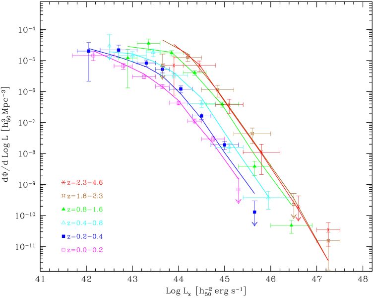
Figure 2: The $1/V_{a}$ estimates of the SXLF in different redshift bins (as labeled) are shown. One sigma error bars are shown for each bin. Important upper limits are shown as downward arrows. The top tick and symbols mark of the upper limit correspond to 2.3 objects (90%) and one object per bin respectively. The solid lines show rough predictions from the best-fit LDDE model (see below) for the redshift bins.

• Unlike previous works (e.g. Boyle et al. 1994; Page et al. 1996; Jones et al. 1997),PLE was absolutely rejected. The 2D K-S probabilities for the best-fit PLE models are less than $10^{-2}$ for all sets of cosmological parameters considered (see Table. 2).

• The best-fit PDE was marginally rejected with a 2D K-S probability of $\approx 5\%$). One difficulty of the best-fit PDE model is that it overproduces the extragalactic soft CXRB intensity.

• The LDDE model, where the evolution rate drops at lower luminosities, gave an acceptable overall description of the SXLF (see below).

The LDDE expression we have used for the overall SXLF is:

$$\frac{{\rm d}\;\Phi\,(L_{\rm x},z)}{{\rm d\;Log}\;L_{\rm x}}={A}\;\left[(L_{\rm x}/{L_{*}})^{{\gamma_{1}}}+(L_{\rm x}/{L_{*}})^{{\gamma_{2}}}\right]^{-1}\cdot e(z,L_{\rm x}),$$ (1)

where $e(z,L_{\rm x})$ is the density evolution factor:

$$\left\{\begin{array}[]{ll}(1+z)^{\max(0,{p1}-{\alpha}({\rm Log}\;{L_{\rm a}}-{\rm Log}\;L_{\rm x}))}&(z\leq{z_{\rm c}};L_{\rm x}<L_{\rm a})\\ (1+z)^{{p1}}&(z\leq{z_{\rm c}};L_{\rm x}\geq L_{\rm a})\\ e({z_{\rm c}},L_{\rm x})\left[(1+z)/(1+{z_{\rm c}})\right]^{{p2}}&(z>{z_{\rm c}})\\ \end{array}\right..$$ (5)

The parameter $\alpha$ represents the degree of luminosity dependence on the density evolution rate for $L_{\rm x}<L_{\rm a}$. The PDE case is $\alpha=0$ and a greater value indicates lower evolution rates at low luminosities.

The best-fit parameters/90% errors for the LDDE model, 2D K-S probabilities $P_{\rm 2DKS}$ (probabilities that the D-value for the 2D K-S statistics exceeds the observed value) are shown in Table 2. The integrated 0.5-2 keV intensity of the model, extrapolated below the survey limit, is also shown. This can be compared with the extragaxlactic CXRB intensity of (7.4–9.0)$\times 10^{-12}[{\rm erg\,s^{-1}\,cm^{-2}\,deg^{-2}}]$, from an update of the ROSAT/ASCA measurements by Miyaji et al. (1998a).

Table 2: The best-fit LDDE Parameters

$(\Omega_{m},\Omega_{\Lambda})$	Parameters/2DKS probability/Intensity
(1.0,0.0)	$A=(1.57\pm.11)\times 10^{-6}$; $L_{*}=0.57^{+.33}_{-.19}$
	$\gamma_{1}=0.68\pm.18$; $\gamma_{2}=2.26\pm.95$; $p1=5.4\pm.4$
	$z_{\rm c}=1.51\pm.15$; $p2=0.0$ (fixed)
	$\alpha=2.3\pm.8$;  ${\rm Log}L_{\rm a}=44.2$ (fixed)
	$P_{\rm 2DKS}$=51%; $I_{\rm x12}=4.5\pm 0.7$
(0.3,0.0)	$A=(2.18\pm.15)\times 10^{-6}$; $L_{*}=0.48^{+.21}_{-.13}$
	$\gamma_{1}=0.58\pm.20$;  $\gamma_{2}=2.26\pm.08$;  $p1=5.8\pm.4$
	$z_{\rm c}=1.54\pm.15$;  $p2=0.0$ (fixed)
	$\alpha=2.6\pm.6$;  ${\rm Log}L_{\rm a}=44.5$ (fixed)
	$P_{\rm 2DKS}$=34%; $I_{\rm x12}=4.8\pm 0.7$
(0.3,0.7)	$A=(2.04\pm.14)\times 10^{-6}$; $L_{*}=0.50^{+.21}_{-.13}$
	$\gamma_{1}=0.58\pm.19$;  $\gamma_{2}=2.27\pm.08$;  $p1=5.8\pm.4$
	$z_{\rm c}=1.51\pm.14$;  $p2=0.0$ (fixed)
	$\alpha=2.9\pm.6$;  ${\rm Log}L_{\rm a}=44.6$ (fixed)
	$P_{\rm 2DKS}$=38%; $I_{\rm x12}=4.6\pm 0.7$
(0.0,0.0)	$A=(2.35\pm.16)\times 10^{-6}$; $L_{*}=0.45^{+.19}_{-.12}$
	$\gamma_{1}=0.56\pm.20$;  $\gamma_{2}=2.24\pm.08$;  $p1=5.9\pm.4$
	$z_{\rm c}=1.55\pm.14$;  $p2=0.0$ (fixed)
	$\alpha=2.7\pm.6$;  ${\rm Log}L_{\rm a}=44.6$ (fixed)
	$P_{\rm 2DKS}$=26%; $I_{\rm x12}=5.3\pm 0.9$

Units – A: [$h_{50}^{3}\;{\rm Mpc^{-3}}$],   $L_{*}$: [$10^{44}\;h_{50}^{-2}{\rm erg\;s^{-1}}$],   $I_{\rm x12}$: $[10^{-12}{\rm erg\,s^{-1}\,cm^{-2}\,deg^{-2}}]$ in 0.5-2 keV

For demonstrations of the goodness of the overall fit, we compare the “flattened”${\rm Log}\;N$ – ${\rm Log}\;S$ ($S^{1.5}N(>S)$) and cumulative $I(<z)$ curves of the real data with the model prediction in Figs. 3 and 4 respectively. The results of the 2DKS test, along with these comparisons show that our overall description is an excellent representation of the current data. The best-fit LDDE models, when extrapolated below the survey limit, gives 50-70% of the extragalactic background in the 0.5-2 keV band considering errors of the fits. If the LDDE parameters are adjusted to produce 90% of the extragalactic 0.5-2 keV background (clusters should contribute $\sim 10\%$), the 2D KS probability drops to $\sim 8\%$.

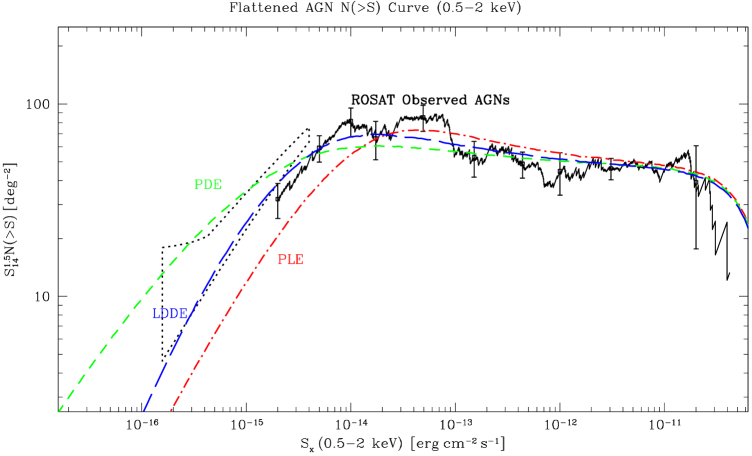
Figure 3: The $S^{1.5}N(>S)$ (a horizontal line corresponds to the Eucleadean slope) curve for our sample AGNs is plotted with 90% errors and are compared with the best-fit PLE (short-dashed), PDE (dot-dashed), and LDDE (dashed) models. The dotted fish is from the fluctuation analysis of the Lockman hole HRI data (including non-AGNs) by Hasinger et al. (1998)

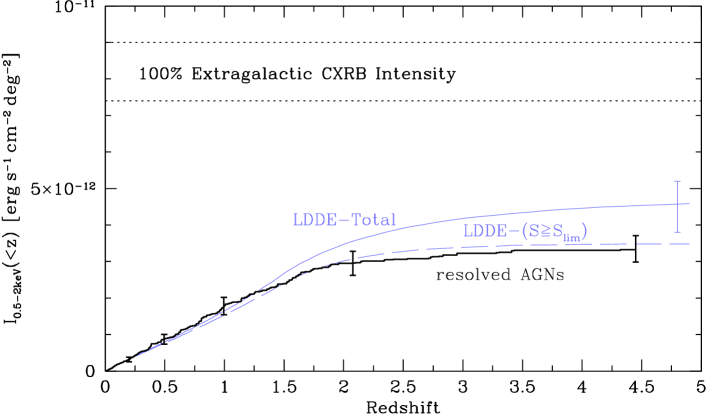
Figure 4: The cumulative intensity $I(<z)$ of the sample AGNs, defined by $\sum_{z_{i}<z}S_{{\rm x}i}/A(S_{{\rm x}i})$, where $S_{{\rm x}i}$ is the flux of the object $i$ and $A(S_{{\rm x}i})$ is the available survey area at this flux (Fig. 1), is plotted as a function of redshift (thick solid line with 90% errors). The best-fit LDDE model is overplotted for the portion represented by the sample ($S\geq S_{\rm lim}=1.9\times 10^{-15}$ $[{\rm erg\,s^{-1}\,cm^{-2}}]$; dashed line) and the total including extrapolation to lower fluxes (thin solid line; with a 90% fitting error). Also the range of the 0.5-2 keV extragalactic background intensity by Miyaji et al. 1998a (updated) is shown.

4 Evolution of QSO Number Density

Number density evolution of luminous QSOs is one of the important pieces of key observational information on understanding blackhole formation and accretion history In particular, we put emphasis on high luminosity QSOs (${\rm Log}\;L>44.5$), where the XLF is consistent with the slope of $\gamma=2.3$ at all redshift and free from complicated luminosity dependence of the evolution rate and contamination from star formation activity.

The comoving number density of the luminous QSOs in our sample are plotted as a function of redshift in Fig. 5. For comparison, number densities (normalized to be approximately equal to the soft X-ray point at $z\sim 2.5$) of optically-selected (Schmidt, Schneider, Gunn 1995, hereafter SSG95) and radio-selected (Shaver et al. 1997) QSOs plotted as a function of redshift (see caption).

Unlike the optical and radio cases, we do not find evidence for decrease of the space density beyond $z\approx 2.7$. Using the maximum-likelihood fitting, we have checked the significance of the inconsistency. Requiring that the number density drops beyond $z=2.7$ as SSG95, the likelihood value (varies as $\chi^{2}$) increased by 3.3, showing that the significance of the inconsistency is 93%, which is marginal. In the $3.0<z\leq 4.6$, we have 5 QSOs in the sample, while expected number in the presence of the decrease like the SSG95 result is 2.4. Including more surveys with a good completeness at the depth of $S_{\rm x}\approx 5\times 10^{-15}$ $[{\rm erg\,s^{-1}\,cm^{-2}}]$ would enable us to discuss whether the soft X-ray selected QSO number density drops beyond $z\approx 3$.

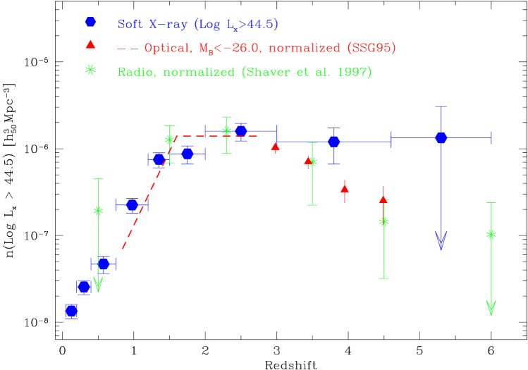
Figure 5: The comoving number density of luminous (${\rm Log}\;L>44.5$) QSOs in our ROSAT AGN sample are plotted as a function of redshift. For comparison, number density of optically-selected ($M_{\rm B}<-26$) (dashed line and filled triangles, from SSG95) and radio-selected (stars, Shaver et al. 1997) QSOs, normalized to the soft X-ray selected QSO number density at $z\sim 2.5$ are overplotted. Error bars are at the 90% confidence level and upper-limits correspond to 1 object per bin at the symbol and 90% at the top.

5 Discussion

There are some discrepancies between our work and previous ones from several authors from combinations of the Einsten Extended Medium Sensitivity Survey (EMSS) and ROSAT surveys (e.g. Boyle et al. 1994; Page et al. 1996; Jones et al. 1997), in that our results are not consistent with PLE. This is partially due to the fact that our combined sample has more AGNs at fainter fluxes, thus better statistics excludes simpler description. However, a direct comparision of the $1/V_{\rm a}$ estimates of the XLF between our sample and that of Jones et al., for example, shows no descrepancy in the $z<0.4$ bin, and high luminosity part (${\rm Log}\;L_{\rm x}\ga 44$) of the $z>0.4$, but descrepancies appear at the low luminosity end of the $z>0.4$ regime. The SXLFs in the regime of bright sources, i.e. the RBS/SA-N based on the RASS for our work and the EMSS sample used by them, are mutually consistent. Thus the uncertainties in conversion of fluxes between ROSAT and Einstein bandpathes do not make significant contributions to the descrepancy. Two likely major causes are: (1) inclusion of apparently narrow-line objects which have indications of AGN activities in our work, while they mainly argue the XLF for broad-line objects. (2): because of the misidentification of the faintest X-ray sources ($S_{\rm x14}\la 0.5$) to field galaxies in their PSPC positioning, they miss some AGNs. A more complete analysis (e.g. comparing redshift distribution) using the original catalogs will be discussed in Miyaji et al. 1998b.

The extrapolations of our best-fit LDDE models explain 50-70% of the 0.5-2 keV extragalactic CXRB, considering errors of the fits. Clusters of galaxies are expected to contribute about 10% in this band. The remaining contributors could be some low-luminosity galaxies/AGNs (${\rm Log}\;L_{\rm x}\la 10^{41.7}$) (see Fig. 2a of Hasinger 1998). These have about the same local volume emissivity as the AGNs in our SXLF, but uncertainties up to by a factor of few may exist, since this low-luminosity galaxy XLF is based on a sample of galaxies nearer than $7.15$ Mpc and the role of local overdensity can be important. Also practically no direct observational information exists for the evolution of these low luminosity sources.

If the low-luminosity galaxies/AGNs contribute significantly to the remaining CXRB, these can be: (1): intrinsically low luminosity AGNs (2) high-intermediate redshift obscured AGNs, which are expected to contribute much of the harder CXRB and redshifted into the ROSAT band. (3): star formation activity.

It is also possible that the behavior of the AGN SXLF (${\rm Log}\;L_{\rm x}\ga 10^{41.7}$) at intermediate-high redshifts does not follow the simple extrapolation of the current LDDE model below the luminosities corresponding to the survey limit at that redshift. Especially our particular formula for the LDDE tends to make the $N(<S)$ drop rapidly below the survey limit. Also the LDDE model-integrated intensity is sensitive to the lowest flux objects in the sample, where incompleteness may play a role. These are fundamental uncertainties in the integrated intensity extrapolated from the best-fit representations of some functional form.

- [1] Appenzeller I., Thiering I. et al. 1998, ApJS, 117, 319
- [2] Bower R.G., Hasinger G. et al. 1996, MNRAS 281,59
- [3] Boyle B.J., Griffiths R.E. et al. 1994, MNRAS 260, 49
- [4] Fasano G., Franceschini A. 1987, MNRAS 225, 155
- [5] Hasinger G. 1998, Astron. Nachr. 319, 37
- [6] Hasinger G.,Burg R., Giacconi R. et al., 1998, A&A 329, 482
- [7] Jones L.R., McHardy I.M. et al. 1997, MNRAS, 285, 547
- [8] Mason K.O. et al. 1998, private communication
- [9] McHardy I.M., Jones L.R. et al. 1998, MNRAS 295, 641
- [10] Miyaji T., Ishisaki Y., Ogasaka, Y. et al. 1998a, A&A 334,13L
- [11] Miyaji T., Hasinger G., Schmidt, M. 1998b, in preparation
- [12] Miyaji T., Hasinger G., Schmidt, M. 1999, Adv. Space Res., submitted
- [13] Page M.J. et al. 1996, MNRAS 281, 579
- [14] Schwope A. et al. 1998, in preparation
- [15] Schmidt M., Schneider D.P., Gunn J.E. 1995, AJ 110, 68 (SSG95)
- [16] Schmidt M., Hasinger G., Gunn J. et al. 1998, A&A 329, 495
- [17] Schmidt M., Giacconi R., Hasinger G. et al. 1999, this volume
- [18] Shaver P.A., Hook I.M., Jackson C.A. et al. 1997, preprint (astro-ph/9801211)
- [19] Zamorani G. et al. 1997, private communication