Correcting for the Effects of Interstellar Extinction

Abstract

This paper addresses the issue of how best to correct astronomical data for the wavelength-dependent effects of Galactic interstellar extinction. The main general features of extinction from the IR through the UV are reviewed, along with the nature of observed spatial variations. The enormous range of extinction properties found in the Galaxy, particularly in the UV spectral region, is illustrated. Fortunately, there are some tight constraints on the wavelength dependence of extinction and some general correlations between extinction curve shape and interstellar environment. These relationships provide some guidance for correcting data for the effects of extinction. Several strategies for dereddening are discussed along with estimates of the uncertainties inherent in each method. In the Appendix, a new derivation of the wavelength dependence of an average Galactic extinction curve from the IR through the UV is presented, along with a new estimate of how this extinction law varies with the parameter $R\equiv A(V)/E(B-V)$. These curves represent the true monochromatic wavelength dependence of extinction and, as such, are suitable for dereddening IR–UV spectrophotometric data of any resolution, and can be used to derive extinction relations for any photometry system.

1. Introduction

A precise knowledge of the wavelength dependence of interstellar extinction (i.e., the absorption and scattering of light by interstellar dust grains) and of any spatial variability in this dependence is important for two distinct reasons. First, the extinction depends on the optical properties of the dust grains along a line-of-sight and potentially can reveal information about the composition and size distribution of the grains. Further, changes in the extinction from place to place may reveal the degree and nature of dust grain processing occurring in the ISM. Second, the wavelength dependence of extinction is required to remove the effects of dust obscuration from observed energy distributions, since most astronomical objects are viewed through at least some small amount of interstellar dust. Spatial variations in the extinction potentially limit the accuracy to which energy distributions can be “dereddened.” Such uncertainties might be acceptably small for very lightly reddened objects, but quickly can become debilitating along modestly reddened sightlines.

This paper follows from a talk given at the meeting “Ultraviolet Astrophysics Beyond the IUE Final Archive” (Fitzpatrick 1998) and addresses the second point raised above, i.e., the correction of energy distributions for the effects of interstellar extinction. The goals are to provide a summary of what is known about the wavelength dependence and spatial variability of interstellar extinction and to present strategies for the best removal of the effects of extinction from astronomical data. In §2, I briefly review the chief features of IR-through-UV extinction and the nature of the known spatial variations. These variations are illustrated with a set of optical/UV extinction curves which span the (currently) known extreme limits of extinction variations. Constraints on the wavelength dependence of extinction and some general correlations between extinction curve shape and interstellar environment are also noted in §2. Strategies for dereddening are discussed in §3 along with estimates of the appropriate uncertainties which ought to be incorporated into an error analysis. Some final comments regarding extinction along extragalactic sightlines and at wavelengths shortward of 1150 Å are given in §4.

The Appendix of this paper describes the construction of a new estimate of the shape of a mean and an environment-dependent IR-through-UV extinction curve. These curves, which may be obtained from the author, are suitable for dereddening multiwavelength spectrophotometric data, such as has become available with the Hubble Telescope’s Faint Object Spectrograph, and for deriving extinction relationships for any photometric system.

2. Spatial Variations in Galactic Extinction

2.1. Variations Abound …

Figure 1 shows several estimates of the shape of a “mean” Galactic extinction curve from the far-IR through the UV region. The curves are presented in a commonly used normalization scheme, $E(\lambda-V)/E(B-V)$, and plotted against inverse wavelength. The significance of the different curves will be discussed later in this paper. For the present, these curves serve to illustrate the overall characteristics of interstellar dust extinction. Typically, the extinction rises through the IR with a power law-like dependence (see Appendix), rolls over slightly in the optical region (“knee”), shows a prominent feature at 2175 Å in the near-UV (“bump”), and has a sometimes steep rise in the far-UV (“fuv rise”). Figure 1 does not attempt to show the relatively narrow optical/IR features which may be associated with interstellar dust, such as the diffuse interstellar bands in the optical or the solid state absorption (or emission) features in the IR (e.g., the 9.8 µm silicate feature).

IR and optical extinction traditionally have been studied using ground based broad- or intermediate- band photometry and sightline-to-sightline variations have been recognized for a long time (e.g., Johnson 1965). These are often characterized using the parameter $R\equiv A(V)/E(B-V)$, i.e., the ratio of total to selective extinction at $V$. The value of $R$ ranges between about 2.2 and 5.8 for sightlines along which UV extinction has also been measured, with a mean value of $\sim$3.1 for the diffuse interstellar medium. It is believed that the shape of the IR extinction law longward of $\sim$8000 Å (the “power law” region) may be invariant and that the observed range in $R$ is due to spatial variations in the steepness of the extinction in the optical region around the “knee” (e.g., Cardelli, Clayton, & Mathis 1989; Martin & Whittet 1990).

Measurements of UV interstellar extinction have relied on satellite or rocket spectrophotometric data, and date back to the original discovery of the 2175 Å bump nearly 30 years ago (Stecher 1969; Bless & Savage 1970). These studies immediately revealed that sightline-to-sightline differences exist within the Galaxy in the detailed properties of UV extinction curves. Important results on the degree of spatial variability of UV extinction were subsequently derived from the large photometric databases accumulated by the TD-1 and ANS satellites (e.g.  Koornneef 1978; Kester 1981; Meyer & Savage 1981).

The most graphic illustrations of spatial variations in UV extinction were provided by the IUE satellite. With its complete spectral coverage between 1150 and 3200 Å and relatively high spectral resolution ($\sim$6 Å in the low-resolution mode) IUE was well-suited for the study of UV extinction and many studies have utilized IUE data to determine the wavelength dependence of extinction along one or more Milky Way lines-of-sight (e.g.  Bohlin & Savage 1980; Witt, Bohlin, & Stecher 1980; Seab, Snow, & Joseph 1981; Morgan, McLachlan, & Nandy 1982; Hecht et al. 1982; Massa, Savage, & Fitzpatrick 1983; Witt, Bohlin, & Stecher 1984; Massa & Savage 1984; Franco, Magazzù, & Stalio 1985; Aiello et al. 1988; and many others). Figure 2 shows analytical representations for $\sim$80 UV extinction curves derived from IUE data (solid curves), illustrating the wide range of properties observed for Galactic UV extinction. These curves are taken from the catalog of Fitzpatrick & Massa (1990), with a few additions, including the lines-of-sight toward HD 210121 (Welty & Fowler 1992) and HD 62542 (Cardelli & Savage 1988). The basis for the analytical representation will be discussed further below.

The overall impression that has come from the last 30 years of extinction studies is that there is a bewildering variety of IR-through-UV extinction curves and that what has often been called “peculiar” extinction is actually quite common. This bodes poorly for the prospects of precisely dereddening astronomical energy distributions. In particular, the range of extinction properties seen in the UV (Figure 2), where the effects of extinction are strongest, may represent a bonanza of information for those who study the properties of interstellar dust grains, but is a potential disaster for those whose main interest in UV extinction is the removal of its effects.

2.2. … But There is Some Order Amid the Chaos

The recognition that interstellar extinction is spatially highly variable is critically important for both the study of dust grains and for the purposes of dereddening. Fortunately for the latter, it has been realized that within the seemingly endless variety of observed extinction curves there are actually some constraints on the wavelength dependence and some links between extinction in the UV, optical, and IR.

This began with Savage (1975) who showed, using OAO-2 satellite data, that the shape of 2175 Å bump can be reproduced well with a Lorentzian profile. This result — which provides important clues about the nature of the 2175 Å feature — allows a functional representation of the bump, and permitted Seaton (1979) to present an estimate of the average Galactic UV extinction curve as a simple analytical formula. This curve is shown in Figure 1 by the dashed curve, extending from 2.7 to 8.7 µm^-1.

Following the lead of Savage and Seaton, Fitzpatrick & Massa (1986, 1988, 1990; collectively referred to hereafter as FM) examined IUE extinction curves for many lines-of-sight and found that all these curves could be fitted extremely well by a single analytical expression with a small number of free parameters. This expression consists of (1) a Lorentzian-like bump term (requiring three parameters, corresponding to bump width $\gamma$, position $x0$, and strength $c3$), (2) a far-UV curvature term (one parameter $c4$), and (3) a linear term underlying the bump and the far-UV (two parameters $c1$ and $c2$). This set of basis functions is shown in Figure 3. With the proper choice of the 6 parameters, essentially all UV extinction curves can be reproduced to within the uncertainties inherent in the data. For most sightlines, this number of free parameters can be reduced to 4, since it has been seen that the position of the 2175 Å bump is nearly invariant and that the intercept and slope of the linear term are tightly correlated (FM; see also Carnochan 1986 and Jenniskens & Greenberg 1993), such that the linear term appears to pivot about the point [$1/\lambda,\frac{E(\lambda-V)}{E(B-V)}$] $\simeq$ [3,2]. The UV portions of the curves shown in Figure 2 ($\lambda<2700$ Å) were all constructed using these functions. There is, thus far, no convincing evidence for substructure in UV extinction curves.

The FM results show that some order underlies the wide spectrum of wavelength dependences seen in the UV, but do not necessarily permit a more accurate dereddening of an object along any given line of sight. Fortunately it has been observed that extinction curves do not vary randomly across the sky, but show distinct regional signatures (e.g., Meyer & Savage 1981; Morgan, McLachlan, & Nandy 1982; Panek 1983; Massa & Savage 1984; Clayton & Fitzpatrick 1987) and it is clear that extinction properties reflect the physical conditions and past processing histories of the environments in which the dust grains reside.

The work of Cardelli, Clayton, & Mathis (1988, 1989; hereafter CCM) provides a link between one measure of dust grain environment and the wavelength dependence of UV-through-IR extinction. CCM found that the shape of UV extinction curves correlates with the parameter $R$ (defined in §2.1 above). This suggests that — although there is considerable scatter — extinction curves from the UV through the IR can be characterized as approximately a one-parameter family dependent on $R$. Thus, if the value of $R$ can be determined (from optical and IR photometry), then the properties of the the entire UV–IR extinction curve can be predicted. The essence of the CCM result is illustrated in Figure 4. Four representative extinction curves are shown, each determined by the value of $R$ listed at the righthand side of the curves. This figure shows that extinction curves which are seen to be very “flat,” or “grey,” in the UV roll over strongly in the optical and are characterized by large values of $R$. Steep UV curves remain steep in the optical and are characterized by small values of $R$. The CCM curve for $R=3.1$ is shown in Figure 1 by the dotted line.

The results of CCM are important in 3 ways: (1) They indicate that some of the spatial variations seen in extinction curves behave coherently and systematically over a wide wavelength range, thus potentially allowing for the consistent dereddening of multiwavelength energy distributions. (2) The observed dependence on $R$ allows for the definition of a meaningful average Galactic extinction curve. Existing datasets of extinction curves, particularly for the UV, are biased toward “interesting” regions where extinction properties are extreme. Computing a simple mean curve from these data does not necessarily yield a reasonable estimate of a Galactic mean. Since it is well-established, however, that the appropriate mean value of $R$ for the diffuse ISM is $\sim$3.1 (e.g., Schultz & Wiemer 1975; Whittet & van Breda 1980; Rieke & Lebofsky 1985), a reasonable definition of a mean Galactic extinction law is that which corresponds to the case where $R=3.1$. (3) They demonstrate a general correlation between dust grain environment and the wavelength dependence of extinction, since large values of $R$ are generally found in dense environments where dust grain growth is thought to occur. The “greyness” of the UV/optical extinction curves for large $R$ is consistent with a larger than normal dust grain population. These results have an important bearing on how to correct for the effects of extinction, discussed in the following section.

3. Correcting for the Effects of Extinction

Given the observed complexity of Galactic UV extinction, what is the best way to deredden an observed energy distribution? There are three different possibilities, which involve the use of a global mean extinction curve, an $R$-dependent curve, and a sightline-specific curve. These three alternatives and their inherent uncertainties are discussed below, and a new derivation of the shape of the average IR-through-UV extinction curve is presented. A more thorough discussion of the uncertainties involved in UV extinction corrections is given by Massa (1987).

3.1. Using a Global Mean Curve

If there is no specific information available about the wavelength dependence of the extinction along a sightline of interest then the only alternative is to adopt some globally defined mean curve and perform a realistic error analysis. This is the least attractive of the three cases discussed here, but is by far the most commonly used. The average Galactic extinction curves from either Seaton (1979; see Figure 1) or Savage & Mathis (1979) are often adopted for dereddening UV data. These should now be superseded by the use of an $R$-dependent curve computed for the case $R=3.1$ (see §2.2). Figure 1 shows the $R=3.1$ curve from CCM (dotted line) and a new determination of the $R=3.1$ case (solid line) which is described in the Appendix to this paper. This new curve aims to reproduce the detailed wavelength dependence of the $R=3.1$ extinction law and has been constructed to account for bandpass effects properly in optical/IR extinction data and to reproduce the observed broad-, intermediate-, and narrow- band extinction measurements. The curve is thus suitable for dereddening multiwavelength spectrophotometric observations and can be used to derive the average extinction relationships in any photometric system.

A complete evaluation of the likely error in a dereddened relative energy distribution $m(\lambda-V)$ requires the propagation of the uncertainty in $E(B-V)$ and the often-neglected but often-dominant uncertainty in the adopted mean curve. This is given by

$$\sigma^{2}_{m(\lambda-V)}=\sigma^{2}_{E(B-V)}\times k(\lambda-V)^{2}+E(B-V)^{2}\times\sigma^{2}_{k(\lambda-V)}$$ (1)

where $k(\lambda-V)$ represents the normalized extinction curve $E(\lambda-V)/E(B-V)$. If absolute fluxes are desired, then the uncertainty in the assumed value of $R$ must also be incorporated (two additional terms on the righthand side of eq. 1, similar to the current terms but with $R$ substituted for $k(\lambda-V)$).

The large database of ANS satellite extinction measurements from Savage et al. (1985) shows that the 1-$\sigma$ scatter at 1500 Å is $\sigma_{k(15-V)}=0.74$, based on $\sim$400 sightlines with $E(B-V)\geq 0.5$. (Only relatively large values of $E(B-V)$ were considered in order to minimize the effects of spectral mismatch error and random noise on the $\sigma$ measurement.) To extend this analysis to other wavelengths, we computed the standard deviation at each wavelength point for the 80 curves shown in Figure 2, and then scaled the result to match the ANS value at 1500 Å. (The actual standard deviation at 1500 Å for the 80 IUE curves is somewhat higher than the ANS result because of the bias in Figure 2 toward extreme extinction curves). The resultant values of $\sigma_{k(\lambda-V)}$ are shown by the thick dotted curve near the bottom of Figure 2 (labeled “$\sigma$”) and are listed at selected wavelengths in the third column of Table 1. This estimate of $\sigma_{k(\lambda-V)}$ should be adopted whenever the average Galactic extinction curve is used for dereddening an observed energy distribution. The uncertainties approach zero for $1/\lambda<3$ $\mu m^{-1}$ due to the curve normalization. The quantity $E(B-V)$ is usually derived directly from photometry and often has an easily quantifiable uncertainty; thus the computation of $\sigma^{2}_{m(\lambda-V)}$ from eq. 1 is straightforward.

Sometimes $E(B-V)$ is not known a priori and is estimated by “ironing out” the 2175 Å extinction bump using an assumed extinction curve shape (e.g., see Massa, Savage, & Fitzpatrick 1983). In many cases, uncertainties in $E(B-V)$ as small as 0.01-0.02 mag for moderately reddened objects have been quoted from this process. This is incorrect! The normalized “height” of the 2175 Å extinction bump — which is the quantity that is important in the ironing-out process — has a 1-$\sigma$ scatter of about $\pm$20% around its mean value (from the data in Figure 2 and Savage et al. 1985). Thus the uncertainty in an $E(B-V)$ measurement derived from the bump must be considered to have a similar relative uncertainty. Since bump strength does not correlate well with other aspects of UV extinction, such as the slope of the linear component or the strength of the far-UV rise (FM), the uncertainty in an energy distribution dereddened this way can be estimated by using eq. 1 with $\sigma_{E(B-V)}\simeq 20\%$ and the values of $\sigma_{k(\lambda-V)}$ from Table 1. The result of this calculation needs to be modified somewhat by removing the signature of the 2175 Å bump. The final estimate of $\sigma^{2}_{m(\lambda-V)}$ computed this way is listed in the last column of Table 1. Multiplying these values by $E(B-V)$ gives the uncertainty in a dereddened relative energy distribution. The values in Table 1 agree well with estimates $\sigma^{2}_{m(\lambda-V)}$ at 1500, 1800, 2200, 2500, and 3300 Å derived from the ANS data of Savage et al (1985), and are consistent with the analysis of Massa (1987).

3.2. Using a $R$-Dependent Mean Curve

If the value of $R$ has been measured along a sightline of interest, or if some general information is available about the dust grain environment (e.g., dense region or diffuse region?), then the uncertainties in dereddening can be reduced somewhat by adopting an $R$-dependent extinction curve computed at the appropriate value of $R$. For the original 29 sightlines used by CCM, the standard deviation of the individual observed extinction curves minus the computed $R$-dependent curves is about a factor of 2 smaller than when the individual curves are compared to the average Galactic ($R=3.1$) curve. Thus the uncertainties in a dereddened energy distribution can be estimated using eq. 1 and adopting 0.5 times the $\sigma_{k(\lambda-V)}$ values from Table 1. If $R$ is poorly measured or only estimated from environmental factors, then allowance must be made for this in the error analysis.

Using an appropriate $R$-dependent curve can slightly improve the accuracy of results from ironing out the 2175 Å bump. The values of $\sigma^{2}_{m(\lambda-V)}$ can be estimated as above in §3.1, using the same value of $\sigma_{E(B-V)}\simeq 20\%$ and 0.5 $\times$ $\sigma_{k(\lambda-V)}$ from Table 1. The resultant values of $\sigma^{2}_{m(\lambda-V)}$ are about 85% as large as those listed in the last column of Table 1. The gain from using the $R$-dependent curves is only marginal because the normalized bump heights are highly variable and not correlated with $R$.

It is important to note that, even when $R$ and $E(B-V)$ are well-determined, the use of an $R$-dependent extinction curve only reduces — but does not eliminate — the wavelength dependent dereddening error. The standard deviation of the observed vs. $R$-dependent curves does not go to zero, even for the sample of 29 sightlines used by CCM to define the $R$-dependence, because the UV/optical curves are not really a one-parameter family dependent only on $R$. Curves derived for different sightlines with the same values of $R$ show a wide range of properties, including differences in the strengths of the bump and the far-UV rise. Thus, as noted by CCM, the CCM formula reproduces a general trend, but does not provide particularly good fits to individual extinction curves, even when the value of $R$ is well-determined.

Apart from this intrinsic scatter around the mean $R$ relation, the accuracy of the CCM results is limited in the IR/optical region due to bandpass effects with the broadband Johnson filters used to measure the extinction. As a result, CCM tends to overestimate the level of extinction in the near-IR and blue-visible. In the Appendix, a new derivation of the $R$-dependence of IR-through-UV extinction is presented. This corrects for the systematic bandpass effects in CCM, but is still plagued by the same uncertainties caused by the “cosmic” scatter of extinction properties around the mean $R$ relation.

3.3. Using a Sightline-Specific Curve

Without question, the best of all possible dereddening choices is to use an extinction curve derived explicitly for the sightline of interest. This advice is not so unhelpful as it may sound, because the archives of the IUE satellite may well contain normal stars in the direction (and at the distance) of the object of interest, from which extinction curves may be derived (e.g., halo stars in the case of extragalactic sightlines). The accuracy of the dereddened energy distribution may thus be limited chiefly by the uncertainties in the “pair method” of constructing the extinction curve (see, e.g., Massa et al. 1983) and by the determination of $E(B-V)$ for the object of interest. For a well-determined curve, “ironing out” the bump — in the cases when $E(B-V)$ is not known explicitly — should yield the same degree of accuracy as for the cases when $E(B-V)$ is known a priori. An example of such an approach is the determination of the intrinsic energy distributions of rare or exotic objects located in clusters with more mundane objects. Massa & Savage (1985) utilize this technique, using extinction curves derived from main sequence B stars in open clusters to determine the continuum shapes of cluster O stars.

4. Final Comments

The results discussed above strictly pertain to Milky Way extinction for wavelengths longward of about 1150 Å (the IUE satellite cutoff). Observers of extragalactic objects must contend with foreground Milky Way extinction as well as extinction due to dust grains local to the object of interest. It is reasonable to assume that the properties of interstellar extinction in external galaxies are fully as complex as found for the Milky Way. However, only for the nearby Large Magellanic Cloud (LMC) do observed extinction curves for individual sightlines approach the accuracy needed to study spatial extinction variations (see Fitzpatrick 1998 and references within). The properties of Milky Way extinction along the high galactic latitude sightlines relevant to most extragalactic observations are also not well-determined. One of the few quantitative studies of high latitude extinction, that by Kiszkurno-Koziej & Lequeux (1987) utilizing ANS satellite data, suggests that halo extinction is slightly steeper in the far-UV and has a weaker 2175 Å bump than the typical extinction found in the plane of the Galaxy. Attempts to eliminate galactic foreground reddening by ironing out the bump may lead to systematic underestimates of the total amount of foreground extinction.

The properties of extinction in the wavelength range 912-1150 Å are poorly known, but the work that has been done (e.g., York et al. 1973; Snow, Allen, & Polidan 1990) suggests that the far-UV rise continues at least down to wavelengths of 950 Å or so. An intrinsic problem with measuring extinction in this wavelength range is the high density of H I and H₂ absorption lines which mimic continuous absorption in low-resolution data. CCM suggest that the wavelength dependence of extinction in this region is reasonably well-represented by an extrapolation of the fitting functions used in the IUE wavelength range. At the present, the best dereddening strategy for 912-1150 Å data would be to adopt such an extrapolation, based if possible on IUE extinction curves derived for the sightline of interest. The uncertainties listed in Table 1 for 1000 Å are based on this simple extrapolation.

Appendix A Deriving a $R$-Dependent IR-through-UV Extinction Curve

In this Appendix a new estimate of the wavelength dependence of Milky Way extinction from the IR through the UV is derived. The motivation for this is the need for a multiwavelength extinction curve suitable for dereddening IR-through-UV spectrophotometric data now available from, for example, the Hubble Space Telescope’s Faint Object Spectrograph (see, e.g., Fitzpatrick & Massa 1998 and Guinan et al. 1998). The specific goals are 1) to produce a curve for the $R=3.1$ case which reproduces existing narrow band extinction measurements and the principal Johnson and Strömgren photometric extinction relations and 2) to define the $R$-dependence of the extinction law, relying principally on spectral regions where this dependence is well-determined. Existing estimates of the average wavelength dependence of optical/near-IR extinction do not accurately portray the true shape of the curve due to bandpass effects arising from the broadband photometry used to derive the curves. This deficiency will be corrected by using synthetic photometry.

A.1. The UV Region

CCM noted a correlation between the value of $R^{-1}$ (as determined from IR/optical photometry) and the values of $A(\lambda)/A(V)$ (i.e., total extinction at $\lambda$ normalized by total extinction at V) at UV wavelengths using parametrized extinction curves for a subset of 29 stars from the FM sample. They consequently derived a complex polynomial expression to reproduce the wavelength- and $R$- dependences. We approach the problem slightly differently and note that the essence of the CCM result is two correlations involving the coefficients of the FM fitting function originally used to parametrize the extinction curves studied by CCM. We thus derive the functional forms of these correlations and retain the FM fitting function to compute the values of $E(\lambda-V)/E(B-V)$ for wavelengths $\lambda<2700$ Å.

Figure 5 illustrates the two correlations. The top panel shows a plot of the FM parameter $c2$ (representing the slope of the linear UV extinction component) vs. $R^{-1}$ (filled circles) along with a least squares estimate of the linear relationship between the two (dashed line). The data are for a subset of the FM sample for which IR photometry could be used to deduce the value of $R$ (see below), with the addition of the sightline toward HD 210121 (Welty & Fowler 1992; Larson, Whittet, & Hough 1996). This represents the only convincing correlation between $R$ and the properties of the UV extinction curve (see, e.g., Jenniskens & Greenberg 1993). The equation of the least-squares fit to the data is

$$c2=-0.824+4.717\times R^{-1}\\$$ (A1)

No physical interpretation or significance is placed on the form of the adopted functional relationship between $R$ and $c2$; it is merely that which best reproduces the observed correlation. We note, however, that the intrinsic slope of extinction in the optical region is proportional to $R^{-1}$, and that eq. A1 thus simply implies that the slopes of the extinction curves in the UV and optical vary together in a linear manner — as optical extinction steepens, UV extinction steepens.

The bottom panel of Figure 5 shows the well-known relationship between slopes ($c2$) and intercepts ($c1$) of the linear background component (FM; Carnochan 1986; Jenniskens & Greenberg 1993). The data are for the full set of 80 curves from FM, plus HD 210121, and minus the Orion Nebula stars (HD 36982, 37022, 37023, and 37061) which suffer from scattered light contamination (which mainly affects the linear intercept). The equation of the least squares fit to this relationship (dashed line), is

$$c1=2.030-3.007\times c2\\$$ (A2)

We use the following mean values for the other four parameters required to specify UV extinction curves with the FM formula: $x0$ (bump position) = 4.596 µm^-1; $\gamma$ (bump width) = 0.99 µm^-1; $c3$ (bump strength) = 3.23; and $c4$ (FUV curvature) = 0.41.

A.2. The Optical/IR Region

A common way of representing the wavelength dependence of extinction in the optical and IR regions is to draw a smooth curve through the values of $E(\lambda-V)/E(B-V)$ (or some other curve normalization) derived from Johnson UBVRIJHKLM photometry, assuming that these represent the monochromatic values of the extinction at the filter effective wavelengths $\lambda_{eff}$ (e.g., CCM, Martin & Whittet 1990). This procedure does not accurately yield the monochromatic extinction curve because it ignores the wavelength dependence of extinction across the width of an individual filter. Extinction decreases towards longer wavelengths in the optical/IR region and therefore the value of $\lambda_{eff}$ for a reddened star is shifted to a longer wavelength than for an identical unreddened star. An extinction measurement made by comparing photometric indices for two such stars (i.e., the “pair method”) will always overestimate the monochromatic extinction in the neighborhood of $\lambda_{eff}$ because stellar emergent fluxes in the optical/IR decrease towards longer wavelengths (for early-type stars). The magnitude of this effect depends on how much the true extinction curve varies across the filter. A broadband $E(\lambda-V)/E(B-V)$ measurement will also be influenced by the intrinsic energy distributions of the stars used in the pair method and by the total amount of extinction.

The approach taken here is to find the wavelength dependence of the optical/IR extinction curve which reproduces the photometric extinction measurements when synthetic photometry of an artificially reddened stellar energy distribution is compared with that of identical but unreddened star. To represent the stellar energy distribution, an ATLAS9 model atmosphere from R.L. Kurucz (with $T_{eff}=30000$ K and $\log g=4.0$) is used, along with an adopted value of $E(B-V)=0.5$. Synthetic photometry is performed to yield measurements in the broadband Johnson UBVRIJHKLM system and the intermediate band Strömgren uvby system. The first step is to determine the curve shape for the mean $R=3.1$ case and then to define the nature of the variation with $R$. The first two columns of Table 2 list the photometric extinction ratios (in both the Johnson and Strömgren systems) and their observed values, which the $R=3.1$ extinction curve is required to reproduce. References to the observations are given in Column 3. In addition, the curve is constrained to reproduce the mean narrowband measurements in the 3400–7900 Å region published by Bastiaansen (1992), which are assumed to represent the monochromatic values of the extinction for the case $R=3.1$ at the filter central wavelengths.

Figure 6 shows the shape of the monochromatic extinction curve which best satisfies these requirements (thick solid curve), plotted as total extinction $A(\lambda)$ normalized by $E(B-V)$. The arbitrarily scaled profiles of the Johnson and Strömgren filters are indicated, and the Bastiaansen data shown by the small plus signs (“+”). The agreement between the $R=3.1$ curve and the Bastiaansen data is clear from the figure. The fourth column of Table 4 gives the values of the photometric extinction ratios produced by the curve, also in very good agreement with the observations.

For wavelengths longward of 2700 Å($1/\lambda<3.7\mu$m^-1), the $R=3.1$ curve is defined by a cubic spline interpolation between a set of optical/IR anchor points (filled circles) and a pair of UV anchor points (filled squares). The values of the UV anchors (at 2700 Å and 2600 Å) are determined by the FM fitting function for the case $R=3.1$ (see above) and assure a smooth junction between the optical and UV regions at 2700 Å. The anchor at 0 µm^-1 is fixed at 0 (i.e., no extinction at infinite wavelength) and the values of the other six optical/IR points were adjusted iteratively to find the curve shape which best reproduced the extinction observations. The wavelengths chosen for the spline anchor points are somewhat arbitrary, although points in the IR, the optical normalization region, and the near-UV are clearly required. The wavelengths and values of the spline anchors for the $R=3.1$ curve are given in Table 3.

Note the slope of the derived extinction curve does not approach zero as $1/\lambda$ approaches zero. We sacrificed this physically expected requirement in order to achieve a better fit to the Johnson IR photometry and to preserve the simplicity of the fitting procedure. A zero slope could have been guaranteed by, for example, adopting a power law to represent the extinction; but no single power law can reproduce the IR photometry to an acceptable level. The new curve should be treated as very approximate at wavelengths beyond the limit of the M band (i.e., at $\lambda>6\micron$).

The overall $R$-dependence of the optical/IR curve is relatively easy to incorporate by the following adjustments in the spline anchors: (1) the UV points are computed by the FM fitting function using the coefficient values given above, including the $R$-dependent value of $c2$; (2) the IR points at $1/\lambda<1$µm^-1 are simply scaled by $R$/3.1, since the shape of the far-IR extinction is believed to be invariant (see §2.1 and below); and (3) the optical points are vertically offset by an amount $R-3.1$, with slight corrections made to preserve the normalization. Without these corrections (which are less than 0.015 over the range $R$ = 2 to 6) the extinction curves would drift away from the standard normalization, i.e., $E(B-V)=1$, by a few hundredths of a magnitude as $R$ departed from the value 3.1. Table 4 gives formulae for computing the $R$-dependent values of the optical spline anchors. The corrections just noted are manifested in the departure of the linear term from a value of 1.0 and in the higher order term for the 4110 Å point.

It is not obvious a priori that the above adjustments in the spline should produce the proper curve shapes in the relatively large gaps between the 4 points in the optical normalization region and the UV or IR regions. However, it will be shown below that the resultant curves are in good agreement with observations.

A.3. The Full R-Dependent Curve

Figure 7 shows the full wavelength range of the IR-through-UV $R$-dependent extinction curves derived here, for four representative values of $R$ (thick solid and dashed lines). For $\lambda\leq 2700$ Å the curves are computed using the FM fitting function and for $\lambda>2700$ Å the curves are spline interpolations between the $R$-dependent spline anchors. The CCM results are shown for comparison by the thin dotted lines for the same four $R$ values. In the UV region, the new results and the CCM curves are similar for $R\leq$ $\sim$4.0, but diverge for larger $R$. The main reason for this discrepancy lies in the UV linear extinction component. While CCM adopted a linear relationship between the slope $c2$ and intercept $c1$, their relation — shown by the dotted line in the bottom panel of Figure 5 — does not agree well with the observations. The large discrepancy at small values of $c2$ (i.e., large $R$) produces the difference seen in Figure 7.

A closeup comparison between the new results and CCM in the optical/IR region for the $R=3.1$ case can be seen in Figure 6, where the CCM curve is indicated by the dotted line. The disagreement in the region near the Johnson $R$ filter illustrates the bandwidth effect discussed above. The CCM curve is fixed at $A(\lambda)/E(B-V)=2.32$ at 7000 Å, which is taken as $\lambda_{eff}$ for the Johnson $R$. The new curve is constructed to yield the same value of $A(\lambda)/E(B-V)$ but for synthetic photometry with the Johnson $R$. The discrepancy is particularly large for this filter because of the steep change in extinction across its relatively broad profile. This effect also accounts for the lesser discrepancies in the regions of the $U$, $B$, $I$, and $J$ filters. O’Donnell (1994) presented a revision to the CCM formula in the region of the $U$, $B$, and $V$ filters based on the Strömgren photometric indices. This revision uses the same stategy as CCM of fixing the extinction ratios at the filter effective wavelengths, but more closely resembles the newly derived monochromatic extinction curve because the bandwidth effects in the narrower Strömgren filters are smaller.

Note that the technique used here to produce $R$-dependent curves can be used to construct “customized” UV/optical extinction curves for sightlines with well-defined UV extinction properties. It is simply necessary to substitute the measured values of $A(\lambda)/E(B-V)$ at 2700 Å and 2600 Å for the UV spline anchors listed in Table 3 and then perform the cubic spline interpolation to determine the optical portion of the curve, which smoothly joins the measured UV curve at 2700 Å. This method was used in Figure 2 to extend the IUE curves into the optical region.

The assertion that the shape of the IR extinction law is invariant can be tested by comparing results obtained from the $R$-dependent curves in Figure 7 — which were constructed based on this assumption — with observations. This comparison is made in Table 5 for a number of sightlines which span the observed range in $R$. The “model” data listed for each sightline are the results from synthetic photometry on model stellar energy distributions artificially reddened using the $R$-dependent curves, with $E(B-V)$ values from column 2 of the table and $R$ values from column 7. The listed values of $R$ are those that best reproduce the observed color excesses and the uncertainties result from assuming uncertainties of $\pm$0.02 mag in $E(B-V)$ and $\pm$0.05 mag in the IR $E(V-\lambda)$. The agreement between observations and model values is excellent and there are no strong systematic trends evident. The results are thus consistent with an invariant IR extinction curve. At wavelengths greater than $\sim$1 µm, the extinction curve roughly resembles a power law with an index of $\sim$1.5. This is similar to that adopted by CCM (1.6), but much flatter than that of Martin & Whittet (1990; $\sim$1.8).

Values of $R$ are sometimes estimated from the relation $R\simeq 1.1\times E(V-K)/E(B-V)$. Exact relationships between R and the IR color excesses can be derived for the new $R$-dependent curves. These are given by

$$R=1.39\times\frac{E(V-J)}{E(B-V)}-0.02\\$$ (A3)

$$R=1.19\times\frac{E(V-H)}{E(B-V)}+0.04\\$$ (A4)

$$R=1.12\times\frac{E(V-K)}{E(B-V)}+0.02\\$$ (A5)

$$R=1.07\times\frac{E(V-L)}{E(B-V)}-0.01\\$$ (A6)

The coefficients in each of these equations actually depend on the value of E(B-V) itself but, over the range $E(B-V)=0$ – 2.0, vary by only several hundredths. The values in the equations are the results for $E(B-V)=0.5$.

At the blue end of the optical region, the interpolation between the optical and UV spline anchor points can be tested by comparing predictions of the extinction indices $E(U-B)/E(B-V)$ and $E(c1)/E(b-y)$ with photometric measurements. Figure 8 shows this comparison, with the difference between the observed values and predicted values — derived from synthetic photometry of “customized” extinction curves from the FM sample — plotted against the slope of the linear component $c2$. The curves were produced as described above, by adopting the observed values of $A(\lambda)/E(B-V)$ at 2600 Å and 2700 Å as the UV anchor points. The random scatter (measurement noise) in both indices is large, but no systematic trends are seen and the model curves appear to reproduce at least the integrated properties of extinction well in the near-UV region. Over the range of $c2$ values shown, the model values of $E(U-B)/E(B-V)$ range from about 0.6 to 0.8 and the values of $E(c1)/E(b-y)$ from about 0.0 to 0.3.

In summary, the $R$-dependent curves derived here reproduce existing photometric and spectrophotometric measurements and provide a good estimate of the true monochromatic wavelength dependence of interstellar extinction in the IR-through-UV regions. These curves should be preferred for dereddening UV, optical, and near-IR spectrophotometry. Since the new curves give the detailed wavelength dependence of extinction, they can be used to predict the extinction relationships for any photometric system by using synthetic photometry of artificially reddened energy distributions. An IDL procedure to produce the new curves at any desired value of $R$ and over any wavelength range can be obtained from the author or via anonymous ftp at astro1.vill.edu. After logging in, change directories to pub/fitz/Extinction, and download the file “FMRCURVE.pro.” Alternatively, this directory contains a series of compressed files named “FMRCURVEn.n.txt” (e.g., “FMRCURVE3.1.txt”) which contain ASCII versions of the curves for various values of $R$ (“n.n”). Two columns of data are contained in each file; the first contains wavelengths in Å and the second contains the extinction curve in $A(\lambda)/E(B-V)$. There are 1099 sets of points in each file.

Table 1Uncertainties in Extinction Corrections

		$\sigma_{k(\lambda-V)}$	$\sigma_{m(\lambda-V)}/E(B-V)$
Wavelength	$\lambda^{-1}$	(for corrections using	(for “ironing out”
(Å)	($\mu m^{-1})$	average Galactic curve)	the 2175 Å bump)
(1)	(2)	(3)	(4)
1000	10.0	2.50	3.80
1100	09.1	1.70	2.80
1200	08.3	1.30	2.10
1300	07.7	1.00	1.70
1400	07.1	0.86	1.50
1500	06.7	0.74	1.30
1600	06.2	0.66	1.10
1800	05.6	0.55	1.00
2000	05.0	0.55	0.89
2200	04.5	0.64	0.78
2400	04.2	0.43	0.69
2600	03.8	0.30	0.62
2800	03.6	0.23	0.55
3000	03.3	0.17	0.48
3500	02.9	0.06	0.35
4000	02.5	0.00	0.25

Table 2Optical/IR Extinction Ratios for R=3.1

Extinction	Observed		Model Curve
Ratio	Value	Reference	Value
(1)	(2)	(3)	(4)
$A(M)/E(B-V)$	$\phantom{string}0.08-0.12$	1,2	$\phantom{string}0.12$
$A(L)/E(B-V)$	$\phantom{string}0.09-0.20$	1,2,3,4	$\phantom{string}0.19$
$A(K)/E(B-V)$	$\phantom{string}0.33-0.38$	2,3,4	$\phantom{string}0.36$
$A(H)/E(B-V)$	$\phantom{string}0.52-0.55$	1,2	$\phantom{string}0.53$
$A(J)/E(B-V)$	$\phantom{string}0.85-0.91$	1,2,3	$\phantom{string}0.86$
$A(I)/E(B-V)$	$\phantom{string}1.50$	3	$\phantom{string}1.57$
$A(R)/E(B-V)$	$\phantom{string}2.32$	3	$\phantom{string}2.32$
$A(V)/E(B-V)$	$\phantom{string}3.10$		$\phantom{string}3.10$
$E(U-B)/E(B-V)$	$\phantom{string}0.70+0.05\times E(B-V)$	5	$\phantom{string}0.69+0.04\times E(B-V)$
$E(b-y)/E(B-V)$	$\phantom{string}0.74$	6	$\phantom{string}0.74$
$E(m1)/E(b-y)$	$-0.32$	6	$-0.32$
$E(c1)/E(b-y)$	$\phantom{string}0.20$	6	$\phantom{string}0.17$
$E(u-b)/E(b-y)$	$\phantom{string}1.5$	6	$\phantom{string}1.54$

Table 3Cubic Spline Anchor Points for R = 3.1 Curve

Wavelength	$\lambda^{-1}$	$A(\lambda)$
(Å)	(µm-1)	$E(B-V)$
(1)	(2)	(3)
$\infty$	0.000	0.000
26500	0.377	0.265
12200	0.820	0.829
06000	1.667	2.688
05470	1.828	3.055
04670	2.141	3.806
04110	2.433	4.315
02700	3.704	6.265
02600	3.846	6.591

Table 4R-Dependent Values of Optical Spline Anchor Points

Wavelength	$\lambda^{-1}$	$A(\lambda)$
(Å)	(µm-1)	$E(B-V)$
(1)	(2)	(3)
6000	1.667	$-0.426+1.0044\times R$
5470	1.828	$-0.050+1.0016\times R$
4670	2.141	$\phantom{string}0.701+1.0016\times R$
4110	2.433	$\phantom{string}1.208+1.0032\times R-0.00033\times R^{2}$

Table 5Comparison of Model IR Color Excesses With Observations

	$E(B-V)$	$E(V-J)$	$E(V-H)$	$E(V-K)$	$E(V-L)$
Sightline	(mag)	(mag)	(mag)	(mag)	(mag)	$R$
(1)	(2)	(3)	(4)	(5)	(6)	(7)
HD 210121 — observed	0.38	0.64	0.71	0.73	0.78	$\cdots$
HD 210121 — model	$\cdots$	0.61	0.70	0.75	0.79	$2.22\pm 0.14$
HD 021483 — observed	0.55	1.07	1.22	1.32	1.40	$\cdots$
HD 021483 — model	$\cdots$	1.08	1.23	1.31	1.39	$2.69\pm 0.11$
HD 167771 — observed	0.44	0.96	1.14	1.23	1.25	$\cdots$
HD 167771 — model	$\cdots$	0.98	1.13	1.20	1.27	$3.10\pm 0.16$
HD 147889 — observed	1.09	2.98	3.52	3.90	4.11	$\cdots$
HD 147889 — model	$\cdots$	3.11	3.58	3.81	4.04	$3.92\pm 0.17$
HD 037061 — observed	0.54	1.74	2.05	2.21	2.34	$\cdots$
HD 037061 — model	$\cdots$	1.78	2.06	2.19	2.32	$4.57\pm 0.18$
HD 038087 — observed	0.33	1.10	1.45	1.58	1.53	$\cdots$
HD 038087 — model	$\cdots$	1.21	1.40	1.49	1.57	$5.08\pm 0.58$
HD 036982 — observed	0.34	1.38	1.61	1.85	$\cdots$	$\cdots$
HD 036982 — model	$\cdots$	1.43	1.66	1.76	$\cdots$	$5.83\pm 0.57$

Note. — Observed color excesses are derived using the intrinsic colors from Wegner 1994. Model color excesses are computed via synthetic photometry of artificially reddened stellar energy distributions using the IR extinction law derived in the Appendix and assuming the $E(B-V)$ values from column 2 and the $R$ values from column 7. The stated values of $R$ yield the best fits to the observed IR color excesses and the uncertainties are based on the assumptions $\sigma_{E(B-V)}=0.02$ and $\sigma_{E(V-\lambda)}=0.05$. Kurucz ATLAS9 models with appropriate values of $T_{eff}$ were used to represent the intrinsic stellar energy distributions.

Figure 1.— Normalized interstellar extinction curves from the far-IR through the UV. Several general features of the curves are noted. The solid and dotted curves are estimates for the case $R\equiv A(V)/E(B-V)=3.1$ derived in the Appendix of this paper and by Cardelli, Clayton, & Mathis 1989, respectively. The dashed curve shows the average Galactic UV extinction curve from Seaton 1979.

Figure 2.— Examples of 80 Galactic UV extinction curves derived from IUE satellite observations. Analytical fits to the curves are shown, based on the work of Fitzpatrick & Massa 1990. The curves are taken from the Fitzpatrick & Massa catalog, with the addition of the lines-of-sight toward HD 210121 from Welty & Fowler 1992 and HD 62542 from Cardelli & Savage 1988. This figure demonstrates the enormous range of properties exhibited by UV extinction in the Milky Way. The dotted line, labeled “$\sigma$,” shows the standard deviation of the sample scaled to the value $\sigma(1500\AA)=0.74$, as derived from ANS satellite data (see §3.1).

Figure 3.— Analytical fitting functions for UV extinction curves from Fitzpatrick & Massa 1990. A normalized UV extinction curve (thick solid curve) can be represented by a combination of three functions: (1) a linear background component (thin dashed line), (2) a UV bump component (thin solid curve), and (3) a far-UV curvature component (thin dotted line). The linear background is parameterized by two tightly correlated coefficients (slope and intercept), the bump by three coefficients (strength, width, and central position), and the far-UV curvature by a single scale factor. Given the near invariance in bump central position and the correlation between the linear coefficients, most Galactic UV extinction curves can be reproduced to within the observational uncertainties with only four free parameters.

Figure 4.— Far-IR through UV extinction curves from Cardelli, Clayton, and Mathis 1989 (CCM). CCM found that extinction curves can be expressed approximately as a 1-parameter family that varies linearly with $R^{-1}$, where $R\equiv A(V)/E(B-V)$ and has a mean value in the diffuse interstellar medium of 3.1. Examples of CCM’s results are shown for four representative values of $R$, listed on the righthand side of the figure next to the corresponding curve.

Figure 5.— Left Panel: Slope of the UV linear extinction component $c2$ plotted against $R^{-1}$ (filled circles) for 31 sightlines from the Fitzpatrick & Massa 1990 (FM) sample plus HD 210121 (at $R^{-1}=0.45$). The adopted linear relationship between these quantities is indicated with the dashed line and given by $c2=-0.824+4.717R^{-1}$. Right Panel: Intercept of the UV linear extinction component $c1$ plotted against the linear slope $c2$ (filled circles) for the full set of $\sim$80 extinction curves from the FM catalog. The adopted linear relationship between these parameters is indicated by the dashed line and given by $c1=2.030-3.007c2$. The relationship between $c1$ and $c2$ implicit in the CCM formula is shown by the dotted line.

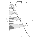
Figure 6.— A new estimate of the wavelength dependence of extinction in the IR/optical region for the case $R=3.1$ (thick solid curve). Plus signs represent the extinction data from Bastiaansen 1992, normalized to $R=3.1$; the dotted line shows the CCM curve for $R=3.1$. The arbitrarily scaled profiles of the Johnson UBVRIJHKLM and Strömgren uvby filters are shown for comparison. The new curve was constrained to reproduce the broad- and intermediate-band filter-based extinction measurements listed in Table 2 and to fit the Bastiaansen data. For $\lambda>2700$ Å ($1/\lambda<3.7\micron^{-1}$) the curve is constructed as a cubic spline interpolation between the points marked by the filled symbols (see Table 3). At wavelengths shortward of 2700 Å, the curve is computed using the FM fitting function with the coefficients given in the Appendix.

Figure 7.— Examples of the $R$-dependent far-IR through UV extinction curves derived in this paper (thick solid and dashed curves). The corresponding values of $R$ are listed on the righthand side of the figure beside the curves. For comparison, the results of CCM for the same four values of $R$ are shown.

Figure 8.— Left Panel: Observed-minus-predicted values of $E(U-B)/E(B-V)$ plotted against the slope of the UV linear extinction component $c2$ (filled circles) for sightlnes from the FM sample. Model values of $E(U-B)/E(B-V)$ vary over the range $\sim$0.6 to $\sim$0.8 for the observed range in $c2$. Right Panel: Observed minus predicted values of the Strömgren extinction ratio $E(c1)/E(b-y)$ plotted against $c2$ (filled circles) for the FM sightlines with Strömgren data. Model values of $E(c1)/E(b-y)$ vary over the range $\sim$0.0 to $\sim$0.3 for the observed range in $c2$.

References

- Aiello, et al. (1988) Aiello, S., Barsella, B., Chlewicki, G., Greenberg, J.M., Patriarchi, P., & Perinotto, M. 1988, A&AS, 73, 195
- Bastiaansen (1992) Bastiaansen, P.A. 1992, A&AS, 93, 449
- Bless & Savage (1970) Bless, R.C., & Savage, B.D. 1970, Observations of Interstellar Extinction in the Ultraviolet with the OAO Satellite. In: Houziaux, L. & Butler, H.E. (eds.) Proc. IAU Symp. 36, Ultraviolet Stellar Spectra and Related Ground-Based Observations. Springer-Verlag, New York, p. 28
- Bohlin & Savage (1980) Bohlin, R.C., & Savage, B.D. 1980, ApJ, 249, 109
- Cardelli et al. (1988) Cardelli, J.A., Clayton, G.C., & Mathis, J.S. 1988, ApJ, 329, L33
- Cardelli et al. (1989) Cardelli, J.A., Clayton, G.C., & Mathis, J.S. 1989, ApJ, 345, 245 (CCM)
- Cardelli & Savage (1988) Cardelli, J.A., & Savage, B.D. 1988, ApJ, 325, 864
- Carnochan (1986) Carnochan, D.J. 1986, MNRAS, 219, 903
- Clayton & Fitzpatrick (1987) Clayton, G.C., & Fitzpatrick, E.L. 1987, AJ, 92, 157
- Crawford (1975) Crawford, D.L. 1975, PASP, 87, 481
- FitzGerald (1970) FitzGerald, M.P. 1970 A&A, 4, 234
- Fitzpatrick (1998) Fitzpatrick, E.L. 1998, in “Ultraviolet Astrophysics, Beyond the IUE Final Archive,” eds. R. Gonzalez-Riestra, W. Wamsteker, and R. Harris (ESA SP-413), p. 461
- Fitzpatrick & Massa (1986) Fitzpatrick, E.L., & Massa, D.L. 1986, ApJ, 307, 286
- Fitzpatrick & Massa (1988) Fitzpatrick, E.L., & Massa, D.L. 1988, ApJ, 328, 734
- Fitzpatrick & Massa (1990) Fitzpatrick, E.L., & Massa, D.L. 1990, ApJS, 72, 163
- Fitzpatrick & Massa (1998) Fitzpatrick, E.L., & Massa, D.L. 1998, in preparation
- Franco et al. (1985) Franco, M.L., Magazzù, A., & Stalio, R. 1985, A&A, 147, 191
- Guinan et al. (1998) Guinan, E.F. et al. 1998, ApJ, in preparation
- Hecht et al. (1982) Hecht, J., Helfer, H.L., Wolf, J., Donn, B., & Pipher, J.L. 1982, ApJ, 263, L39
- Jenniskens & Greenberg (1993) Jenniskens, P., & Greenberg, J.M. 1993, A&A, 274, 439
- Johnson (1965) Johnson, H.L. 1965, ApJ, 141, 923
- Kester (1981) Kester, D. 1981, A&A, 99, 375
- Kiszkurno-Koziej & Lequeux (1987) Kiszkurno-Koziej, E., & Lequeux, J. 1987, A&A, 185, 291
- Koornneef (1978) Koornneef, J. 1978, A&A, 68, 139
- Larson, Whittet, & Hough (1996) Larson, K.A., Whittet, D.C.B., & Hough, J.H. 1996, ApJ, 472, 755
- Martin & Whittet (1990) Martin, P.G., & Whittet, D.C.B. 1990, ApJ, 357, 113
- Massa (1987) Massa, D.L. 1987, AJ, 94, 1675
- MSF (1983) Massa, D.L., Savage, B.D., & Fitzpatrick, E.L. 1983, ApJ, 266, 662
- Massa & Savage (1984) Massa, D.L., & Savage, B.D. 1984, ApJ, 279, 310
- Massa & Savage (1985) Massa, D.L., & Savage, B.D. 1985, ApJ, 299, 905
- Meyer & Savage (1981) Meyer, D.M. & Savage, B.D. 1981, ApJ, 248, 545
- Morgan et al. (1982) Morgan, D.H., McLachlan, A., & Nandy, K. 1982, MNRAS, 198, 779
- O’Donnell (1994) O’Donnell, J.E. 1994, ApJ, 422, 158
- Panek (1983) Panek, R.J. 1983, ApJ, 270, 169
- Rieke & Lebofsky (1985) Rieke, G.H., & Lebofsky, M.J. 1985, ApJ, 288, 618
- Savage (1975) Savage, B.D. 1975, ApJ, 199, 92
- Savage et al. (1985) Savage, B.D., Massa, D.L., Meade, M., & Wesselius, P.R. 1985, ApJS, 59, 397
- Savage & Mathis (1979) Savage, B.D., & Mathis, J.S. 1979, ARA&A, 17, 73
- Schultz & Wiemer (1975) Schultz, G.V., & Wiemer, W. 1975, A&A, 43, 133
- Seab et al. (1981) Seab, C.G., Snow, T.P., & Joseph, C.L. 1981, ApJ, 246, 788
- Seaton (1979) Seaton, M.J. 1979, MNRAS, 187, 73P
- Snow et al. (1990) Snow, T.P., Allen, M.M., & Polidan, R.S. 1990, ApJ, 359, L23
- Stecher (1969) Stecher, T.P. 1969, ApJ, 157, L125
- Wegner (1994) Wegner, W. 1994, MNRAS, 270, 229
- Welty & Fowler (1992) Welty, D.E. & Fowler, J.R. 1992, ApJ, 393, 193
- Whittet (1988) Whittet, D.C.B. 1988, in “Dust in the Universe,” eds. M.E. Bailey and D.A. Williams (Cambridge: Cambridge University Press), p. 25
- Whittet & van Breda (1980) Whittet, D.C.B., & van Breda, I.G. 1980, MNRAS, 192, 467
- Witt et al. (1980) Witt, A.N., Bohlin, R.C., & Stecher, T.P. 1980, ApJ, 244, 199
- Witt et al. (1984) Witt, A.N., Bohlin, R.C., & Stecher, T.P. 1984, ApJ, 279, 698
- York et al. (1973) York, D.G., Drake, J.F., Jenkins, E.B., Morton, D.C., Rogerson, J.B., and Spitzer, L. 1973, ApJ, 182, L1