The Balbus-Hawley instability in weakly ionized discs

Abstract

MHD in protostellar discs is modified by the Hall current when the ambipolar diffusion approximation breaks down. Here I examine the Balbus-Hawley (magnetorotational) instability of a weak, vertical magnetic field within a weakly-ionized disc. Vertical stratification is neglected, and a linear analysis is undertaken for the case that the wave vector of the perturbation is parallel to the magnetic field.

The growth rate depends on whether the initial magnetic field is parallel or antiparallel to the angular momentum of the disc. The parallel case is less (more) unstable than the antiparallel case if the Hall current is dominated by negative (positive) species. The less-unstable orientation is stable for $\chi\la 0.5$, where $\chi$ is the ratio of a generalised neutral-ion collision frequency to the Keplerian frequency. The other orientation has a formal growth rate of order the Keplerian angular frequency even in the limit $\chi\rightarrow 0$! In this limit the wavelength of the fastest growing mode tends to infinity, so the minimum level of ionization for instability is determined by the requirement that a wavelength fit within a disc scale height. In the ambipolar diffusion case, this requires $\chi>v_{A}/c_{s}$; in the Hall case this imposes a potentially much weaker limit, $\chi>v_{A}^{2}/c_{s}^{2}$.

1 Introduction

The Balbus-Hawley (magnetorotational) instability (Velikhov 1959; Chandrasekhar 1961) of weak magnetic fields in accretion discs drives MHD turbulence that transports angular momentum radially outwards (Balbus & Hawley 1991, Hawley & Balbus 1991; Stone et al 1996), and is thought to play an important role in the evolution and dynamics of astrophysical accretion discs. The instability has also been invoked as a component of a disc dynamo model, in which the instability creates radial field from vertical field, the shear in the disc creates azimuthal field from the radial component, and the Parker instability creates vertical from azimuthal field and expels flux from the disc (Tout & Pringle 1992).

If the disc is sufficiently ionized that flux-freezing is a good approximation, the characteristic growth rate and vertical wave number of the instability are of order $\Omega$ and $\Omega/v_{A}$ respectively, where $\Omega$ and $v_{A}$ are the Keplerian angular frequency and the Alfvén speed in the disc. The growth of the instability in a weakly-ionized, magnetized disc is of interest for theories of star formation and the subsequent evolution of protostellar discs. In this context, the degree of coupling between the field and neutral gas is determined by the trace charged species that are produced by cosmic-ray, radioactive or thermal ionization (Hayashi 1981) or the X-ray flux from the central, magnetically active star (Glassgold, Najita & Igea 1997). The level of ionization may only be sufficient to couple a magnetic field to the material in the surface regions, where incident X-rays and cosmic rays are absorbed, restricting magnetic activity to the surface layers over a large portion of the disc (Gammie 1996; Wardle 1997).

Two models for field diffusion are generally adopted when considering the breakdown of flux freezing in weakly-ionized gas. At relatively low densities, the magnetic field can be regarded as frozen into the ionized component of the gas and drifts with it through the neutrals, a process referred to as ambipolar diffusion (Spitzer 1978). The linear growth of the instability has been examined in the presence of ambipolar diffusion (Blaes & Balbus 1994), and the nonlinear development has been investigated (MacLow et al 1995; Hawley & Stone 1998). The instability grows only if the neutral-ion coupling time scale is less than about $\Omega^{-1}$. At high densities collisions with neutral particles stop the charged species drifting with the magnetic field, and the fluid can be treated as resistive – this is the limit of Ohmic diffusion. The behaviour of the instability in the presence of Ohmic diffusion has also been considered in the linear (Jin 1996) and nonlinear regimes (Sano, Inutsuka & Miyama 1998). In this case it is the resistive diffusion time scale that has to be compared with $\Omega^{-1}$.

However, both ambipolar and resistive diffusion are generally poor approximations in protostellar discs, where the gas density is sufficient for collisions with neutrals to partially or completely decouple ions and grains from the magnetic field, but electrons are either well-coupled or partially coupled to the field (Wardle & Königl 1993). Instead, the gas is in the Hall regime, where variations in the decoupling amongst the charged species produces an overall handedness in the fluid with respect to the magnetic field (Wardle & Ng 1999). That is, the fluid dynamics is no longer invariant under a global reversal of the magnetic field. For example, left- and right-circularly polarized Alfvén waves propagate at different speeds, and damp at different rates (Pilipp, Hartquist & Havnes 1987; Wardle & Ng 1999). This qualitative change in the wave modes supported by the fluid implies that the dynamical evolution of the magnetized gas will be dramatically modified.

This paper examines the modifications to the Balbus-Hawley instability in weakly-ionized gas. In Section 2 I write down the fluid equations appropriate for a weakly-ionized, magnetized, near-Keplerian disc. The linearized equations and dispersion relation are obtained in Section 3 for pertubations with wave vector parallel to an initially vertical field, neglecting stratification of the disc. Two important dimensionless parameters emerge from this analysis: $\chi$, the ratio of the neutral coupling frequency to the Keplerian frequency, and the ratio of the Hall and Pedersen conductivities, $\sigma_{1}$ and $\sigma_{2}$. The dependence of the growth rate on these parameters is presented in Section 4, where I show that the growth rate of the instability in the Hall regime is dependent on whether the initial vertical field is parallel or anti-parallel to the disc angular velocity vector. In particular, the surprising result emerges that the growth rate may be non-zero even in the limit $\chi\rightarrow 0$. This result is interpreted physically using a two-fluid model of the Hall limit in Section 5. The implications for the evolution and dynamics of protostellar discs are discussed in Section 6, and the paper is summarized in Section 7.

2 Formulation

I begin by writing down the equations describing the fluid dynamics of a weakly-ionized, magnetized, non-self-gravitating disc moving in the potential of a central point mass $M$. The definition of weakly-ionized in this context is that the inertia of the charged species can be neglected. This constrains the frequencies of interest to be below the collision frequency of each charged species with the neutrals. Under this assumption the charged species can be incorporated into a conductivity tensor $\mn@boldsymbol{\sigma}$, and seperate equations of motion are not needed.

Following standard practice, I write the equations in a local Keplerian frame, so $\mn@boldsymbol{v}$ is the departure from Keplerian motion – the fluid velocity in the laboratory frame is $\mn@boldsymbol{v}+\mn@boldsymbol{v}_{K}$, where the Keplerian velocity $\mn@boldsymbol{v}_{K}=\sqrt{GM/r}\,\mn@boldsymbol{\hat{\phi}}$ in the canonical cylindrical coordinate system $(r,\phi,z)$. The partial time derivatives in the Keplerian frame, written as $\partial/\partial t$ in the equations to follow, correspond to $\frac{\partial}{\partial t}+\Omega\frac{\partial}{\partial\phi}$ in the laboratory frame. The continuity equation is

$$\frac{\partial\rho}{\partial t}+\nabla\cdot(\rho\mn@boldsymbol{v})=0\,.$$ (1)

Near the disc midplane, on scales small compared to the disc thickness, the radial gradient in the gravitational potential is cancelled by the portion of the centripetal term associated with exact Keplerian motion. Tidal effects can be neglected and the momentum equation becomes

$$\frac{\partial\mn@boldsymbol{v}}{\partial t}+(\mn@boldsymbol{v}\cdot\nabla)\mn@boldsymbol{v}+\frac{1}{\rho}\nabla P-2\Omega v_{\phi}\mn@boldsymbol{\hat{r}}+{\textstyle\frac{1}{2}}\Omega v_{r}\mn@boldsymbol{\hat{\phi}}=\frac{\mn@boldsymbol{J}\mn@boldsymbol{\times}\mn@boldsymbol{B}}{c\rho}\,,$$ (2)

where $\Omega=v_{K}/r$ is the Keplerian frequency. The pressure gradient term does not appear in the linearized equations, which are restricted to Alfvén modes, thus we need not consider an equation of state. The current density is given by Ampére’s law

$$\mn@boldsymbol{J}=\frac{c}{4\pi}\nabla\mn@boldsymbol{\times}\mn@boldsymbol{B}\,.$$ (3)

The evolution of the magnetic field $\mn@boldsymbol{B}$ is determined by the induction equation

$$\frac{\partial\mn@boldsymbol{B}}{\partial t}=\nabla\mn@boldsymbol{\times}(\mn@boldsymbol{v}\mn@boldsymbol{\times}\mn@boldsymbol{B})-c\nabla\mn@boldsymbol{\times}\mn@boldsymbol{E}^{\prime}-{\textstyle\frac{3}{2}}\Omega B_{r}\mn@boldsymbol{\hat{\phi}}\,,$$ (4)

where $\mn@boldsymbol{E}^{\prime}$ is the electric field in the frame comoving with the neutrals, and $\mn@boldsymbol{B}$ must satisfy

$$\nabla\cdot\mn@boldsymbol{B}=0\,.$$ (5)

The last term in eq. (4) represents the generation of toroidal field from the radial component by Keplerian shear.

In the weakly-ionized limit relevant to protostellar discs, $\mn@boldsymbol{J}$ and $\mn@boldsymbol{E}^{\prime}$ are related by a conductivity tensor, $\mn@boldsymbol{\sigma}$, that is determined by the abundances and drifts of the charged species through the neutral gas. I characterize each charged species $j$ by particle mass $m_{j}$ and charge $Z_{j}e$, number density $n_{j}$, and drift velocity through the neutral gas $\mn@boldsymbol{v}_{j}$, and assume overall charge neutrality, $\sum_{j}n_{j}Z_{j}=0$. Assume that the fluid evolves on a time scale that is long compared to the collision time scale of any type of charged particle with the neutrals. Then each charged particle drifts through the neutrals at a rate and direction determined by the instantaneous Lorentz force on the particle and the drag force contributed by neutral collisions:

$$Z_{j}e\left(\mn@boldsymbol{E}^{\prime}+{\mn@boldsymbol{v}_{j}\over c}\mn@boldsymbol{\times}\mn@boldsymbol{B}\right)-\gamma_{j}m_{j}\rho\mn@boldsymbol{v}_{j}=0\,,$$ (6)

where $\gamma_{j}=<\sigma v>_{j}/(m+m_{j})$, $<\sigma v>_{j}$ is the rate coefficient for momentum transfer by collisions with the neutrals and $m$ is the mean neutral particle mass. The relative importance of the Lorentz and drag forces in balancing the electric force on species $j$ is determined by the Hall parameter,

$$\beta_{j}=\frac{Z_{j}eB}{m_{j}c}\,\frac{1}{\gamma_{j}\rho}\,$$ (7)

which is the product of the gyrofrequency and the time scale for momentum exchange by collisions with the neutrals. This parameter controls the magnitude and direction of the charged particle drift and whether a particular species may be regarded as tied to the magnetic field by electromagnetic stresses ($|\beta_{j}|\gg 1$ implies $c\mn@boldsymbol{E}^{\prime}\approx-\mn@boldsymbol{v}_{j}\mn@boldsymbol{\times}\mn@boldsymbol{B}$), to the neutral gas by collisions ($|\beta_{j}|\ll 1$ implies $\gamma_{j}m_{j}\rho\mn@boldsymbol{v}_{j}\approx Z_{j}e\mn@boldsymbol{E}^{\prime}$), or to neither ($|\beta_{j}|\sim 1$).

The current density can be expressed in terms of $\mn@boldsymbol{E}^{\prime}$ and $\mn@boldsymbol{B}$ by inverting eq (6) for $\mn@boldsymbol{v}_{j}$, and forming $\mn@boldsymbol{J}=e\sum_{j}n_{j}Z_{j}\mn@boldsymbol{v}_{j}$. The resultant expression can be written as

$$\mn@boldsymbol{J}=\sigma_{\parallel}\mn@boldsymbol{E^{\prime}_{\parallel}}+\sigma_{1}\mn@boldsymbol{\hat{B}}\mn@boldsymbol{\times}\mn@boldsymbol{E^{\prime}_{\perp}}+\sigma_{2}\mn@boldsymbol{E^{\prime}_{\perp}}$$ (8)

where $\mn@boldsymbol{E^{\prime}_{\parallel}}$ and $\mn@boldsymbol{E^{\prime}_{\perp}}$ are the decomposition of $\mn@boldsymbol{E}^{\prime}$ into vectors parallel and perpendicular to $\mn@boldsymbol{B}$ respectively and the components of $\mn@boldsymbol{\sigma}$ are the conductivity parallel to the magnetic field,

$$\sigma_{\parallel}=\sum_{j}\frac{n_{j}Z_{j}^{2}e^{2}}{m_{j}\gamma_{j}\rho}=\frac{ec}{B}\sum_{j}n_{j}Z_{j}\beta_{j}\,,$$ (9)

the Hall conductivity,

$$\sigma_{1}=\frac{ec}{B}\sum_{j}\frac{n_{j}Z_{j}}{1+\beta_{j}^{2}}\,,$$ (10)

and the Pedersen conductivity

$$\sigma_{2}=\sum_{j}\frac{n_{j}Z_{j}^{2}e^{2}}{m_{j}\gamma_{j}\rho}\,\frac{1}{1+\beta_{j}^{2}}=\frac{ec}{B}\sum_{j}\frac{n_{j}Z_{j}\beta_{j}}{1+\beta_{j}^{2}}$$ (11)

(Cowling 1957; Norman & Heyvaerts 1985; Nakano & Umebayashi 1986). Later I shall refer to the total conductivity perpendicular to the field,

$$\sigma_{\perp}=\sqrt{\sigma_{1}^{2}+\sigma_{2}^{2}}\,.$$ (12)

The second forms given for the parallel and Pedersen components in eqs (9) and (11) are useful for comparing their magnitudes with the Hall component. $\sigma_{\parallel}$ and $\sigma_{2}$ are always positive, whereas $\sigma_{1}$ may take on either sign, depending how the magnitudes of the Hall parameters of different charged species are distributed. The ambipolar diffusion limit is recovered when $|\beta_{j}|\gg 1$ for most species, when $\sigma_{\parallel}\gg\sigma_{2}\gg|\sigma_{1}|$. The Ohmic limit is approached when $|\beta_{j}|\ll 1$ for most species, implying that $\sigma_{2}\approx\sigma_{\parallel}\gg|\sigma_{1}|$. Less well-known is the Hall limit, which can be approached when the magnitudes of the Hall parameters associated with particles of one sign of charge are large, and those of the other sign are small. Then $|\sigma_{1}|$ is greater than both $\sigma_{\parallel}$ and $\sigma_{2}$ (see Section 5).

Numerical evaluation of the Hall parameters for ions and electrons (e.g. Wardle & Ng 1999) gives $\beta_{i}\approx 0.46B_{\mathrm{mG}}n_{10}^{-1}$ and $\beta_{e}\approx-350n_{10}^{-1}B_{\mathrm{mG}}T_{100}^{-1/2}$, where $B_{\mathrm{mG}}$ is the magnetic field strength in mG, $n_{10}$ and $T_{\mathrm{100}}$ are the density of hydrogen nuclei and electron temperature normalised by $10^{10}\,\mathrm{cm}^{-3}$ and $100\,\mathrm{K}$ respectively. For all but the smallest grains, one finds $|\beta_{g}|\ll 1$, on account of their large geometric cross-section. The role played by grains is uncertain as they rapidly settle to the disc midplane. As the gas density at a particular cylindrical radius varies by many orders of magnitude from the disc midplane to the surface, and the magnetic field strength may range from the milliGauss strengths found in the parent cloud to values a hundred times greater, one expects large regions of protostellar discs to be in a regime intermediate between the ambipolar diffusion and resistive limits, where $\sigma_{1}$ is non-negligible (Wardle & Ng 1999).

3 Linearization

The equations are linearized about an initial steady state in which $\mn@boldsymbol{v}$, $\nabla P$, $\mn@boldsymbol{E}^{\prime}$ and $\mn@boldsymbol{J}$ vanish, and $\mn@boldsymbol{B}=B\mn@boldsymbol{\hat{z}}$. This is appropriate for a box that is small in all dimensions compared to the scale height. Changes in the conductivity associated with the perturbations do not appear in the linearized equations, as $\mn@boldsymbol{E}^{\prime}$ vanishes in the unperturbed state. Thus I need not specify how the charged particle abundances respond to the perturbations – all that is needed are the components of the conductivity tensor in the unperturbed state.

Assuming solutions to the linearized equations of the form $\exp i(\omega t-kz)$, the linear system splits into one subsystem corresponding to sound waves propagating along the magnetic field, and the interesting subsystem, for which the $z$-components of the perturbed velocity, magnetic field, current density and electric field all vanish. Denoting the resulting two-dimensional vectors by the subscript $\perp$, one finds the following expressions for the perturbations.

Ampére’s law allows $\mn@boldsymbol{\delta\mn@boldsymbol{J}_{\perp}}$ to be expressed as

$$\mn@boldsymbol{\delta\mn@boldsymbol{J}_{\perp}}=\frac{ick}{4\pi}\,\left(\begin{array}[]{cc}0&-1\\ 1&0\end{array}\right)\mn@boldsymbol{\delta\mn@boldsymbol{B}_{\perp}}$$ (13)

where the matrix on the right hand side represents the cross product operator $\mn@boldsymbol{\hat{z}}\mn@boldsymbol{\times}$. Substituting this into the linearized momentum equation allows the perturbations in $\mn@boldsymbol{v}$ and $\mn@boldsymbol{B}$ to be related:

$$\left(\begin{array}[]{cc}\omega&2i\Omega\\ -{\textstyle\frac{1}{2}}i\Omega&\omega\end{array}\right)\frac{\mn@boldsymbol{\delta\mn@boldsymbol{v}_{\perp}}}{v_{A}}=kv_{A}\frac{\mn@boldsymbol{\delta\mn@boldsymbol{B}_{\perp}}}{B}\,.$$ (14)

In the absence of rotation ($\Omega=0$), this reduces to the standard relationship for Alfvén waves, $\mn@boldsymbol{\delta\mn@boldsymbol{B}_{\perp}}/B=(\omega/kv_{A})\mn@boldsymbol{\delta\mn@boldsymbol{v}_{\perp}}/v_{A}$. The ratio $\omega/kv_{A}$ is 1 in the ideal case, but is modified in the non-ideal case (Wardle & Ng 1999). The off-diagonal terms in the matrix on the left hand side are introduced by the Coriolis and centripetal terms in eq. (2), implying that the unstable mode is a modified Alfvén mode.

The linearized induction equation becomes, after substituting for $\mn@boldsymbol{\delta\mn@boldsymbol{v}_{\perp}}$,

$$\left(\begin{array}[]{cc}\omega^{2}-k^{2}v_{A}^{2}+3\Omega^{2}&2i\Omega\omega\\ -2i\Omega\omega&\omega^{2}-k^{2}v_{A}^{2}\end{array}\right)\mn@boldsymbol{\delta\mn@boldsymbol{B}_{\perp}}$$

$$\hfill=ikc\left(\begin{array}[]{cc}2\Omega&i\omega\\ -i\omega&{\textstyle\frac{1}{2}}\Omega\end{array}\right)\mn@boldsymbol{\delta\mn@boldsymbol{E}^{\prime}_{\perp}}\,.\qquad$$ (15)

The effects of finite conductivity are contained on the right hand side. In ideal MHD, $\mn@boldsymbol{\delta\mn@boldsymbol{E}^{\prime}_{\perp}}=0$, and the dispersion relation is obtained by setting the determinant of the matrix on the left to zero. In the absence of rotation, this leads to the dispersion relation for Alfvén waves; with $\Omega\neq 0$ the dispersion relation for the magnetorotational instability is obtained (cf. Balbus & Hawley 1991).

The conductivity tensor relates $\mn@boldsymbol{\delta\mn@boldsymbol{E}^{\prime}_{\perp}}$ to $\mn@boldsymbol{\delta\mn@boldsymbol{J}_{\perp}}$, and hence via (13) to another relationship between $\mn@boldsymbol{\delta\mn@boldsymbol{B}_{\perp}}$ and $\mn@boldsymbol{\delta\mn@boldsymbol{E}^{\prime}_{\perp}}$:

$$\mn@boldsymbol{\delta\mn@boldsymbol{E}^{\prime}_{\perp}}=-\frac{ikc}{4\pi\sigma_{\perp}^{2}}\left(\begin{array}[]{cc}s\sigma_{1}&-\sigma_{2}\\ \sigma_{2}&s\sigma_{1}\end{array}\right)\mn@boldsymbol{\delta\mn@boldsymbol{B}_{\perp}}\,,$$ (16)

where

$$s=\mathrm{sign}(B_{z}).$$ (17)

Ideal MHD is a good approximation for long wavelength perturbations, when (16) shows that $|\mn@boldsymbol{\delta\mn@boldsymbol{E}^{\prime}_{\perp}}|$ is small. It breaks down when $|\mn@boldsymbol{\delta\mn@boldsymbol{E}^{\prime}_{\perp}}|$ implied by (16) becomes significant in the linearized induction equation (15), that is when $k^{2}c^{2}/(4\pi\sigma_{\perp})\ga|\omega|$. This corresponds to $kv_{A}\ga\omega_{c}$, where the critical frequency

$$\omega_{c}=\frac{B^{2}\sigma_{\perp}}{\rho c^{2}}\,,$$ (18)

is the generalisation of the ion-neutral collision frequency in the ambipolar diffusion case (Wardle & Ng 1999).

The strength of the coupling between the magnetic field and the disc is determined by the parameter

$$\chi=\frac{\omega_{c}}{\Omega}\,,$$ (19)

which is much larger or less than unity if the field is well or poorly coupled to the disc respectively. $\chi$ reduces to the parameter $\gamma\rho_{i}/\Omega$ that appears in the ambipolar diffusion case (Wardle & Königl 1993; Blaes & Balbus 1994). If the diffusion is Ohmic, then $\chi=\Omega/\Omega_{c}$, where $\Omega_{c}=k^{2}c^{2}/4\pi\sigma_{2}$ is the diffusion rate for waves with $k=\Omega/v_{A}$ (cf. Jin 1996).

Substituting for $\mn@boldsymbol{\delta\mn@boldsymbol{E}^{\prime}_{\perp}}$ in (15) yields a matrix whose determinant must vanish if nonzero solutions for the perturbations are to exist. The resulting dispersion relation is of the form

$$a(kv_{A}/\Omega)^{4}+b(kv_{A}/\Omega)^{2}+c=0\,$$ (20)

where

$$a=\chi^{2}+\left({\textstyle\frac{5}{2}}s\sigma_{1}+2\sigma_{2}\nu\right)\sigma_{\perp}^{-1}\chi+1+\nu^{2}\,,$$ (21)

$$b=(2\nu^{2}-3)\chi^{2}+\left(2\sigma_{2}\nu-{\textstyle\frac{3}{2}}s\sigma_{1}\right)(1+\nu^{2})\sigma_{\perp}^{-1}\chi\,,$$ (22)

$$c=\chi^{2}\nu^{2}(1+\nu^{2})\,,$$ (23)

and $\nu=i\omega/\Omega$ (so that unstable modes have $Re(\nu)>0$). The discriminant is

$$b^{2}-4ac=\left[\left(9-16\nu^{2}\right)\left(\chi+{\textstyle\frac{1}{2}}s\sigma_{1}\sigma_{\perp}^{-1}(1+\nu^{2})\right)\right.$$

$$\left.-12\sigma_{2}\sigma_{\perp}^{-1}\nu(1+\nu^{2})\right]\left[\chi+{\textstyle\frac{1}{2}}s\sigma_{1}\sigma_{\perp}^{-1}(1+\nu^{2})\right]\,.$$ (24)

$\sigma_{\parallel}$ does not appear in the dispersion relation and the linearized equations because $\mn@boldsymbol{k}\cdot\mn@boldsymbol{B}=0$. Thus the instability in an initially vertical magnetic field behaves identically in both the ambipolar diffusion ($\sigma_{1}=0$, $\sigma_{\parallel}=0$) and Ohmic diffusion ($\sigma_{1}=0$, $\sigma_{\parallel}=\sigma_{2}$) limits.

4 Results

The dispersion relation (20) is quadratic in $k^{2}$, and for real $\nu$, $c$ is positive. Thus there is at most one real, positive root to the dispersion relation. Typically the plots of $\nu$ vs $k$ resemble inverted quadratics, the growth rate increasing from zero at $k=0$, rising to a maximum (denoted by $\nu_{0}\Omega$) at some wave number $k_{0}$, and decreasing to zero at a critical wave number $k_{c}$. However, I show below that for a small region of parameter space, $k_{c}$ becomes infinite, and growth may occur over a wide range of wave numbers.

4.1 Ideal MHD limit ($\chi\rightarrow\infty$)

Ideal MHD is recovered in the limit $\omega_{c}\gg\Omega$, in which case the dispersion relation reduces to

$$(kv_{A}/\Omega)^{4}+(2\nu^{2}-3)(kv_{A}/\Omega)^{2}+\nu^{2}(1+\nu^{2})=0$$ (25)

As shown by Balbus & Hawley (1991), this yields growing modes for $0\leq kv_{A}/\Omega\leq\sqrt{3}$, with the maximum growth rate $\nu_{0}=\frac{3}{4}$ occuring when the discriminant of eq. (25) vanishes, that is at $k_{0}v_{A}/\Omega=\sqrt{\frac{15}{16}}$.

4.2 Ambipolar or Ohmic diffusion limit ($\sigma_{1}=0$)

In this case (c.f. Blaes & Balbus 1994) growth occurs up to a wave number

$$k_{c}v_{A}/\Omega=\sqrt{3}\left(1+\chi^{-2}\right)^{1/2}\,$$ (26)

and the maximimum growth rate, again identified by requiring (24) to vanish, is the positive real solution to

$$12\nu_{0}^{3}+16\chi\nu_{0}^{2}-9\chi+12=0\,.$$ (27)

For $\chi\gg 1$, $\nu_{0}$ is close to the ideal MHD value of $\frac{3}{4}$, declining substantially for $\chi\la 1$. For $\chi\ll 1$, $\nu_{0}\approx\frac{3}{4}\chi$, and $k_{0}v_{A}/\Omega\approx\sqrt{\frac{3}{4}}\chi$. This is illustrated in the top panel of Fig. 1 which shows the growth rate as a function of wave number for $\chi=\infty$, 10, 1, and 0.1. There is not much change from the ideal limit until $\chi<10$, when the growth rate and characteristic wave number decline rapidly as $\chi$ is reduced.

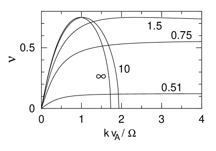
Figure 1: The growth rate of the Balbus-Hawley instability as a function of wavenumber for different choices of the Hall and Pedersen conductivities $\sigma_{1}$ and $\sigma_{2}$ (see text). Upper: the ambipolar or Ohmic diffusion limits ($\sigma_{1}=0$); middle: the Hall limit ($\sigma_{2}=0$) with $\sigma_{1}B_{z}>0$; and lower: the Hall limit for $\sigma_{1}B_{z}<0$. The curves in each panel are labelled by $\chi$, the ratio of the coupling frequency to the disc angular frequency: ideal MHD is recovered for $\chi\rightarrow\infty$, and the magnetic field is poorly coupled to the disc for $\chi<1$. Note that the scale on the horizontal axis differs between the lower and upper two plots – the ideal MHD curve labelled “$\infty$” appears in each plot.

4.3 Hall limit ($\sigma_{2}=0$) with $\sigma_{1}B_{z}>0$

The departure from the ideal limit changes markedly when the Hall term is introduced. In the absence of ambipolar diffusion, with $\sigma_{1}B_{z}>0$, one finds growth for wavenumbers between 0 and

$$k_{c}v_{A}/\Omega=\sqrt{3}\left(1+2\chi^{-1}\right)^{-1/2}\,,$$ (28)

and a maximum growth rate unchanged from the ideal limit, i.e. $\nu_{0}=\frac{3}{4}\,$! The corresponding wave number, however, decreases as the geometric mean of $\Omega$ and $\omega_{c}$ as $\chi\rightarrow 0$:

$$k_{0}v_{A}/\Omega=\sqrt{{\textstyle\frac{15}{16}}}\left(1+{\textstyle\frac{5}{4}}\chi^{-1}\right)^{-1/2}\,.$$ (29)

This behaviour is demonstrated in the middle panel of Fig. 1.

4.4 Hall limit ($\sigma_{2}=0$) with $\sigma_{1}B_{z}<0$

If the other Hall-dominated limit is taken, the behaviour is again different (see lower panel of Fig. 1). For $\chi>2$, the range of wave numbers for which growth occurs is finite, with

$$k_{c}v_{A}/\Omega=\sqrt{3}\left(1-2\chi^{-1}\right)^{-1/2}\,.$$ (30)

$k_{c}$ becomes infinite once $\chi$ reaches 2, and for $\frac{1}{2}<\chi<2$, all wave numbers grow. There is a fastest-growing mode for $\chi>\frac{5}{4}$, with $\nu_{0}=\frac{3}{4}$ and

$$k_{0}v_{A}/\Omega=\sqrt{{\textstyle\frac{15}{16}}}\left(1-{\textstyle\frac{5}{4}}\chi^{-1}\right)^{-1/2}$$ (31)

(cf. the $\chi=1.5$ case in the lower panel of Fig. 1). Again, this becomes infinite for $\chi=\frac{5}{4}$ For $\frac{1}{2}<\chi<\frac{5}{4}$, the growth rate is a monotonically increasing function of $k$, asymptotically approaching

$$\nu_{0}=(\chi-{\textstyle\frac{1}{2}})^{1/2}(2-\chi)^{1/2}$$ (32)

This limit decreases to zero for $\chi=\frac{1}{2}$ (cf. the $\chi=0.75$ and 0.51 curves in the lower panel of Fig. 1), at which point there are no longer any growing modes.

4.5 The general case

When $\sigma_{1}B_{z}>0$, there are growing modes with wave numbers between 0 and

$$k_{c}v_{A}/\Omega=\left(\frac{3\chi(\chi+{\textstyle\frac{1}{2}}s\sigma_{1}\sigma_{\perp}^{-1})}{\chi^{2}+{\textstyle\frac{5}{2}}\chi s\sigma_{1}\sigma_{\perp}^{-1}+1}\right)^{1/2}.$$ (33)

The maximum growth rate satisfies

$$\left(\frac{12\sigma_{2}\sigma_{\perp}^{-1}\,\nu_{0}}{9-16\nu_{0}^{2}}-{\textstyle\frac{1}{2}}s\sigma_{1}\sigma_{\perp}^{-1}\right)(1+\nu_{0}^{2})=\chi\,.$$ (34)

Figure 2: As for Fig. 1, but for intermediate cases. Upper panel: $\sigma_{1}B_{z}>0$ and $|\sigma_{1}|=\sigma_{2}$; middle panel: $\sigma_{1}B_{z}<0$ and $|\sigma_{1}|=\sigma_{2}$; and lower panel: $\sigma_{1}B_{z}<0$ with $|\sigma_{1}|=6\sigma_{2}$.

This behavior is illustrated in the top panel of Fig. 2, which shows the wave number dependence of the growth rate when $|\sigma_{1}|=\sigma_{2}$. As $\chi$ is reduced, the maximum growth rate and associated wave number decrease. However, in the limit $\chi\rightarrow 0$, the growth rate remains finite, with

$$\nu_{0}\approx\frac{3}{4}\,\frac{|\sigma_{1}|}{\sigma_{\perp}+\sigma_{2}}\,\,.$$ (35)

The corresponding wave number, however, decreases:

$$k_{0}v_{A}/\Omega\approx\left(\frac{3\chi}{4}\frac{|\sigma_{1}|}{\sigma_{\perp}+\sigma_{2}}\right)^{1/2}.$$ (36)

When $\sigma_{1}B_{z}<0$, growing modes exist only for $\chi>{\textstyle\frac{1}{2}}|\sigma_{1}|/\sigma_{\perp}$. If $|\sigma_{1}|/\sigma_{\perp}>\frac{4}{5}$, then eqs (33) and (34) hold; otherwise there is a restricted range of $\chi$ for which all wave numbers grow, determined by the inequality

$$\left(\chi-\frac{5|\sigma_{1}|}{4\sigma_{\perp}}\right)^{2}<\left(\frac{5|\sigma_{1}|}{4\sigma_{\perp}}\right)^{2}-1\,.$$ (37)

The middle panel of Fig. 2, shows the behaviour as $\chi$ is reduced for $|\sigma_{1}|=\sigma_{2}$. In this case the range of growing modes is always finite. The lower panel, for $|\sigma_{1}|=6\sigma_{2}$ demonstrates the existence of a small range of $\chi$ around 0.75 over which all wave numbers grow.

Figure 3: Maximum growth rate (in units of the Keplerian frequency $\Omega$) as a function of degree of coupling between the magnetic field and neutral gas, $\chi$, for different choices of the Hall and Pederson conductivities $\sigma_{1}$ and $\sigma_{2}$. Dotted curve: the ambipolar and Ohmic diffusion limits ($\sigma_{1}=0$); solid: the Hall limit ($\sigma_{2}=0$); dashed: the case $|\sigma_{1}|=\sigma_{2}$. The upper and lower members of the pairs of dashed or solid curves correspond to $\sigma_{1}B_{z}>0$ or $\sigma_{1}B_{z}<0$ respectively.

These results are summarised in Figures 3 and 4. Fig. 3 shows the maximum growth rate as a function of $\chi$ for different choices of $\sigma_{1}$ and $\sigma_{2}$. In the ambipolar and Ohmic diffusion limits ($\sigma_{1}=0$), the maximum growth rate decreases to zero as $\chi\rightarrow 0$. When the Hall term is included, the growth rate drops to zero at $\chi={\textstyle\frac{1}{2}}|\sigma_{1}|/\sigma_{\perp}$ for $\sigma_{1}B_{z}<0$, or remains finite at $\frac{3}{4}|\sigma_{1}|/(\sigma_{\perp}+\sigma_{2})$ for $\sigma_{1}B_{z}>0$.

Figure 4: A polar plot of the maximum growth rate of the Balbus-Hawley instability. The Cartesian cordinates of a point on the plane corresponds to $(\mathrm{sign}(B_{z})\sigma_{1},\sigma_{2})$ suitably normalised. The polar radius is $\chi$, the parameter controlling the degree of magnetic coupling in the disc. The contours are labelled by the maximum growth rate in units of $\Omega^{-1}$.

This behaviour is displayed more fully in Fig. 4, which shows contours of fixed growth rate in a polar plot. The ambipolar and Ohmic diffusion limits apply along the locus $\sigma_{1}=0$ running vertically through the origin. It is clear that the growth rate in the weak coupling limit ($\chi\la 1$) is sensitive to the form of the conductivity tensor, and that the behaviour in the two diffusion limits is not generally representative.

5 A two-fluid model for the Hall limit

It is surprising at first glance that the Hall conductivity allows the Balbus-Hawley instability to grow at a rate of order $\Omega$ in the formal limit of zero coupling. Here I address the physical explanation for this result, for simplicity focussing on the “pure” Hall case ($\sigma_{2}=0$). In the ambipolar diffusion limit, intuition is aided by a model two-fluid system: an ionized (but electrically-neutral) fluid into which the magnetic field is frozen; and a neutral fluid which is indirectly coupled to the magnetic field via collisions of the charged speicies with the neutrals. There is an analogous model in the Hall limit $|\sigma_{1}|\gg\sigma_{2}$.

In this model, the ionized component of the fluid can be regarded as consisting of two species, one of which does not suffer significant collisions with the neutrals, the other being so strongly tied to the neutrals by collisions that its drift velocity is negligible. For convenience, I shall refer to the former as “electrons” (subscript $e$) the latter as “ions” (subscript $i$); although the roles of these species could be played by other species, e.g. ions and grains, under suitable conditions.

The Hall parameters of the two species satisfy $|\beta_{i}|\ll 1\ll|\beta_{e}|$. Because the ions are strongly tied to the neutrals by collisions and are responsible for transmitting the electromagnetic stresses to the fluid, one may regard the ions and neutrals as a single fluid with the charge density of the ions and the inertia (and thermal pressure, when relevant) of the neutrals. This fluid is permeated by the electrons, into which the magnetic field is frozen.

In this limit the components of the conductivity perpendicular to the magnetic field are

$$\sigma_{1}\approx\frac{ecn_{i}Z_{i}}{B}$$ (38)

and

$$\sigma_{2}\approx\left(|\beta_{i}|+|\beta_{e}|^{-1}\right)|\sigma_{1}|$$ (39)

(where I have used $n_{i}Z_{i}=-n_{e}Z_{e}$ in eq. 38). The current is dominated by the electrons, which drift perpendicular to the magnetic and electric field so that the net Lorentz force on them is zero – collisions with the neutrals play a negligible role in their equation of motion. The drift of the ions with respect to the neutrals, however, is strongly inhibited by collisions, and is determined by the balance between the electric field and the drag associated with the neutrals. Thus

$$\mn@boldsymbol{J}\approx n_{e}Z_{e}e\mn@boldsymbol{v}_{e}\approx\sigma_{1}\mn@boldsymbol{\hat{B}}\mn@boldsymbol{\times}\mn@boldsymbol{E^{\prime}_{\perp}}\,.$$ (40)

The electromagnetic stresses on the fluid are communicated largely by the collisions with the ions:

$$\frac{\mn@boldsymbol{J}\mn@boldsymbol{\times}\mn@boldsymbol{B}}{c}\approx\sigma_{1}\mn@boldsymbol{E^{\prime}_{\perp}}\approx\gamma_{i}\rho\rho_{i}\mn@boldsymbol{v}_{i}$$ (41)

Because the ion-neutral drift speed $\mn@boldsymbol{v}_{i}$ is small, the associated dissipation is small: $\mn@boldsymbol{J}\cdot\mn@boldsymbol{E^{\prime}_{\perp}}\approx\sigma_{2}E_{\perp}^{\prime 2}$, tending to zero in the limit $\sigma_{2}\rightarrow 0$. With this model fluid, one can use the linearized equations (13)–(16) to understand the growth of the instability in the Hall limit as $\chi\rightarrow 0$.

First consider the wave modes supported by the fluid in the absence of rotation. At small wavenumbers (long wavelengths) the fluid supports the Alfvén waves of ideal MHD, while at wavenumbers far in excess of $\omega_{c}/v_{A}$, there are two circularly-polarized modes (Wardle & Ng 1999). In one, the electrons and magnetic field are relatively unperturbed, and the ion-neutral fluid executes gyrations about the field direction at the frequency $\omega\approx\omega_{c}$. In the other, the ion-neutral fluid is static and the electrons and magnetic field twist about the unperturbed field direction with the opposite sense of rotation. The frequency of this mode scales quadratically with wavenumber, as the diffusive term $\nabla\mn@boldsymbol{\times}\mn@boldsymbol{E}^{\prime}$ dominates $\nabla\mn@boldsymbol{\times}(\mn@boldsymbol{v}\mn@boldsymbol{\times}\mn@boldsymbol{B})$ in the induction equation: $\omega\approx(kv_{A})^{2}/\omega_{c}$. The sense of rotation of either mode is determined by the sign of $\sigma_{1}B_{z}$.

Finally, consider the effect of rotation, which attempts to enforce epicyclic motion of the ions and neutrals with frequency $\Omega$ through the Coriolis and angular terms in the momentum equation. For $\chi\ll 1$, $\Omega\gg\omega_{c}$, so the rotation can only couple effectively to the second mode for wave numbers $kv_{A}\approx\sqrt{\omega_{c}\Omega}$. The generation of toroidal field from poloidal field by the shear in the disc (see eq. 4) acts as a forcing term for this circularly polarized mode, which grows or decays depending on whether the shear assists or opposes the rotation of the magnetic field, i.e. depending on the sign of $\sigma_{1}B_{z}$.

6 Discussion

The Hall conductivity modifies the growth of the Balbus-Hawley instability in weakly ionized discs when the magnetic field is not well-coupled to the neutral matter. The effect depends on the relative signs of $\sigma_{1}$ and the initially vertical field $B_{z}$. For $\sigma_{1}B_{z}>0$ the growth rate remains of order the Keplerian frequency $\Omega$ as the coupling is reduced, and the wavelength of the fastest growing mode scales as $\chi^{1/2}$. On the other hand, if $\sigma_{1}B_{z}<0$, the mode is damped for $\chi\la{\textstyle\frac{1}{2}}$. The dependence on the initial field being parallel or antiparallel to the disc rotation axis arises ultimately from the intrinsic handedness introduced into the medium by the difference in the drifts of positive and negative species. In the limit $\Omega\rightarrow 0$, the unstable mode corresponds to a standing, circularly-polarized Alfvén wave; left and right-circularly polarized Alfvén waves propagate differently according to the sign of $\sigma_{1}B_{z}$ (Wardle & Ng 1999).

This is to be contrasted with the ambipolar and Ohmic diffusion limits (Blaes & Balbus 1994; Jin 1996), where the growth rate is independent of the sign of $B_{z}$, declining steadily while the wavelength increases linearly as the coupling parameter is reduced. Blaes and Balbus found that the growth rate increases again for $\chi\la\rho_{i}/\rho$, when the coupling becomes so poor that the momentum-exchange time scale for the ions with the neutrals, $(\gamma_{i}\rho)^{-1}$ is longer than the Keplerian time scale $\Omega^{-1}$. Then the instability develops in the ionized component and magnetic field without affecting the neutrals. This behaviour does not occur here because I neglected the inertia of the charged species (see Section ) – the formulation in Section 2 is valid only for frequencies well below $\gamma_{i}\rho$, and thus implicitly assumes that $\Omega\ll\gamma_{i}\rho$, i.e. $\chi\gg\rho_{i}/\rho$. The ionization fraction in protostellar discs is so low that this approximation is very good indeed, and if the coupling were this poor any dynamically important magnetic field would remove itself (and the ions) from the disc on the Alfvén crossing time in the ionized fluid. The ionized species cannot, therefore, decouple from the neutrals in any practical sense.

For a favourable alignment between the magnetic field and rotation axis (i.e. $\sigma_{1}B_{z}>0$), the growth rate in the weak-coupling limit remains within a factor of a few of $\Omega$. The practical limit on the coupling is determined by the wavelength as the coupling gets weak, as this must be less than the scale height $h$ of the disc. If $c_{s}$ is the isothermal sound speed, so that $h=c_{s}/\Omega$, the wavelength of the fastest-growing mode becomes of order $h$ when the coupling parameter $\chi$ reaches $v_{A}^{2}/c_{s}^{2}$. The corresponding limit in the ambipolar diffusion case is $v_{A}/c_{s}$ which would produce a growth rate of order $(v_{A}/c_{s})\Omega$.

A study of the nonlinear development of the instability requires a numerical simulation. For now, I note that the strength of the magnetic field affects the conductivity through the Hall parameters, with a larger field increasing the degree of flux-freezing in the ionized component. Thus there is the possibility of the instability beginning in the Hall regime, with the field strength growing to the point that the fluid enters the ambipolar diffusion regime.

These results are applicable to protostellar discs, where collisions are sufficient to decouple ions and grains from the magnetic field (Wardle & Königl 1993). Indeed, the Hall conductivity is of the same order as the ambipolar diffusion term over a broad range of parameters (Wardle & Ng 1999). Further the coupling parameter is thought to be small near the midplane in protostellar discs, particularly at radii around one AU where the temperature is low enough that thermal ionization is not yet effective, and the surface density is high enough to shield the material from cosmic rays (Hayashi 1981; Gammie 1996; Wardle 1997). The magnitude and relative size of the components of the conductivity tensor vary strongly with height in the disc as the neutral density decreases near the disc surface, and the ionization level increases because of exposure to cosmic rays (Gammie 1996; Wardle 1997) and X-rays from the central star (Glassgold et al 1997). In particular, although the instability is not very efficient in transporting angular momentum when the coupling is weak, the column density within this portion of the disc is relatively large, so that the net angular momentum transport can be comparable to that in the layers closer to the surface.

The dependence on the sign of the initial field raises the intriguing possibility that the accretion process, and the formation of magnetically-driven disc winds are dependent on the sign of the magnetic field. This issue is linked to the collapse of cloud cores to form protostars and discs, which presumably brings in some fraction of the interstellar field to be the initial disc field. While the calculations of core collapse to date are instructive (e.g. Fiedler & Mouschovias 1993; Basu 1997; Contopoulos, Ciolek, & Konigl 1998; Li 1998; Ciolek & Königl 1998), none include the Hall effects, which are also important during this phase (Wardle & Ng 1999). Angular momentum transport during collapse will also depend on whether the field is parallel or antiparallel to the core’s angular momentum vector, and one might imagine that this leads to a preferential orientation within discs, but this is unclear as the sign of $\sigma_{1}$ may change between the collapse and disc phases as grains, then ions become successively decoupled from the magnetic field with increasing neutral density.

7 Summary

This paper examined the Balbus Hawley instability of a vertical magnetic field in a weakly-ionized, thin Keplerian disc. The vertical stratification was ignored, and radial and azimuthal variations were neglected. The resulting linearized equations are valid for wavelengths small compared to the disc scale height. I examined the dispersion relation. The conductivity tensor contributes two parameters: (i) a coupling parameter $\chi$, the ratio of the frequency at which the finite conductivity becomes important to the Keplerian angular frequency; and (ii) the ratio $\mathrm{sign}(B_{z})\sigma_{1}/\sigma_{\perp}$, which reflects the contributions of the Hall and Pedersen conductivities, $\sigma_{1}$, $\sigma_{2}$ respectively, to the total conductivity perpendicular to the magnetic field $\sigma_{\perp}=(\sigma_{1}^{2}+\sigma_{2}^{2})^{1/2}$.

I found the following:

1. The Hall conductivity substantively modifies the behaviour of the instability once finite conductivity effects become important ($\chi\la 1)$. If the rotation axis of the disc defines the $z$ direction, the departure from the ambipolar diffusion limit depends on the sign of $\sigma_{1}B_{z}$.

2. For $\sigma_{1}B_{z}>0$, growth occurs over a finite range of wavenumbers. For poor coupling ($\chi\ll 1$), the maximum growth rate remains finite, tending to a value $\frac{3}{4}|\sigma_{1}|/(\sigma_{\perp}+\sigma_{2})\,\Omega$ while the associated wave number scales as $\sqrt{\chi}$. This should be contrasted with the ambipolar diffusion case (Blaes & Balbus 1994) for which the growth rate and wave number scale linearly in $\chi$.

3. For $\sigma_{1}B_{z}<0$, on the other hand, there is no instability when the coupling is poor: growth requires $\chi>{\textstyle\frac{1}{2}}|\sigma_{1}|/\sigma_{\perp}$. There is generally a limited range of wave numbers, over which growth occurs. However, if $|\sigma_{1}|/\sigma_{\perp}<\frac{4}{5}$, there is a limited range of $\chi$ around the value $|\sigma_{1}|/\sigma_{\perp}$ for which all wave numbers grow.

4. Although the instability has a formal growth rate of order $\Omega$ in the limit of zero coupling when $\sigma_{1}B_{z}>0$, the wavelength is limited by the disc scale height, and therefore growth will only occur for $\chi\ga v_{A}^{2}/c_{s}^{2}$. Note that this constraint is far less severe than in the ambipolar diffusion limit, which requires $\chi\ga v_{A}/c_{s}$.

Finally, I stress that these results indicate the qualitative changes to dynamical behaviour to be expected when ambipolar diffusion breaks down during the collapse of cloud cores to form protostars and during the subsequent evolution of their attendant discs.

I thank Charles Gammie and the referee for comments on the manuscript. The Special Research Centre for Theoretical Astrophysics is funded under the Special Research Centres programme of the Australian Research Council.

References

- [] Balbus, S. A. & Hawley, J. F. 1991, ApJ, 376, 214
- [] Basu, S. 1997, ApJ, 485, 240
- [] Blaes, O. M. & Balbus, S. A. 1994, ApJ, 421, 163
- [] Chandrasekhar, S. 1961, Hydrodynamic and hydromagnetic stability (Oxford: Oxford University Press)
- [] Ciolek, G. E. & Konigl, A. 1998, ApJ, 504, 257
- [] Contopoulos, I., Ciolek, G. E. & Konigl, A. 1998, ApJ, 504, 247
- [] Cowling, T. G. 1957, Magnetohydrodynamics (New York: Interscience)
- [] Fiedler, R. A. & Mouschovias, T. C. 1993, ApJ, 415, 680
- [] Gammie, C. F. 1996, ApJ, 457, 355
- [] Glassgold, A. E., Najita, J. & Igea, J. 1997, ApJ, 480, 344
- [] Hawley, J. F. & Balbus, S. A. 1991, ApJ, 376, 223
- [] Hawley, J. F. & Stone, J. M. 1998, ApJ, 501, 758
- [] Hayashi, C. 1981, Prog Theor Phys Supp, 70, 35
- [] Jin, L. 1996, ApJ, 457, 798
- [] Li, Z.-Y. 1998, ApJ, 493, 230
- [] MacLow, M.-M., Norman, M. L., Königl, A. & Wardle, M. 1995, ApJ, 442, 726
- [] Nakano, T. & Umebayashi, T. 1986, MNRAS, 218, 663
- [] Nishi, R., Nakano, T., Umebayashi, T. 1991, ApJ, 368, 181
- [] Norman, C. & Heyvaerts, J. 1985, AA, 147, 247
- [] Pilipp, W., Hartquist, T. W., Havnes, O. & Morfill, G. E. 1987, ApJ, 314, 341
- [] Sano, T., Inutsuka, S.-I. & Miyama, S. M. 1998, ApJ, 506, L57
- [] Stone, J. M., Hawley, J. F., Gammie, C. F. & Balbus, S. A. 1996, ApJ, 463, 656
- [] Tout, C. A. & Pringle, J. E. 1992, MNRAS, 259, 604
- [] Velikhov, E. P. 1959, JETP, 36, 1398
- [] Wardle, M. & Königl, A. 1993, ApJ, 410, 218
- [] Wardle, M. 1997, in Proc. IAU Colloq. 163, Accretion Phenomena and Related Outflows, ed. D. Wickramasinghe, L. Ferrario & G. Bicknell (San Francisco: ASP), 561
- [] Wardle, M. & Ng, C. 1999, MNRAS, 303, 239