2 $\mu$m Narrow–Band Imaging of the Sagittarius D H II Region

Abstract

We present 2 $\mu$m narrow–band images of the core H II region in the Galactic star forming region Sagittarius D. The emission–line images are centered on 2.17 $\mu$m (Br$\gamma$) and 2.06 $\mu$m (He I). The H II region appears at the edge of a well defined dark cloud, and the morphology suggests a blister geometry as pointed out in earlier radio continuum work. There is a deficit of stars in general in front of the associated dark cloud indicating the H II region is located in-between the Galactic center and the sun. The lesser spatial extent of the He I line emission relative to Br$\gamma$ places the effective temperature of the ionizing radiation field below 40,000 K. The He I 2.06 $\mu$m to Br$\gamma$ ratio and Br$\gamma$ / far infrared dust emission put $T_{\rm eff}$ at about 36,500 K to 40,000 K as derived from ionization models.

1 INTRODUCTION

Sagittarius D (Sgr D) is a well known star forming region seen toward the Galactic center (GC). The associated H II region (compact plus extended components) was noted in the survey of Downes et al. (1978). To be clear, the subject of this paper is the compact H II region (see the maps of Lizst 1992) which is superimposed on a much larger, extended or diffuse H II region. These are very close to the prominent super nova remnant (SNR) known as the Sgr D SNR. We will call the compact Sgr D H II region “H II region” or “Sgr D H II region.” We will call the larger region the “extended H II region.” Sgr D has been observed at radio continuum wavelengths (Odenwald 1989; Lizst 1992; Mehringer et al. 1998), in radio recombination lines (RRL, Whiteoak & Gardner 1974, Anantharamaiah & Yusef–Zadeh 1989), in CS and H₂CO lines (Kázes & Aubry 1973; Whiteoak & Gardner 1974, Lis 1991; Mehringer et al.1998), and in the far infrared (Odenwald & Fazio 1984 ).

The location, and therefore the total luminosity and mass associated with Sgr D, is uncertain. Lis (1991) pointed out that the line widths of the CS emission lines he associated with the H II region are narrow and therefore not likely to arise from a giant molecular cloud (GMC) in the GC nuclear disk as had been previously thought. The line widths in the GC nuclear disk GMCs are typically much larger than those observed toward Sgr D or in the GMCs of the Galactic disk. Lis (1991) suggested that Sgr D could be either in the foreground ($\sim$ 3.5 kpc) or part of the expanding molecular ring, a complex located within a few hundred parsec of the GC. Mehringer et al. (1998) favor an in–or–beyond the GC distance for Sgr D (see the discussion below).

The present images were obtained as part of an ongoing narrow–band survey of the inner Galaxy designed to find emission–line stars. The 2 $\mu$m images provide the most detailed spatial and morphology information to–date on the compact Sgr D H II region and can be used to infer information regarding the line of sight position of the Sgr D H II region and to constrain the properties of the stellar source(s) responsible for the ionization.

2 OBSERVATIONS AND DATA REDUCTION

The narrow–band images were obtained on the nights 27 and 28 July 1996 using the Cerro Tololo Interamerican Observatory (CTIO) facility infrared imager CIRIM on the 1.5–m telescope (f/8). CIRIM employs a NICMOS III array and is fully described in the CIRIM instrument manual available from CTIO (http://www.ctio.noao.edu).

The images of Sgr D were obtained as part of a narrow–band survey of the inner Galaxy designed to detect emission–line stars (Blum & Damineli 1999) . The narrow–band line filters employed for this survey are 2.06 $\mu$m (He I, hereafter the 206 filter, $\sim$ 0.5 $\%$), 2.08 $\mu$m (C IV, 208, $\sim$ 0.5$~{}\%$), and 2.17 $\mu$m (Br$\gamma$, 217, $\sim$ 1 $\%$). Continuum filters are also used so that line fluxes can be measured; however, due to large and non–uniform interstellar reddening, continuum filters are employed on each side of the lines to more accurately determine the continuum at the line position. The continuum filters are 2.03 $\mu$m (203, $\sim$ 0.5 $\%$), 2.14 $\mu$m (214, $\sim$ 0.5 $\%$), and 2.248 $\mu$m (225, $\sim$ 1 $\%$). The bandwidths are rough estimates from transmission scans provided by the manufacturers, Omega Optical (203, 206, 208, 214) and Barr Assoc. (217, 225). The 206 filter is slightly more peaked than the 217 filter. We estimate that the 206 line fluxes will have an uncertainty $\mathrel{\hbox{\hbox to0.0pt{\hbox{\lower 4.0pt\hbox{$\sim$}}\hss}\hbox{$<$}}}$ 10 $\%$ due to transmission profile.

The 208 filter is designed to detect ionized carbon (C IV) in emission–line stars and is essentially another continuum filter for purposes of investigating H II regions. The 225 filter is a molecular hydrogen filter, but is used as a continuum point for the emission–line star survey where such emission is expected to be absent. In the present case, there could be some H₂ emission contributing to the 225 filter, but we expect it to be small relative to H II region emission as is the case, for example, in the Orion nebula (Bautista et al. 1995). Furthermore, any contribution by H₂ is mitigated by the fact that we use a linear fit to the four continuum points (203, 208, 214, 225) to determine the continuum at the emission–line positions. The derived continuum at 2.248 $\mu$m is $\mathrel{\hbox{\hbox to0.0pt{\hbox{\lower 4.0pt\hbox{$\sim$}}\hss}\hbox{$<$}}}$ 10 $\%$ higher than the derived continuum at 2.06 $\mu$m for 5^′′ to 55^′′ radius apertures centered on the H II region.

The plate scale of CIRIM at f/8 is approximately 1.16^′′ pix^-1, 1.17^′′ pix^-1, 1.18^′′ pix^-1, 1.18^′′ pix^-1, 1.19^′′ pix^-1, and 1.19^′′ pix^-1 for the 225, 217, 214, 208, 206, and 203 filters, respectively. The images were taken in strips one degree long in right ascension (and one frame high, or five arcmin in declination), each image offset by 99^′′ from the previous. The strips were obtained by stepping the telescope in one direction for one full degree, then stepping back in the reverse direction in the next filter. When a complete strip was completed in all filters, an offset north was made and a new strip begun. The northern offset was made with an eastern one to keep the survey area centered along the Galactic plane. A total of nearly three square degrees has been observed to date.

Individual images had exposure times of 5 seconds in the 225 and 217 filters and 15 seconds for the remaining four filters. The seeing on individual frames was about 1.9^′′ to 2.0^′′ (measured FWHM). This image quality was degraded by $\sim$ $5-6\%$ after combining the images (see below).

All basic data reduction was accomplished using IRAF. Each image was flat–fielded using dome flats and then sky subtracted using a median combined image of approximately 35 data frames. A set of seven sky subtracted frames covering the area around the H II region (in each filter) was combined to form a final image in each filter. Each of these six final images was then trimmed on either end such that it comprised an area everywhere sampled by three individual frames and was roughly centered on the H II region. This trimming of the ends of the combined images resulted in a final area of $\sim$ 8.1${}^{\prime}\times 5.0^{\prime}$ for each image. No pixel shifts were made or trimming done in the declination direction to obtain the final images.

Each narrow–band image was flux calibrated using the the Elias et al. (1982) standard HD 161743 (B9). This star was observed three times during the night of 27 July over a range in airmass bracketing the observations. Only the 214 filter was observed on 28 July and the standard star observations were obtained at an airmass within a few percent of the Sgr D 214 data. The standard deviation in the mean of the standard star measurements was less than one percent for each of the six filters. We adopt the least square fit uncertainty for each filter as a function of airmass as the uncertainty for the flux calibration (except for 214). This was less than five percent in all cases and typically a few percent. The flux for each filter was set by the ratio of the 2.2 $\mu$m flux to the flux at the filter wavelength as determined from a blackbody with $T_{\rm eff}$ of 10,600 K, appropriate for a B9 V (Johnson 1966).

HD 161743 is a B9 IV star and thus has intrinsic Br$\gamma$ absorption. We have made a small correction (0.10 mag) to the 217 magnitudes to account for this. Measurements of the G5 V star HD 1274 (Carter & Meadows 1995; transformed to the CTIO/CIT system, Carter 1990) suggest an 0.05 mag difference in the Br$\gamma$ absorption relative to HD 161743. The Ali et al. (1995) and Hanson, Conti, & Rieke (1996) spectroscopic observations of B and G stars suggest G5 V stars have non-negligible Br$\gamma$, about half that expected for a B9 IV star, hence the correction of 0.10 mag.

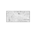
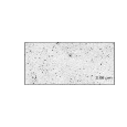
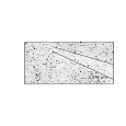
Figure 1: Narrow–band images. North is up and East to the left. The scale is 1.2^′′ pix^-1 and each image covers roughly 8^′ $\times$ 5^′. The images are 2.17 $\mu$m (Br$\gamma$ $+$ continuum), 2.06 $\mu$m (He I $+$ continuum), and 2.248 $\mu$m continuum from top to bottom respectively. The lack of stars in projection against the dark cloud (indicated by by the lines in the 2.248 $\mu$m image), suggests it is relatively in the foreground; see text. Not shown are the 203, 208, and 214 images. Continuum subtracted images are shown in Figure 2.

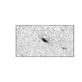
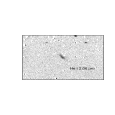
Figure 2: Continuum subtracted line images. North is up and East to the left. Each image covers roughly 3.5^′ $\times$ 2.5^′ centered on the H II region. The images are Br$\gamma$ (217$-$225; see text), and He I 2.06 $\mu$m (206$-$214). The sharp edge to the Br$\gamma$ and He I 2.06 $\mu$m emission toward the dark cloud indicates that the H II region is physically associated with it. The appearance and measured extent of the Br$\gamma$ emission is larger than that for the He I emission; this is confirmed in Figure 5.

Aperture photometry was computed in all six filters centered on the compact H II region using the IRAF “PHOT” package. The Br$\gamma$ peak defines the aperture center on all images. This peak is the same in Figure 1b and Figure 2a to about 1 pixel. A correction was made to the background by specifying a background aperture located on the darkest area of the cloud about one arcminute to the SW from the edge of the H II region. This background eliminates incomplete sky subtraction resulting from differences in the combined image sky frame and the subset of images for the H II region, as well as a low level background due to the extended H II region. The largest residual sky was three percent for the 217 image. Of course, nonuniform emission from the extended H II region will not be accounted for.

In addition to aperture photometry, DoPHOT (Schecter, Mateo, & Saha 1993) point–spread–function (psf) fitting photometry was obtained for point sources in the field. Version 3.0 of the code was used. The point source photometry is primarily for use in the search for emission–line stars but is useful in the present case to estimate interstellar reddening to stars near the H II region. For the psf fitting photometry, an additional aperture correction was determined for each image to transform the DoPHOT magnitudes to the standard star magnitudes. This was accomplished by measuring aperture magnitudes for 10–15 stars on each image. The corrections obtained in this way had standard deviations in the mean of two to four percent.

3 RESULTS AND DISCUSSION

The narrow–band images in the 206, 217, and 225 filters are shown in Figure 1; the 203, 208, and 214 filter images are not shown. The compact H II Region is the obvious feature toward the center–north of these images. Continuum subtracted line images are shown in Figure 2. The continuum subtracted images use the 225 and 214 images for the Br$\gamma$ and He I 2.06 $\mu$m continuum, respectively. The extent in the Br$\gamma$ image (Figure 2) is roughly 21.5^′′ $\times$ 8.5^′′ FWHM, compared to the 25^′′ $\times$ 10^′′ in the 1616 MHz VLA maps reported by Liszt (1992) and 20^′′ $\times$ 10^′′ reported by Mehringer et al. (1998). Mehringer et al. (1998) analized the 1616 MHz (18 cm) data of Liszt (1992) and also new 6 cm data. The measured FWHM of the He I image (Figure 2) is 18.8^′′ $\times$ 6.3^′′. We verified the source position by matching point sources from a visual image centered on the radio position of Liszt (1992, source 3, $\alpha_{1950},\delta_{1950}=$ 17^h 45^m 32^s.1, $-$28^∘ 00^′ 43^′′) to the infrared sources on our images. The visual image was obtained from the digitized sky survey (DSS). No indication of the H II region appears on the DSS image.

3.1 Image Morphology and Reddening to the H II Region

The morphology of the H II region appears to be one of a blister on the edge of a clearly delineated dark cloud as pointed out by Odenwald (1989) from radio continuum images. The very sharp edge to the line emission toward the cloud leaves little doubt that the cloud and H II region are physically related. Figure 3 shows contour plots of the 225 (2.248 $\mu$m continuum) filter and Br$\gamma$ filter images. The H II region is much less extended in the continuum, and there is a strong suggestion of three embedded sources at the location of the peak Br$\gamma$ emission. None of these appears truly point–like but this may be largely due to their close proximity to one another and the contamination by extended emission. Alternately, each peak may be a group of embedded stars or perhaps a knot of gas.

In stark contrast to the obvious dark cloud is the crowded stellar field, well known at 2 $\mu$m toward the GC. The lack of stars in projection against the cloud strongly suggests it is more or less in the foreground. Indeed, the stellar density peaks so dramatically toward the inner Galaxy (see Kent 1992 and references therein) that it is difficult to construct a plausible model which does not place the dark cloud between the sun and the GC.

3.1.1 Interstellar Extinction to Individual Stars

We have determined $A_{K}$ for individual stars with measurements in all six narrow–band filters by fitting to three model flux distributions, a 10,000 K blackbody, a 5,000 K blackbody, and a bulge late M giant (none of these stars had narrow–band indices suggesting an emission–line object). The latter model was constructed from spectra of bulge M giants (Terndrup, Frogel, & Whitford 1991) as tabulated by Blum, Sellgren, & DePoy (1996$b$). The primary difference between models is the intrinsic absorption by H₂O in the late M giants toward the blue end of the $K-$band which mimics the effect of reddening. There is more curvature in the M giant spectra combined with reddening than for a reddened blackbody, and so the former model can improve the fit substantially for some stars. Our filters are all blueward of the CO bandhead at 2.3 $\mu$m which is prominent in M giants. A Mathis (1990) reddening law was adopted and $A_{K}$ values assigned to the individual stars based on the best fit among the three models (typically the spread in $A_{K}$ is about 1.5 mag for the 10,000 K and M giant models).

For 205 stars with six filter photometry, we find $A_{K}$ $=$ 2.3 $\pm$ 1.9 mag. Concentrating on the area around the H II region (to be quantitative we will consider a 3.5^′ $\times$ 2.5^′ area centered on the H II region with roughly equal area on and off the dark cloud), we find the majority of stars have $A_{K}$ $\leq$ 1.5 mag (18 of 34 stars with measured $A_{K}$ in this sub–region). Some stars were too faint or in crowded regions and thus did not have photometry in all filters. However, in this region, all but one of the stars seen in projection against the dark cloud can be accounted for either because they have a measured $A_{K}$ value, or because they appear on the DSS image. The one star with no DSS counterpart and no $A_{K}$ value is $\sim$ 1^′ away from the H II region. Another star which appears near the middle of the dark cloud has $A_{K}$ $=$ 5.5 mag. This may be an embedded object. Except for these two objects, the remainder of the stars seen in projection against the cloud have $A_{K}$ $\mathrel{\hbox{\hbox to0.0pt{\hbox{\lower 4.0pt\hbox{$\sim$}}\hss}\hbox{$<$}}}$ 1.5 mag or DSS counterparts. We have obtained estimates of the $V$ magnitudes for the latter (seven stars) from the DSS image and revised photometric calibration⁴ available from the Catalog and Surveys Branch on the Space Telescope Science Institute www pages. These stars have $V$ $\mathrel{\hbox{\hbox to0.0pt{\hbox{\lower 4.0pt\hbox{$\sim$}}\hss}\hbox{$>$}}}$ 15.5 mag. The majority are upper limits to the brightness because they are fainter than the faint limit of the non–linear calibration, but within 40 $\%$ of the counts of the faint end of the calibration ($V=$ 15.91 mag $\pm$ 0.5 mag). We derived estimates of the corresponding $K$ magnitudes for each of these stars from aperture photometry on the 225 image ($V-K$ from 1.8 to $\mathrel{\hbox{\hbox to0.0pt{\hbox{\lower 4.0pt\hbox{$\sim$}}\hss}\hbox{$>$}}}$ 3.8). All are consistent with late type (K or M) foreground dwarfs.

The closest star to the H II region ($\mathrel{\hbox{\hbox to0.0pt{\hbox{\lower 4.0pt\hbox{$\sim$}}\hss}\hbox{$<$}}}$ 8^′′) with no DSS counterpart has $A_{K}$ $=$ 1.0 mag (star “A” in Figure 3). This star had a best fit with the M giant model (reduced $\chi$ square $<$ 1). The 10,000 K blackbody model (reduced $\chi$ square = 1.5) gives $A_{K}$ $=$ 2.4 mag. Of course, off the dark cloud but within the near region, there are stars with larger $A_{K}$. This includes two located 10–15 arcsec north of the center of the H II region (stars “B” and “C” in Figure 3) with indicated $A_{K}$ $\sim$ 5 mag. Their proximity to the H II region suggests they may be young stellar objects with infrared excesses. Alternately, they may be background sources seen through the large column of material at the edge of the cloud.

3.1.2 Star Counts

Next, we considered star count models in order to compare the expected numbers of stars in the field relative to those in projection against the cloud with what is observed in the images. Our models have two extinction components, a uniform screen and the cloud itself. The uniform screen affects all stars in the field of view which lie behind it. The cloud can be thought of as a source of infinite extinction so that we see only foreground stars in front of it. This will be approximately true toward the center regions of the cloud and less so near the edges where background stars will be seen. In addition, embedded sources in the cloud could be projected upon the cloud at any location. Embedded sources should be quite reddened. Foreground stars projected against the cloud (or in the rest of the field) should be relatively blue. The position of the cloud along the line of sight will set (roughly) the relative numbers of stars in the cloud foreground compared to the background field. The H II region appears clearly related to the dark cloud; thus, any constraints on the location of the dark cloud should apply to the H II region.

We have detected stars in the narrow–band images down to $K\approx 14.5$ mag. A histogram of the 225 filter narrow–band magnitude ($K_{225}$, $\lambda$ $=$ 2.248 $\mu$m) is shown in Figure 4. There is a break at about $K_{225}$ $=$ 11 mag which suggests the completeness limit (likely set by crowding) is at this magnitude or brighter. We estimated the actual completeness limit by adding artificial stars to the $K_{225}$ image. Extracting stars from ten artificial images (with 300 artificial stars added to each), we find the $K_{225}$ counts are about 95 $\%$ complete to $K_{225}$ $=$ 11th magnitude, 87 $\%$ to 12th magnitude, and 77 $\%$ to 13th magnitude.

The cumulative counts in the 225 filter are 115 to $K_{225}$ $\leq$ 11 mag. The number with $K_{225}$ $\leq$ 11 mag and in projection against the dark cloud is seven for the darkest central strip which cuts from the north east to the south west on the frame (see Figure 1c). Accounting for an area of 18 $\%$ of the frame covered by this darkest region of the cloud, we find there are $\mathrel{\hbox{\hbox to0.0pt{\hbox{\lower 4.0pt\hbox{$\sim$}}\hss}\hbox{$<$}}}$ 29 $\%$ $\pm$ 10 $\%$ as many stars in the foreground of the dark cloud per unit area as there are in the remainder of the field (The uncertainty assumes Poisson statistics in the star counts.). We can use the models to estimate the distance where this would occur.

We have computed cumulative star count models as described by Blum et al. (1994). These models are based on the Kent (1992) two component bulge and disk model and assume the sun–to–GC distance is 8 kpc. The associated luminosity functions are for a broad band $K$ filter ($\lambda$ $=$ 2.2 $\mu$m). We will assume the 225 filter counts ($\lambda$ $=$ 2.248 $\mu$m) are equivalent to those in $K$.

A model with a uniform screen of extinction ($A_{K}=2.2$ mag at 4 kpc from the sun), matches the actual counts: 121 stars with $K$ $\leq$ 11 mag (correcting for 5 $\%$ incompleteness). This model is not too unreasonable given that the neutral hydrogen in the disk peaks rather strongly at this distance from the sun (for a sun–to–GC distance of 8 kpc, Burton 1988), and the average $A_{K}$ as determined from individual stars is 2.7 mag $\pm$ 2 mag (for stars with $K_{225}$ $\leq$ 11.0 mag). This $A_{K}$ value should be viewed with caution since only stars with measurements in all six filters were used (64 stars of the 115 with $K_{225}$ $\leq$ 11.0 mag). Still, it is in agreement with mean values to other fields toward the inner Galaxy (Catchpole, Whitelock, & Glass 1990; Blum, DePoy, & Sellgren 1996$a$ ).

If the dark cloud blocked all star light behind it and the 29 $\%$ of the stars we see are foreground (indeed, many of the infrared sources in projection against the cloud are seen in the DSS image), then the model would predict its distance at 6.0 kpc $\pm^{1.5}_{2.5}$ kpc. The screen of extinction may be placed variously between 2 and 6.2 kpc, and the extinction varied between 2.0 and 3.0 mag to still match the observed counts. For this range of parameter space, the cloud can be located between 3.9 and 7.9 kpc. It is possible to have models with the dark cloud quite close to the GC because the bulge stellar distribution is very peaked. Therefore, models with the screen nearer the sun will have fewer nearby disk stars, and so, to reach 29 $\%$ of the total requires the dark cloud to be closer to the GC. However, because the bulge distribution is so peaked, it cuts off very rapidly after the GC. For all the models (including a model with no extinction), even the point at which 50 $\%$ of the total counts (to $K$ $=$ 11 mag) are reached is always on the near side of the GC.

3.2 Recombination Lines

The integrated flux as a function of aperture radius is shown for the He I 2.06 $\mu$m line and Br$\gamma$ in Figure 5 where the center of the apertures was taken as the peak in the Br$\gamma$ image (Figure 2a). The line fluxes have been continuum subtracted. The continuum at the line center was taken from a linear least–squares fit to the 203, 208, 214, and 225 fluxes. Each curve reaches a point where the increase in flux between successive apertures changes sharply. For the He line, a clear maximum is reached near 15^′′. The apparent decrease in flux in He I 2.06 $\mu$m at larger radii may be due to a slight over–subtraction of the background. For Br$\gamma$, the slope change occurs at about 35^′′ where the total flux remains nearly constant. The possible increase at large radii may be due to non–uniform emission in the extended H II region. The He I and Br$\gamma$ radial extents are consistent with the FWHM values reported above; there is little additional flux beyond a radius of $\sim$ 20^′′–25^′′ (see Figure 5). As suggested by the appearance of the H II region in Figure 2, these results point to a smaller ionized volume of He than H. This, in turn, points to a relatively cool star(s) responsible for the ionizing radiation field (Osterbrock 1989).

According to Osterbrock (1989), equal volumes of ionized He and H do not occur until the effective temperature of the ionizing star is $T_{\rm eff}$$\mathrel{\hbox{\hbox to0.0pt{\hbox{\lower 4.0pt\hbox{$\sim$}}\hss}\hbox{$>$}}}$ 40,000 K. For spherical volumes and an ionization bounded H II region, Osterbrock (1989) has plotted the ratio of radii between the He and H volumes vs. $T_{\rm eff}$ (his Figure 2.5). For the blister geometry (taken here to be a one dimensional plane–parallel slab), the ratio of volumes changes only linearly with depth into the cloud since the area of the two volumes is the same but with the ionized H zone extending deeper into the cloud. One can consider applying Osterbrock’s plot to a blister seen edge on where the hydrogen and helium ionized zones have a ratio of volumes $=d_{\rm He}/d_{\rm H}$, where $d$ is the depth of the blister ionized volume into the cloud. For the present case, an upper limit to $T_{\rm eff}$ is suggested by considering the ratio of thicknesses of the He I and Br$\gamma$ emission regions (Figure 2 and §3.1). Then, $d_{\rm He}/d_{\rm H}$ $=$ 6.3^′′ / 8.5^′′ $=$ 0.74. The ratio of radii for an equivalent ratio of spherical volumes is $(d_{\rm He}/d_{\rm H})^{1/3}$ $=$ 0.9 and Osterbrock’s plot indicates $T_{\rm eff}$ $=$ 38,800 K. This is an approximate upper limit because the blister may be seen in projection, rather than strictly edge on. An approximate lower limit comes from considering the ratio of radii which enclose the total flux in He I and Br$\gamma$ (Figure 5). Taking these as the radii in Osterbrock’s plot, we have $r_{\rm He}/r_{\rm H}$ $=$ 15^′′ / 35^′′ $=$ 0.43, and $T_{\rm eff}$ $=$ 35,000 K. More detailed calculations (Shields 1993) for a wide range of parameters, including the effects of dust in the nebula, also suggest that $T_{\rm eff}$ $=$ 40,000 K represents the minimum temperature for the ionizing source at which the He⁺ zone is equal in extent to the H⁺ zone.

The rough estimate above is supported by analysis of the observed lines through comparison to ionization models. We have computed blister models using the ionization code Cloudy (Ferland 1996); visit http://server1.pa.uky.edu:80/$\sim$gary/cloudy/ . A blister is an ionized slab of material on the face of a molecular cloud. For Cloudy, the geometry (i.e. the analysis) is always one dimensional (radial). Therefore, an idealized blister geometry is a plane parallel slab made by considering a shell illuminated by an ionizing source from a large distance on one face. This idealized geometry is only an approximation to the real case represented by Figures 1 and 2. We will compare average observed quantities to the one dimensional models.

We consider only uniform, non–clumpy slabs. An important input parameter is the ionizing photon density at the cloud (slab) face (set by the ionization parameter for a given gas density; see below). A given ionization parameter can describe more than one model: a more luminous source which is further away should produce the same ionization as a less luminous source closer to the cloud. The ionizing source may be covered by gas (closed geometry), or it may stand off the slab in an open geometry. The line luminosity will be approximately proportional to the solid angle of gas subtended by the ionizing source. This is the covering factor. Only second order effects due to the radiation transfer of the diffuse radiation field will occur between open and closed geometries (Ferland 1996), so the choice should not be important in considering line ratio discussed below. We have used an open geometry. Finally, our models assume the H II region is ionization bounded; all the photons emitted by the ionizing source toward the cloud are absorbed (up to a scaling factor given by the covering factor which cancels in the line ratio).

The models use Kurucz (1991) continua and the “_ism” abundances (including the effects of dust, and with N_He/N_H $=$ 0.1). The detailed “_ism” abundance mixture is given by Ferland (1996). Several tests with varying log(g) showed little effect on the resulting ratios of interest, so we chose log(g) $=$ 5 to avoid having to interpolate in the high $T_{\rm eff}$ models. We adopted a hydrogen density of 2000 cm^-3 (Liszt 1992; Mehringer et al. 1998).

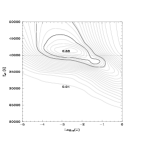
Figure 6: He I 2.06 $\mu$m to Br$\gamma$ line ratio contour plot. The plot was generated from a grid of Cloudy ionization models with varying stellar $T_{\rm eff}$ and ionization parameter, U; see text. The contour interval is 0.04. Basic contours are plotted as grey, while the contours corresponding to $A_{K}=1,3$ mag (0.61 and 0.72, respectively) are plotted as black. The dotted line is an approximate upper limit on $T_{\rm eff}$ based on the larger extent of the Br$\gamma$ emission relative to He I; see text. This plot shows differences from earlier versions of Cloudy; see §3.2.

We computed grids of ionization models parameterized by the $T_{\rm eff}$ of the ionizing source and the ionization parameter, U $\equiv$ $\phi/n(H)c$, where $\phi$ is the number flux of ionizing photons (cm${}^{-2}s^{-1}$), $n(H)$ is the hydrogen density, and $c$ is the speed of light. Thus, for $n,c$ in cm^-3 and cm s^-1, respectively, U is a non–dimensional parameter which sets the ionizing photon number density at the incident cloud face. From the model grids we produced contour plots of the He I 2.06 $\mu$m to Br$\gamma$ line ratio (Figure 6) and the ratio of Br$\gamma$ to far infrared flux (Figure 7). For the latter ratio, we adopt the measurement of Odenwald & Fazio (1984 ) for the far infrared flux (40–250 $\mu$m). Odenwald and Fazio report a size of 1.1^′ for the Sgr D far infrared source. This agrees with the 35^′′ radius we attribute to the H II region; therefore, we compare the fluxes directly. The Br$\gamma$ and He I lines are relatively close in wavelength, so the line ratio does not change a great deal with $A_{K}$. We use the total He I flux in a 15^′′ radius aperture and the corresponding flux from the same size aperture for Br$\gamma$. This gives a ratio of He I to Br$\gamma$ of 0.56 $\pm$ 0.04, which ranges from 0.72 to 0.61 when corrected for reddening (1 $\mathrel{\hbox{\hbox to0.0pt{\hbox{\lower 4.0pt\hbox{$\sim$}}\hss}\hbox{$<$}}}$ $A_{K}$ $\mathrel{\hbox{\hbox to0.0pt{\hbox{\lower 4.0pt\hbox{$\sim$}}\hss}\hbox{$<$}}}$ 3 mag based on the results of § 3.1.1). The ratio of Br$\gamma$ to far infrared flux varies from $4.7\times 10^{-5}$ to $3.1\times 10^{-4}$ for the same range in $A_{K}$. For $A_{K}$ $=$ 1.5 mag, as indicated by the results of §3.1.1, the corrected ratio of He I to Br$\gamma$ is 0.64, and the Br$\gamma$ to far infrared flux ratio is $7.6\times 10^{-5}$.

The $T_{\rm eff}$ of the ionizing radiation field can be estimated from Figures 6 and 7 by overlaying the contours which bracket the observations (for the range of $A_{K}$ taken above). An overlay of the allowed contours from Figures 6 and 7 is shown in Figure 8. We find 36,500 K $\leq$ $T_{\rm eff}$ $\leq$ 40,000 K, in agreement with our rough estimate based on the extent of the He I and Br$\gamma$ emission zones. We have taken 40,000 K as an approximate upper limit to the $T_{\rm eff}$ of the ionizing radiation field based on the fact that the observed Br$\gamma$ emission is more extended than the He I emission (see the discussion above). For the specific case of $A_{K}$ $=$ 1.5 mag, the appropriate contours (0.64 and $7.6\times 10^{-5}$ in Figures 6 and 7, respectively) intersect in Figure 8 at $T_{\rm eff}$$=$ 37,200 K (in the allowed region). The resulting electron temperatures for the models in the overlap region are between $\sim$ $7,000-8,000$ K.

The upper contours in Figure 6 are closed. This indicates the ratio peaks and then begins to fall again at higher $T_{\rm eff}$. This double valued behavior is discussed in detail by Shields (1993) and is due to the complex behavior of the He I line radiative transfer for higher $T_{\rm eff}$ ($\mathrel{\hbox{\hbox to0.0pt{\hbox{\lower 4.0pt\hbox{$\sim$}}\hss}\hbox{$>$}}}$ 40,000 K) of the ionizing source. The physical arguments laid out by Shields remain valid, but the detailed model results (also obtained with Cloudy) for higher $T_{\rm eff}$ have changed slightly since his work due to changes implemented in the Cloudy code. The behavior of the He I to Br$\gamma$ line ratio below $T_{\rm eff}$ $\mathrel{\hbox{\hbox to0.0pt{\hbox{\lower 4.0pt\hbox{$\sim$}}\hss}\hbox{$<$}}}$ 40,000 K is very similar for the present code and the the version used by Shields (1993). The modifications to the current version of Cloudy are discussed by Ferland (1999).

For an ionization bounded H II region and case B conditions, we can estimate the number of ionizing photons required to produce the Br$\gamma$ emission assuming $A_{K}$ $=$ 1.5 mag as indicated by the measurments of stars near the H II region (§3.1.1). Taking the distance to the H II region as 6.0 kpc $\pm^{1.5}_{2.5}$ kpc (§ 3.1.2), gives 48.55 $\leq$ log($Q_{\circ}$ s^-1) $\leq$ 48.99. Liszt (1992) and Mehringer et al. (1998) report 48.31 $\leq$ log($Q_{\circ}$ s^-1) $\leq$ 48.75 and 48.65 $\leq$ log($Q_{\circ}$ s^-1) $\leq$ 49.09, respectively (corrected to the present distance estimate). Therefore, the Br$\gamma$ results are in good agreement with the radio data for the same assumed distance and the estimated $A_{K}$. Alternately, the extinction at 2.17 $\mu$m can be estimated by using the observed radio flux to predict the expected intrinsic Br$\gamma$ flux and then comparing this latter number to the observed Br$\gamma$ flux. We estimate the average extinction at 2.17 $\mu$m by using the predicted Lyman continuum photon luminosity from the radio data (this depends on the integrated radio flux) to estimate the Br$\gamma$ luminosity (e.g., Osterbrock 1989 equation 5$-$23). For case B conditions and $T_{\rm e}$ $=$ 8000 K, the ratio of ionizing photons to Br$\gamma$ luminosity (in cgs) is 7.2$\times$ 10¹³ using the calculations by Hummer & Storey (1987) to determine the Br$\gamma$ effective recombination coefficient. The observed Br$\gamma$ flux is taken from Figure 5 at 35^′′. We find $A_{2.17}$ $=$ 1.01 mag and 1.86 mag using the number of ionizing photons from Liszt (1992) and Mehringer et al. (1998), respectively. This is consistent with the independent measurements of nearby stars found in §3.1.1.

3.3 Location of the H II Region

Lis (1991) and Mehringer et al. (1998) provided strong evidence that Sgr D is not associated with the GC nuclear disk GMCs: the molecular emission and absorption line widths were significantly narrower than for other GMCs in the nuclear disk. Placing Sgr D on either side of the GC is more difficult. Lis (1991) argues that the distance is not less than about 3.5 kpc based on a calculated cloud size and observed angular size. A nearby distance to Sgr D would have important consequences for the star formation rate in the GC (see Lis 1991 for a discussion). Lis also suggested Sgr D could be a feature of the expanding molecular ring, still in the GC region. This fits with the observed CS emission from the cloud associated with the H II region which is at negative velocity (Lis 1991) and perhaps the recombination line velocity which is also negative (Liszt 1992). The latter is less clear since the recombination line is for the extended H II region. Mehringer et al. (1998) argue that the Sgr D H II region could be significantly farther than the GC based on H₂CO absorption by intervening clouds of the extended H II region continuum. This absorption has a large width and positive mean velocity which they associate with a GC cloud. Thus, the Sgr D H II region must be beyond the GC to be seen in absorption. The present narrow–band images appear to rule this out for the compact H II region and dark cloud associated with it.

Our results require a location at least on the near side of the GC. This is essentially because the stellar density in front of the dark cloud is less than half what it is off the cloud (§3.1.2). The stellar distribution peaks so sharply at the GC that the point at which half the stars are observed along a line of sight will be at or before the GC. For the dark cloud on the narrow–band images to occult as many stars as it does, it must be on the near side of the GC. A model which accounts for all the observations is, then, the suggestion of Lis (1991) that the dark cloud associated with the compact H II region is part of the expanding molecular ring. It is in the Galactic center region, but on the near side.

4 SUMMARY

We have presented 2 $\mu$m narrow–band images of the Sgr D H II region including continuum subtracted He I 2.06 $\mu$m and Br$\gamma$ emission lines. The images reveal the compact H II region previously described at far infrared and longer wavelengths. Our images confirm the earlier suggestion by Odenwald (1989) that the H II region is a blister on the edge of a dark cloud. The region in projection against the dark cloud has far fewer stars compared to the other areas of the frame which are crowded with the dense inner Galaxy stellar field. This in itself strongly argues that the cloud must be on the near side of the GC. Our star count models and $A_{K}$ determinations are consistent with a location of the H II region between $\sim$ 3.9 and 7.9 kpc (for a sun–to–GC distance of 8 kpc). A scenario which is consistent with our results and previous molecular line measurements is the suggestion by Lis (1991) that the cloud associated with the compact H II region is located in the expanding molecular ring.

Our analysis of the He I 2.06 $\mu$m emission relative to Br$\gamma$ indicates the ionizing radiation field arises from a source(s) with 36,500 K $\mathrel{\hbox{\hbox to0.0pt{\hbox{\lower 4.0pt\hbox{$\sim$}}\hss}\hbox{$<$}}}$ $T_{\rm eff}$ $\mathrel{\hbox{\hbox to0.0pt{\hbox{\lower 4.0pt\hbox{$\sim$}}\hss}\hbox{$<$}}}$ 40,000 K (for a range of $A_{K}$ of 1 to 3 mag). The upper limit is set by the fact that the Br$\gamma$ emission is more extended than the He I emission. For an $A_{K}$ corresponding to the closest stars in projection to the H II region ($\sim$ 1.5 mag) the derived $T_{\rm eff}$ is 37,200 K. The total number of ionizing photons required to produce the de-reddened Br$\gamma$ luminosity (for an ionization bounded H II region with case B conditions) is in good agreement with previous estimates from radio continuum observations for the same assumed distance to the H II region.

We thank J. Shields and G. Ferland for useful discussions and extensive help with the ionization models. We thank K. Sellgren for useful discussions and a helpful reading of the manuscript. We appreciate the comments and suggestions of an anonymous referee which greatly improved our paper. Support for this work was provided by NASA through grant number HF 01067.01 – 94A from the Space Telescope Science Institute, which is operated by the Association of Universities for Research in Astronomy, Inc., under NASA contract NAS5–26555. A.D. acknowledges financial support received from PRONEX/FINEP. Thanks also to B. Dylan for the new album.

Figure 3: Contour plot of the region surrounding the H II region for the 2.248 $\mu$m continuum (left) and 2.17 $\mu$m (right) images (Figure 1). The contour interval is 1.7$\times$10^-15 erg cm^-2 s^-1 arcsec^-2 and 2.0$\times$10^-15 erg cm^-2 s^-1 arcsec^-2 in the 2.248 $\mu$m and 2.17 $\mu$m plots, respectively. The measured FWHM of point sources is approximately 2.1^′′ and 2.0^′′ for the 2.248 $\mu$m and 2.17 $\mu$m images, respectively. The continuum plot shows three somewhat extended objects (indicated by “cont”) which coincide with the peak Br$\gamma$ emission. The impression is one of embedded sources, one or more of which likely ionize the H II region. We can not rule out the possibility that any or all of these sources is a knot of gas or group of stars. Source “A” is possibly a nearby but foreground star to the H II region; see text. Sources “B” and “C” are potentially young stellar objects associated with the H II region and dark cloud by virtue of their very red color. Alternately, “B” and “C” may be background sources viewed through the large column of material at the edge of the cloud.

Figure 4: $K_{225}$ observed luminosity function. Number of stars detected at three sigma in the 2.248 $\mu$m image as a function of magnitude. The 225 filter is the deepest of the narrow–band images presented here. The star counts appear to rise less steeply at $K_{225}$ $\mathrel{\hbox{\hbox to0.0pt{\hbox{\lower 4.0pt\hbox{$\sim$}}\hss}\hbox{$>$}}}$ 11 mag, which suggests the completeness limit (likely due to crowding) is $\mathrel{\hbox{\hbox to0.0pt{\hbox{\lower 4.0pt\hbox{$\sim$}}\hss}\hbox{$<$}}}$ 11 mag. This is verified by artificial star experiments; see text.

Figure 5: Enclosed flux vs. radius for the Br$\gamma$ (filled triangles) and He I 2.06 $\mu$m (filled squares) emission lines. Both curves have sharp changes in slope which we take to indicate the angular extent of the emission. The smaller extent of the He I emission suggests a relatively cool ionizing continuum. The slight rise in flux beyond 35^′′ in the Br$\gamma$ image is possibly due to the associated extended H II region; see text.

Figure 7: Br$\gamma$ / far infrared dust emission contour plot. The far infrared flux is from Odenwald & Fazio (1984). The plot was generated from a grid of Cloudy ionization models with varying stellar $T_{\rm eff}$ and ionization parameter, U; see text. The contour interval is 2.6$\times$10^-5, and contours above 0.001 are not plotted. Basic contours are plotted as grey, while the contours corresponding to $A_{K}=1,3$ mag (4.7e-5 and 3.1e-4, respectively) are plotted as black.

Figure 8: Overlap region for the allowed contours of Figures 6 and 7. The dotted line represents an approximate upper limit based upon the larger extent to the Br$\gamma$ emission than for the He I emission; see text. For the indicated region outlined by the contours and dotted line, $T_{\rm eff}$ of the ionizing radiation field is approximately 37,000 K to 40,000 K. For a specific case of $A_{K}$ $=$ 1.5 mag (as suggested by measurements of $A_{K}$ for stars projected against the dark cloud), the black dot at 37,200 K represents the intersection of contours for the He I to Br$\gamma$ ratio and the Br$\gamma$ to far infrared flux ratio.

References

- (1)
- (2) Ali, B., Carr, J. S., DePoy, D. L., Frogel, J. A., & Sellgren, K. 1995, AJ, 110, 2415
- (3)
- (4) Anantharamaiah K. R., & Yusef–Zadeh, F. 1989, in IAU Symp. 136, The Center of the Galaxy, ed. M. Morris, (Dordrecht:Kluwer), 159
- (5)
- (6) Bautista, M. A., Pogge, R. W., & DePoy, D. L. 1995, ApJ, 452, 685
- (7)
- (8) Blum, R. D., Carr, J. S., DePoy, D. L., Sellgren, K., & Terndrup D. M. 1994, ApJ, 422, 111
- (9)
- (10) Blum, R. D., DePoy, D. L., & Sellgren, K., 1996, ApJ, 470, 864
- (11)
- (12) Blum, R. D., Sellgren, K., & DePoy, D. L. 1996, AJ, 112, 1988
- (13)
- (14) Blum, R. D., & Damineli, A. 1998, work in progress
- (15)
- (16) Burton, W. B., 1988, in Galactic and Extragalactic Radio Astronomy, ed. G. L. Verschuur & K. I. Kellerman, (New York:Springer–Verlag), 332
- (17)
- (18) Carter, B. S. 1990, MNRAS, 242, 1
- (19)
- (20) Carter, B. S., & Meadows V. S. 1995, MNRAS, 276, 734
- (21)
- (22) Catchpole, R. M., Whitelock, P. A., & Glass, I. S. 1990, MNRAS, 247, 479
- (23)
- (24) Downes, D., Goss, W. M., Schwartz, U. J., & Wouterloot, J. G. A. 1978, A&A, 35, 1
- (25)
- (26) Elias, J. H., Frogel, J. A., Matthews, K., & Neugebauer, G. 1982, AJ, 87, 1029
- (27)
- (28) Ferland, G. J. 1996, Hazy, A Brief Introduction to Cloudy, University of Kentucky, Department of Physics and Astronomy Internal Report
- (29)
- (30) Ferland, G. J. 1999, ApJ in Press
- (31)
- (32) Hanson, M. M., Conti, P. S., & Rieke, M. J. 1996, ApJS, 107, 281
- (33)
- (34) Hummer, D. G. & Storey P. J. 1987, MNRAS, 224, 801
- (35)
- (36) Johnson, H. 1966, ARA&A, 4, 193
- (37)
- (38) Kázes I., & Aubry, D., 1973, A&A, 22, 413
- (39)
- (40) Kent, S. M., 1992, ApJ, 387, 181
- (41)
- (42) Kurucz, R. L. 1991, in Proceedings of the Workshop on Precision Photometry: Astrophysics of the Galaxy, eds. A. C. Davis Phillip, A. R. Upgren, & K. A. James, (Davis: Schenectady), 27
- (43)
- (44) Lis, D. C. 1991, ApJ, L53
- (45)
- (46) Liszt, H. S. 1992, ApJS, 82, 495
- (47)
- (48) Mathis, J.S. 1990, ARA&A, 28, 37
- (49)
- (50) Mehringer, D. M., Goss, W. M., Lis, D. C., Palmer, P., Menten, K. M. 1998, ApJ, 493, 274
- (51)
- (52) Odenwald, S. F. 1989, in IAU Symp. 136, The Center of the Galaxy, ed. M. Morris, (Dordrecht:Kluwer), 205
- (53)
- (54) Odenwald, S. F., & Fazio G. G. 1984, ApJ, 283, 601
- (55)
- (56) Osterbrock, D. E. 1989, Astrophysics of Gaseous Nebulae and Active Galactic Nuclei, (Mill Valley, California:University Science Books), 30
- (57)
- (58) Schecter, P. L., Mateo, M. L., & Saha, A. 1993, PASP, 105, 1342
- (59)
- (60) Shields, J. C. 1993, ApJ, 419, 181
- (61)
- (62) Terndrup, D. M., Frogel, J. A., & Whitford, A. E. 1991, ApJ, 378, 742
- (63)
- (64) Whiteoak, J. B. & Gardner F. F. 1974, A&A, 37, 389
- (65)