The Supergalactic Plane revisited with the Optical Redshift Survey

Abstract

We re-examine the existence and extent of the planar structure in the local galaxy density field, the so-called Supergalactic Plane (SGP). This structure is studied here in three dimensions using both the new Optical Redshift Survey (ORS) and the IRAS 1.2 Jy redshift survey. The density contrast in a slab of thickness of $20{\,h^{-1}\,{\rm Mpc}}$ and diameter of $80{\,h^{-1}\,{\rm Mpc}}$ aligned with the standard de Vaucouleurs’ Supergalactic coordinates, is $\delta_{sgp}\sim 0.5$ for both ORS and IRAS. The structure of the SGP is not well described by a homogeneous ellipsoid, although it does appear to be a flattened structure, which we quantify by calculating the moment of inertia tensor of the density field. The directions of the principal axes vary with radius, but the minor axis remains within $\theta_{z}\sim 30^{\circ}$ of the standard SGP $Z$-axis, out to a radius of $80{\,h^{-1}\,{\rm Mpc}}$, for both ORS and IRAS. However, the structure changes shape with radius, varying between a flattened pancake and a dumbbell, the latter at a radius of $\sim 50{\,h^{-1}\,{\rm Mpc}}$, where the Great Attractor and Perseus-Pisces superclusters dominate the distribution. This calls to question the connectivity of the ‘plane’ beyond $\sim 40{\,h^{-1}\,{\rm Mpc}}$. The configuration found here can be viewed as part of a web of filaments and sheets, rather than as an isolated pancake-like structure. An optimal minimum variance reconstruction of the density field using Wiener filtering which corrects for both redshift distortion and shot noise, yields a similar misalignment angle and behaviour of axes. The background-independent statistic of axes proposed here can be best used for testing cosmological models by comparison with $N$-body simulations.

1 Introduction

The major planar structure in the local universe, the Supergalactic Plane (SGP), was recognized by de Vaucouleurs (1953, 1956, 1958, 1975a,b) using the Shapley-Ames catalogue, following an earlier analysis of radial velocities of nearby galaxies which suggested a differential rotation of the ‘metagalaxy’ by Rubin (1951). This remarkable feature in the distribution of nebulae was in fact already noticed by William Herschel more than 200 years earlier (for historical reviews see Flin 1986, Rubin 1989).

When referring to the SGP in this paper we mean the planar structure in the galaxy distribution. This should be distinguished from the formal definition of Supergalactic coordinates.  de Vaucouleurs et al.  (1976, 1991) defined a spherical coordinate system $L,B$ in which the equator roughly lies along the SGP (as identified at the time), with the North Pole ($B=90^{\circ}$) in the direction of Galactic coordinates ($l=47.37^{\circ};b=+6.32^{\circ}$). The position $L=0^{\circ},B=0^{\circ}$ is at ($l=137.37^{\circ},b=0^{\circ}$), which is one of the two regions where the SGP is crossed by the Galactic Plane. The Virgo cluster is at ($L=104^{\circ};B=-2^{\circ}$). Traditionally, the Virgo cluster was regarded as the centre of an overdense region called the ‘Local Supercluster’ (e.g. Davis & Huchra 1982, Hoffman & Salpeter 1982, Tully & Shaya 1984, Lilje, Yahil & Jones 1986). However, some of the much larger superclusters that are seen in recent redshift surveys, such as the Great Attractor and Perseus-Pisces, are near the SGP, and are possibly connected with the Local Supercluster, in the sense of being simply connected by an isodensity contour above the mean density (cf., Strauss et al.  1992; Strauss & Willick 1995; Santiago et al.  1995).

Although the SGP is clearly visible in whole-sky galaxy catalogues (e.g. Lynden-Bell & Lahav 1988; Lynden-Bell et al.  1988; Raychaudhury 1989; see also the references above), the extent of planar structure in the galaxy distribution in 3 dimensions has seen little quantitative examination in recent years. Tully (1986, 1987) claimed that the flattened distribution of clusters extends across a diameter of $\sim 0.1c$ with axial ratios of 4:2:1. Shaver & Pierre (1989) found that radio galaxies are more strongly concentrated to the SGP than are optical galaxies, and that the SGP as represented by radio galaxies extends out to redshift $z\sim 0.02$. Stanev et al.  (1995) claimed that energetic cosmic rays arrive preferentially from the direction of the SGP, where potential sources (e.g. radio galaxies) are concentrated, but this result was criticized by Waxman, Fisher & Piran (1997). Di Nella & Paturel (1995) revisited the SGP using a compilation of nearly 5700 galaxies larger than 1.6 arcmin, and found indeed that galaxies were concentrated close to the Supergalactic Plane. Loan (1997) and Baleisis et al.  (1998) searched for the SGP in projection in the 87GB (north) and PMN (south) radio surveys, and found signatures at the 1 and 3 $\sigma$ levels, respectively.

The existence of a pancake-like structure has important theoretical implications. Gravity amplifies deviations from sphericity, i.e. an initial oblate homogeneous ellipsoid evolves into a disk, and an initial prolate structure ends up as a spindle (Lin, Mestel & Shu 1965). White & Silk (1979) modeled the Local Supercluster as a homogeneous ellipsoid in expanding universe, and considered implications for cosmological models and initial conditions. Although such a simple model is insightful, the structure of the SGP is far more complicated than a homogeneous ellipsoid, as we show below. In a more realistic cosmological scenario, where the primordial density field is Gaussian, non-spherical shapes are more abundant than spherical ones (Doroshkevich 1970, Bardeen et al.  1986), and hence are expected to appear at the present epoch as even more non-spherical. In the context of the ‘top-down’ Hot Dark Matter scenario, Zel’dovich (1970) showed that pancake-like structures are the natural outcome of gravitational instability in the quasi-linear regime. Further studies have indicated that a web of filaments could also form in hierarchical Cold Dark Matter (bottom-up) scenarios (e.g. Bond, Kofman & Pogosyan 1996), but the shapes look quite different in different scenarios, as a result of both initial conditions and the cosmic time which allows the perturbations to grow. Hence, quantitative measures of the SGP and other observed filamentary structures and superclusters (Bahcall 1988) could be very important in distinguishing between models, e.g. by applying the shape statistic to both data and to $N$-body simulations.

Here we study the properties of the SGP using the Optical Redshift Survey (ORS, Santiago et al.  1995) which provides the most detailed and uniform optically-selected sample of the local galaxy density field to date. For comparison, we also use the full-sky redshift survey of galaxies selected from the database of the Infrared Astronomical Satellite (IRAS), complete to 1.2 Jy at 60$\mu$m (Fisher et al.  1995a). In this paper we consider the approach of ‘moment of inertia’ (MoI) to quantify a planar structure (cf. Babul & Starkman 1992; Luo & Vishniac 1995; Dave et al.  1997; Sathyaprakash et al.  1998).

The outline of the paper is as follows. Section 2 describes the ORS and IRAS  samples, while in Section 3 we discuss the visual impression and preliminary analysis of the SGP. Section 4 describes the formalism of the MoI we also develop related statistics which are independent of the background determination. Section 5 gives the results of MoI when applied to the samples, and Section 6 presents Wiener reconstruction of the MoI for IRAS. Section 7 gives interpretation of the results using mock realizations, and conclusions and future work are discussed in Section 8.

2 The ORS and IRAS  samples

The Optical Redshift Survey (ORS, Santiago et al.  1995) covers the sky at Galactic latitude $|b|>20^{\circ}$. The survey was drawn from the UGC (Nilson 1973), ESO (Lauberts 1982), and ESGC (Corwin & Skiff 1995) galaxy catalogues, and it contains two subsets: one complete to a blue photographic magnitude of 14.5, and the other complete to a blue major diameter of 1.9 arcmin. The entire sample consists of 8457 galaxies, with redshifts available for 98% of them; $\approx 1300$ new redshifts were measured to complete the survey. The high number density of galaxies in ORS makes it ideal for cosmographical studies of the local universe.

As ORS only covers $|b|>20^{\circ}$, we filled in the Zone of Avoidance (ZOA) at $|b|<20^{\circ}$ with galaxies from the IRAS  1.2 Jy survey (Fisher et al.  1995a). The Zone of Avoidance in IRAS, $|b|<5^{\circ}$, was filled by interpolation based on the observed galaxy distribution below and above the ZOA (Yahil et al.  1991). While in principle it is possible to interpolate for the ORS ZOA, e.g. by hand or using a Wiener reconstruction (Lahav et al.  1994), we prefer to include real structure as probed by IRAS  even at the price of mixing two different data sets. Hereafter when we refer to the ORS sample we mean that supplemented by the IRAS 1.2 Jy galaxies at $|b|<20^{\circ}$.

Due to Galactic extinction and the diversity of catalogues used, the selection function of ORS depends on both distance and direction (Santiago et al.  1996). In order to account for these selection effects, a weight is usually associated with each galaxy. For a uniform survey like IRAS (see below) the selection function $\phi$ depends only on the distance to a galaxy, $|{\bf x}|$, and hence the weight is simply

$$w_{gal}={1\over{\langle n\rangle\phi(|{\bf x}|)}},$$

where the mean number density of galaxies is estimated by

$$\langle n\rangle={1\over V}\sum_{gal}1/\phi(|{\bf x}|)\;$$

(see Davis & Huchra 1982 for an alternative minimum variance estimator of the mean density).

For ORS, we follow Santiago et al.  (1996) and Hermit et al.  (1996) and weight each galaxy by:

$$w_{gal}={1\over{\langle n\rangle_{\mu}\phi({\bf x})}}\;{\langle n\rangle_{\mu,iras}\over\langle n\rangle_{tot,iras}}\;,$$

where $\mu$ labels the catalogue from which the galaxy in question is drawn; each of the four catalogues making up the ORS has its own mean density $\langle n\rangle_{\mu}$. Here $\langle n\rangle_{\mu,iras}$ is the mean number density of IRAS galaxies in the volume corresponding to the $\mu$-th catalogue in ORS. This brings each of the subsamples, with their separate selection criteria, to a uniform weighting (Santiago et al.  1996). With the weighting of equation (1) or (3), we can thus calculate the galaxy density fluctuation field $\delta({\bf x})\equiv(\rho({\bf x})-\langle\rho\rangle)/\langle\rho\rangle$ throughout the volume surveyed.

For comparison we also apply our analysis to the complete IRAS  1.2 Jy sample (Fisher et al.  1995a; Strauss et al.  1992), which includes 5313 galaxies over 87.6 % of the sky. The ZOA in IRAS  was interpolated according to the Yahil et al.  (1991) procedure mentioned above. Hereafter we refer to this sample as the IRAS  sample. We note that the ORS and IRAS samples are not really independent; roughly 60% of the IRAS 1.2 Jy galaxies out to $80{\,h^{-1}\,{\rm Mpc}}$ are also catalogued in the ORS magnitude limited sample.

We work purely in Local Group redshift space, except in section 6 on Wiener reconstruction.

3 A BRIEF TOUR OF THE SGP

3.1 Visual impression

Historically, the SGP was identified in projected 2-D maps. We used the IRAS sample (which is homogeneous over the sky) to revisit the 2-D appearance of the SGP by fitting the data to a great circle. For a projected distribution of sources the great circle along which the density of galaxies is enhanced can be found by calculating the covariance matrix: $I_{ij}=\sum_{gal}{\hat{x}_{i}}{\hat{x}_{j}}$ where the Cartesian axes ${\hat{x}_{i}}$ ($i=1,2,3$) are defined for a unit sphere. The matrix $I_{ij}$ can be diagonalised (cf. Section 4.2) and the smallest eigen-vector indicates the direction of the normal to the great circle. We considered the projected IRAS galaxy distribution out to $40{\,h^{-1}\,{\rm Mpc}}$ and $80{\,h^{-1}\,{\rm Mpc}}$, and found that the great circle is aligned with the standard de Vaucouleurs’ SGP to within $19^{\circ}$ and $7^{\circ}$ respectively. Can we see the translation of the great circle to a plane in 3-dimensions? Figure 1 shows the raw distributions, uncorrected for selection effects of ORS and IRAS galaxies in a sphere of radius of $40{\,h^{-1}\,{\rm Mpc}}$ projected on the standard ($SGX$-$SGZ$), ($SGX$-$SGY$) and ($SGY$-$SGZ$) planes. The SGP is particularly visible edge-on in the ($SGX$-$SGZ$) and ($SGY$-$SGZ$) projections. We note that the structures seen in ORS and IRAS are quite similar, but the ORS map is much denser, and clusters are more prominent.

Figure 1: The distributions of ORS and IRAS  galaxies in a sphere of radius of $40{\,h^{-1}\,{\rm Mpc}}$, projected on the standard ($SGX$-$SGZ$), ($SGX$-$SGY$) and ($SGY$-$SGZ$) planes. The SGP is visible edge-on as the linear feature at $SGZ=0$ in the ($SGX$-$SGZ$) and ($SGY$-$SGZ$) projections.

Maps of the smoothed density field, after applying the appropriate weights, are shown elsewhere for the IRAS survey (Saunders et al.  1991; Strauss et al.  1992; Fisher et al.  1995b; Strauss & Willick 1995; Webster, Lahav & Fisher 1997) and for ORS (Santiago et al.  1995, 1996; Baker et al.  1998). In Figures 2 and 3 we show histograms of the galaxy density field $\delta$, corrected for selection effects, as a function of $SGZ$, averaged over $SGX$ and $SGY$, within spheres of ever-larger radii, as indicated in each panel. The SGP is seen as an enhancement at $SGZ=0$ in these plots to roughly $R_{max}=60{\,h^{-1}\,{\rm Mpc}}$, but is not apparent on larger scales.

Figure 2: Histograms of the ORS density field (corrected for selection effects) as a function of $SGZ$, averaged over $SGX$ and $SGY$, within spheres of radius as indicated in each panel. The error bars are Poissonian.

Figure 3: Histograms of the IRAS density field (corrected for selection effects) as a function of $SGZ$, averaged over $SGX$ and $SGY$, within spheres of radius as indicated in each panel. The error bars are Poissonian.

3.2 The level of overdensity

Our visual impression is that there is indeed a flattened structure in the galaxy distribution, aligned along $SGZ=0$, extending to appreciable redshifts. To quantify this we calculate the overdensity $\delta_{sgp}\equiv n_{sgp}/\langle n\rangle-1$ as a function of $R_{max}$, where $n_{sgp}$ is evaluated within a circular cylinder centered on the Local Group with radius $R_{max}$ and height along SGZ of $20{\,h^{-1}\,{\rm Mpc}}$, and the mean density $\langle n\rangle$ is calculated within a sphere of radius $R_{max}$ (including the slab). This overdensity reaches a maximum at $R_{max}=40{\,h^{-1}\,{\rm Mpc}}$ (for which the volume of the slab is $\sim(46{\,h^{-1}\,{\rm Mpc}})^{3}$), $\delta_{sgp}(40)=0.48\pm 0.06$ and $0.46\pm 0.09$ for ORS and IRAS, respectively. At $R_{max}=60{\,h^{-1}\,{\rm Mpc}}$, $\delta_{sgp}(60)=0.36\pm 0.06$ and $0.26\pm 0.08$ for ORS and IRAS, respectively. For reference, the rms fluctuations in cubes of volume $(40{\,h^{-1}\,{\rm Mpc}})^{3}$ are $\delta_{rms}\sim 0.37$ and $\sim 0.30$ for optical (Stromlo/APM) and IRAS (1.2 Jy) surveys, respectively (Efstathiou 1993). Hence the fluctuation in galaxy counts in a slab aligned with the standard de Vaucouleurs’ SGP is no more than $\sim 1.5\,\sigma$ perturbation on scale of $\sim 40{\,h^{-1}\,{\rm Mpc}}$. This implies that the SGP is only a modest perturbation on these large scales. The overdensity as a function of the $Z$ component of the standard SGP is depicted in Figures 2 and 3.

3.3 The centre of the overdensity

In order to quantify the local overdensity, we need to calculate the centre of ‘mass’ of the density field, within a sphere of radius $R_{max}$ centred on us, for both the ORS and IRAS samples (cf., Juszkiewicz et al.  1990). The centre of mass is given by summing over the galaxies (assuming they all have equal mass):

$${\bar{x}_{i}}={1\over V}\sum_{gal}w_{gal}\;x_{i}\;,$$

where $i=1,2,3$, $V$ is the total volume of the sphere of radius $R_{max}$ and $w_{gal}$ is the weight per galaxy described in §2. The shot noise error in each axis is

$$\sigma_{\bar{x}}^{2}={1\over V^{2}}\sum_{gal}w_{gal}^{2}\;x_{i}^{2}={1\over 3V^{2}}\sum_{gal}w_{gal}^{2}\;r^{2},$$

where the last equality is valid for an isotropic distribution. Figure 4 shows the coordinates of the centre of the galaxy distribution as a function of $R_{max}$. The centre moves away from the origin (the Local Group) by no more than $8{\,h^{-1}\,{\rm Mpc}}$ for ORS and $6{\,h^{-1}\,{\rm Mpc}}$ for IRAS. This is partially due to the ‘tug of war’ between the Great Attractor and Perseus-Pisces, which largely balance each other out. Indeed, the centre moves back towards the origin for $R_{max}>40{\,h^{-1}\,{\rm Mpc}}$.

Figure 4: The variation of the mean position of the centre of mass of the galaxy distribution within a sphere of radius $R_{max}$ centred on us, for both the ORS and IRAS samples. The curves show the Supergalactic $x,y,z$ of the centre of mass, and its radial distance from the origin.

4 Principal Components of the Inertia Tensor

Both visual impression of and a formal $\chi^{2}$ fit suggest that the SGP cannot be fitted by a homogeneous ellipsoid model. We therefore seek a more objective measure of deviation from sphericity, via the Moment of Inertia tensor (MoI).

4.1 Estimation of the Moment of Inertia

We wish to detect a high density planar structure (e.g. a slab or an ellipsoid) embedded in a uniform sphere of radius $R_{max}$. One approach (cf. Babul & Starkman 1992, Luo & Vishniac 1995, Dave et al.  1997) is to construct the MoI for the fluctuation in the density field:

$${\tilde{C}_{ij}}=\;C_{ij}-{\bar{C_{ij}}}=\;{1\over{\langle n\rangle V}}\int[n({\bf x})-n_{bg}](x_{i}-{\bar{x}_{i}})(x_{j}-{\bar{x}_{j}})\;dV,$$

where $n({\bf x})$ is the galaxy number density at position ${\bf x}$, $\langle n\rangle$ is the mean number density and $x_{i},x_{j}$ ($i,j=1,2,3$) are Cartesian components of ${\bf x}$. Note that we allow the centre $\bar{\bf x}$ to move (see Figure 4), although below, we will end up keeping it fixed. The integration is over the volume of the sphere. We define the fluctuations in the density field relative to the background density $n_{bg}$ in the absence of the slab (which differs from the mean density $\langle n\rangle$ including the slab).

For a uniform distribution with density $\langle n\rangle$ the covariance matrix is analytic and isotropic:

$${\bar{C}_{ij}}={f_{bg}\over V}\int x_{i}x_{j}dV={1\over 3}\delta_{ij}^{K}{f_{bg}\over V}\int_{0}^{R_{max}}r^{2}(4\pi r^{2}dr)=$$

$$=\delta_{ij}^{K}\;f_{bg}\;{R_{max}^{2}\over 5},$$

where

$$f_{bg}\equiv{n_{bg}\over{\langle n\rangle}},$$

$\bar{\bf x}$ is of course zero, and $\delta_{ij}^{K}$ is the Kronecker delta function.

For a discrete density field, such as provided by ORS or IRAS , we can calculate the covariance elements by summing over the galaxies:

$${\tilde{C}_{ij}}=C_{ij}-{\bar{C}_{ij}}={1\over V}\sum_{gal}w_{gal}x_{i}x_{j}-\delta_{ij}^{K}f_{bg}{R_{max}^{2}\over 5}\;,$$

where we have set $\bar{\bf x}=0$, given the fact that the centre of mass stays so close to the origin (Figure 4). An analytic estimator for Poisson shot-noise per diagonal component of the covariance matrix (assuming no errors in $f_{bg}$) is:

$$\sigma_{c}^{2}={1\over{(3V)}^{2}}\sum_{gal}w_{gal}^{2}\;r^{4}\;.$$

Eq. (9) requires knowledge of $f_{bg}$ in order to correct for the background density. However, as the boundaries of the SGP are hard to define a priori and the background will not be uniform, it is difficult to estimate a meaningful $f_{bg}$. In §4.3 we suggest a statistic which is independent of this parameter.

4.2 Principal axes

The next step in our analysis is to diagonalize the MoI and find the eigenvalues $\lambda_{\alpha}$ and associated eigenvectors ${\bf u}_{\alpha}$ ($\alpha=1,2,3$):

$${\tilde{C}}{\bf u}_{\alpha}=\lambda_{\alpha}{\bf u}_{\alpha}\;.$$

The standard deviation (‘1-$\sigma$’) along each of the three axes is given by $\sqrt{\lambda_{\alpha}}$, which we label hereafter as $a,b,c$. Note that since the background contribution (the last term in eq. 9) is isotropic, it only affects the eigenvalues, but not the directions of the eigenvectors. This procedure is essentially the Principal Component Analysis (PCA) - a well known statistical tool for reducing the dimensionality of parameter space (e.g. Murtagh & Heck 1987 and references therein). By identifying the linear combination of input parameters with maximum variance, PCA determines the Principal Components that can be most effectively used to characterize the input data. In our case, in searching for a plane, we wish to see if the PCA finds one axis to be much shorter than the other two axes.

4.3 Background-independent statistic of axes

Our aim is to quantify deviations from spherical structure. The difficulty in doing so is due to two problems: (i) the background density as modeled above with $f_{bg}$ is ill-determined, and (ii) the shot noise due to the finite number of galaxies can be quite large.

We will discuss the shot noise problem in §6 below. To overcome the problem of the unknown background, we can construct the following quantities which are independent of $f_{bg}$:

$$p^{2}=|a^{2}-b^{2}|\;,$$

$$q^{2}=|a^{2}-c^{2}|\;.$$

and

$$s^{2}=|b^{2}-c^{2}|\;.$$

For a perfect sphere, $p=q=s=0$. For a homogeneous oblate ellipsoid with semi-major axes $A=B>C$, one expects $p=0$ for all $R_{max}$, but for $q$ and $s$ to increase out to $R_{max}\approx A$ and then to decline. Note that the $(p,q,s)$ here are in the diagonalized PCA frame, where the axes are ordered by size ($a\geq b\geq c$). Alternatively, we can calculate $(p,q,s)$ along fixed $(x,y,z)$ axes (e.g. in de Vaucouleurs’ system) by replacing $a^{2},b^{2},c^{2}$ in eqs. (12-14) by the non-ordered variances in that fixed coordinate system (i.e. the diagonal elements in the MoI matrix in that $(x,y,z)$ coordinate system).

In the limit that the errors are isotropic the Poisson error bars are:

$$\Delta p=\sigma_{c}^{2}/p\;,$$

and similarly for $q$ and $s$. We will determine the characteristic shape of the galaxy density field, from the observed $p,q$ and $s$ and their error bars as a function of $R_{max}$. We note that other transformations of $(a,b,c)$ are possible, such as the $(S1,S2,S3)$ statistic proposed by Babul & Starkman (1992).

4.4 Mock realizations

To get an insight into our $(p,q,s)$ statistic we applied it to mock realizations of ellipsoids placed in a uniform background. The IRAS selection function was applied to the mock samples, and the results were averaged over 100 realizations. Figure 5 shows the quantities $p,q$, and $s$ derived at fixed axes for mock ellipsoids (oblate, prolate and triaxial) with dimensions indicated in the panels and overdensity of $\delta=0.4$. When the axes were allowed to be chosen by PCA, the axes agreed with the correct orientation of the ellipsoids to within $7^{\circ}$ (rms over 100 realizations). For a single realization the curves are much more noisy. Moreover, if PCA defines the axes, it attempts to maximize the differences between the axes, and the results for $p,q$, and $s$ are biased by noise. For example, in the case of a perfectly oblate structure in the presence of noise, the quantity $s$ increases with radius $R_{max}$, where it is identically zero in the noise-free case. Fortunately, we will see in the following section that the behaviour of $(p,q,s)$ for the real data is quite robust. We will continue these experiments with the mock realizations in §7, where we consider more complex geometries.

Figure 5: The quantities $p$ (crosses), $q$ (open squares) and $s$ (filled circles) given by eqs. (12-14) vs. $R_{max}$ for mock ellipsoids (oblate, prolate and triaxial) with dimensions (in ${\,h^{-1}\,{\rm Mpc}}$) indicated in the panels, all ellipsoids with density contrast of $\delta=0.4$. The mock samples have an IRAS selection function, and the results are averaged over 100 realizations at fixed axes.

5 Application of MoI to ORS and IRAS

We now apply the MoI approach to the ORS and IRAS samples. We begin by considering $p,q,$ and $s$ along fixed axes. We will find below that the PCA direction at small $R_{max}$ is indeed very close to that of de Vaucouleurs’ system, so we simply choose the standard de Vaucouleurs’ SGP axes. Figure 6 shows $p,q$ and $s$ (derived here from the variances along the standard SGP axes without ordering them, as explained in section 4.3) as a function of $R_{max}$. The most notable feature is the dip in $s$ at about $R_{max}=50{\,h^{-1}\,{\rm Mpc}}$ in both samples. This is due to the dumbbell-like configuration of Perseus-Pisces and the Great Attractor on opposite sides of the sky, as we’ll see in §7. But at $R_{max}=80{\,h^{-1}\,{\rm Mpc}}$, the structure is pancake-like: $p$ tends to small values (in particular in ORS), more in line with the visual impression of a pancake-like structure in Figure 1. However, the dramatic changes with $R_{max}$ (in particular at $50{\,h^{-1}\,{\rm Mpc}}$) call to question the notion of a single coherent feature within the boundaries of our samples (see §7). Based on Figure 6, one may argue that the ‘plane’ terminates at $\sim 40{\,h^{-1}\,{\rm Mpc}}$.

We now turn to the PCA approach of diagonalizing the MoI derived at each radius $R_{max}$. In this case the axes change direction, and might even ‘swap’. ’Swapping’ means that an axis which is the largest at a given $R_{max}$ may become say the second or third largest in a different $R_{max}$. Hence we may see a discontinuity in the variation of the ‘largest’ axis with $R_{max}$.

The variation at large $R_{max}$ is more difficult to interpret, but we see that $q>p>s$, implying a triaxial shape, and $p$ and $q$ increase with $R_{max}$. In contrast, the toy models (Figure 5) show that two of $[p,q,s]$ drop with $R_{max}$ beyond the radius which encloses the ellipsoid ($80{\,h^{-1}\,{\rm Mpc}}$ in the toy models). But in making this comparison with Figure 5 we should keep in mind that at large $R_{max}$ the increase of the observed quantities $p,q$ or $s$ might be due to shot-noise. It is also interesting to note the similarity between ORS and IRAS, indicating that on the very large scales the density fields in the two samples are quite similar.

Table 1 lists $a,b,c$, their Poisson errors, and the direction of the PCA $Z$ component for ORS (for direct summation) and IRAS (for both direct summation and Wiener reconstruction described in the next Section). Table 1 also lists the values in differential shells, showing trends similar to those seen in the cumulative plots.

Fig 9 shows the variation of direction of the PCA $Z$ component with $R_{max}$. We see that although the angle $\theta_{z}\equiv 90^{\circ}-B_{z}$ between the PCA minor axis and de Vaucouleurs’ pole is usually less than $30^{\circ}$, there is a significant variation on the sky (relative to the errors of $\sim 10^{\circ}$ due to shot noise). Particularly noticeable is the big jump at $R_{max}=50{\,h^{-1}\,{\rm Mpc}}$, in accord with the behaviour in Figures 6,7 and 8. This is again due to the dumbbell configuration of the Great Attractor and the Perseus-Pisces superclusters, as we shall see in §7. Table 1 also gives $B_{z}$, the complement of the misalignment angle $\theta_{z}$, for 3 shells, each 20 $h^{-1}\,$ Mpc wide. We see that indeed typically $\theta_{z}\sim 30^{\circ}$, even at the (60-80) $h^{-1}\,$ Mpc shell, which is beyond the Great Attractor and Perseus-Pisces. The probability that two random vectors are separated by an angle less than $\theta_{z}\sim 30^{\circ}$ by chance is $P(<\theta_{z})=[1-\cos(\theta_{z})]$, i.e. $\sim 13\%$.

Figure 6: The quantities $(p,q,s)$ derived from the variances along the de Vaucouleurs’ axes vs. $R_{max}$ (cumulative) for the ORS and IRAS samples. The error bars are Poisson.

Figure 7: The quantities $(p,q,s)$ derived from PCA dimensions $(a,b,c)$ (eqs. 12-14) vs. $R_{max}$ (cumulative) for the ORS and IRAS samples. The error bars are Poisson.

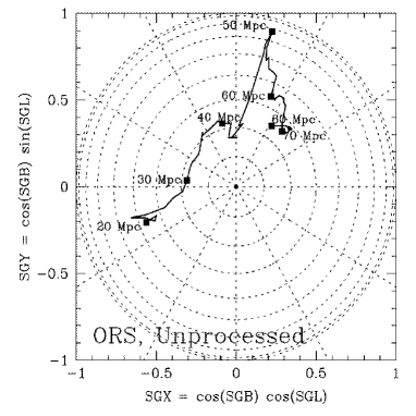
Figure 8: ORS : The direction of the $Z$ axis from the PCA analysis (using direct summation over the galaxies) relative to the de Vaucouleurs’ pole. Values of $R_{max}$ are indicated.

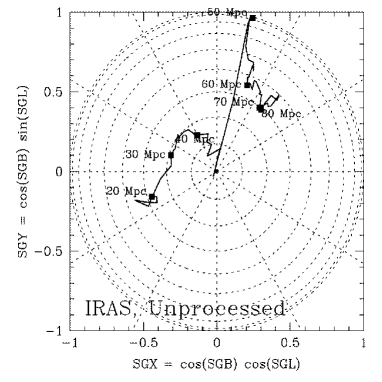
Figure 9: IRAS : The direction of the $Z$ axis from the PCA analysis (using direct summation over the galaxies) relative to the de Vaucouleurs’ pole. Values of $R_{max}$ are indicated.

Figure 10: The quantities $p,q,s$ vs. $R_{max}$ (cumulative) in PCA axes using spherical harmonic reconstruction of IRAS and analytic MoI. Top: corrected for redshift distortion and noise by Wiener filtering, with parameters $\beta=0.7,\Gamma=0.2,\sigma_{8}=0.7$ (reconstruction out to 200 $h^{-1}\,$ Mpc). Bottom : using raw harmonics.

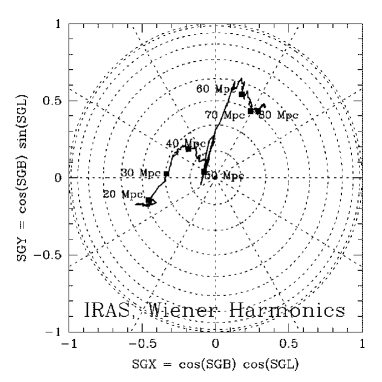
Figure 11: Wiener filtering of IRAS : The direction of the $Z$ axis (as found by PCA) relative to the de Vaucouleurs’ pole. Values of $R_{max}$ are indicated.

Table 1. SGP parameters from PCA analysis

  $R_{min}$ $R_{max}$ $a$ $b$ $c$ $\Delta(a^{2})$ $L_{z}$ $B_{z}$ ORS
0 20 9.9 8.1 7.1 2.4 160 53 0 30 14.8 12.4 11.0 5.1 173 72 0 40 19.9 16.2 14.3 7.7 104 68 0 50 25.8 20.7 20.0 12.7 76 23 0 60 31.8 26.5 22.7 17.8 67 56 0 70 35.6 31.1 27.0 24.1 48 65 0 80 39.8 35.2 31.0 33.0 58 65 20 40 21.7 17.7 15.4 9.5 101 66 40 60 35.1 29.2 24.8 23.7 65 55 60 80 45.8 40.3 36.2 57.4 52 68 IRAS
0 20 10.3 8.1 7.2 3.4 160 62 0 30 14.9 13.0 11.1 6.6 162 71 0 40 19.6 16.8 14.7 10.6 120 75 0 50 25.5 21.3 20.8 16.4 76 -6 0 60 31.2 26.5 23.6 21.9 69 55 0 70 35.1 30.7 27.9 29.3 54 60 0 80 39.6 35.3 32.8 39.0 52 61 20 40 21.3 18.0 15.8 12.8 113 72 40 60 34.2 29.0 25.8 28.8 67 53 60 80 44.9 40.5 38.3 65.9 44 60 IRAS Wiener
0 20 10.1 8.5 7.8 - 197 61 0 30 14.6 13.4 11.9 - 176 70 0 40 19.5 17.6 15.9 - 135 75 0 50 24.5 21.4 21.2 - 154 85 0 60 29.7 26.2 24.6 - 72 55 0 70 34.0 30.8 29.0 - 61 60 0 80 38.3 35.3 33.5 - 56 59  

Comments on Table 1: $R_{min}$, $R_{max}$, $a,b$ and $c$ are in $h^{-1}$ Mpc. The values of $a,b$ and $c$ are for $f_{bg}=0$. The Poisson error per axis $\Delta(a^{2})$ is derived using eqs. (15-17). No errors are given in the Wiener case, as this is a smoothed field (although one can calculate the scatter around the mean).

$L_{z}$ and $B_{z}$ (both in degrees) give the direction in standard de Vaucouleurs’ coordinates of the $Z$ component as found by PCA. The angle between this direction and de Vaucouleurs’ SGP pole is simply $\theta_{z}=90^{\circ}-B_{z}$.