CONSTRAINING $q_{0}$ WITH CLUSTER GAS MASS FRACTIONS: A FEASIBILITY STUDY

Abstract

As the largest gravitationally bound objects in the universe, clusters of galaxies may contain a fair sample of the baryonic mass fraction of the universe. Since the gas mass fraction from the hot ICM is believed to be constant in time, the value of the cosmological deceleration parameter $q_{0}$ can be determined, in principle, by comparing the calculated gas mass fraction in nearby and distant clusters (Pen 1997). To test the potential of this method, we compare the gas fractions derived for a sample of luminous ($L_{X}>10^{45}$erg s^-1), nearby clusters with those calculated for eight luminous, distant ($0.3<z<0.6$) clusters using $ASCA$ and $ROSAT$ observations. For consistency, we evaluate the gas mass fraction at a fixed physical radius of 1 $h_{50}^{-1}$ Mpc (assuming $q_{0}$=0.0). We find a best fit value of $q_{0}=0.07$ with -0.47 $<q_{0}<$ 0.67 at 95% confidence. This analysis includes both measurement errors and an intrinsic 25% scatter in the gas fractions due to the effects of cooling flows and mergers. We also determine the gas fraction using the method of Evrard, Metzler, & Navarro (1997) to find the total mass within $r_{500}$, the radius where the mean overdensity of matter is 500 times the critical density. In simulations, this method reduces the scatter in the determination of gravitational mass without biasing the mean. We find that it also reduces the scatter in actual observations for nearby clusters, but not as much as simulations suggest. Using this method, the best fit value is $q_{0}=0.04$ with -0.50 $<q_{0}<$ 0.64. The excellent agreement between these two methods suggests that this may be a useful technique for determining $q_{0}$. The constraints on $q_{0}$ should improve as more distant clusters are studied and precise temperature profiles are measured to large radii.

1. INTRODUCTION

One of the major goals of cosmology has been to measure accurately the cosmological deceleration parameter $q_{0}$. Determining $q_{0}$ from the count magnitude relation for galaxies is notoriously difficult due to evolutionary effects (e.g., Sandage 1988). However, recent studies of galaxy counts from redshift surveys provide reasonable constraints on $q_{0}$. Schuecker et al. (1998) find a best fit of $q_{0}$ = 0.1 with an upper limit of $q_{0}<$ 0.75 at 95% confidence assuming $\Lambda=0$. Studies of high-redshift Type Ia supernovae (Perlmutter et al. 1997, Garnavich et al. 1998, Riess et al. 1998) suggest that $q_{0}$ may be negative due to a non-zero cosmological constant. Finally, a study of gravitational lensing statistics suggests that $q_{0}>-2$ (Park & Gott 1998). These constraints do not, however, allow us to rule out any of the most popular cosmological models (e.g., closed universes with $q_{0}>0.5$ or $\Omega+\Lambda=1$ universes with $q_{0}\sim-0.5$). It has been proposed that a constant $L_{X}-T$ relation would allow cosmological parameters to be measured (Henry & Tucker 1979). Another interesting method for improving or reinforcing these constraints is to analyze the gas mass fractions of rich galaxy clusters. Since this gas mass fraction is likely to be constant and its calculated value depends on cosmological parameters, comparisons of gas mass fractions of nearby and distant clusters can constrain $q_{0}$ (Sasaki 1996, Pen 1997). In this paper, we test the possibility of using the constancy of the gas mass fraction to constrain $q_{0}$. We use the available data with suitable analyses to evaluate plausible uncertainties to determine if the method is sufficiently sensitive to allow accurate measurements of $q_{0}$ using future AXAF and XMM observations of large cluster samples.

The approach we follow to constrain $q_{0}$ requires that the mean cluster gas mass fraction be a universal constant, independent of redshift. Rich clusters have masses $\sim 10^{15}M_{\odot}$, which suggests that the matter they contain ought to be a fair sample of the distribution of baryons and dark matter in the universe. Detailed analyses for hot, massive clusters (White et al. 1993, Evrard, Metzler, & Navarro 1996; hereafter EMN) show that there is no known mechanism to significantly concentrate baryons (both galaxies and X-ray gas) in the center of the cluster or to expel them from the potential. This is supported by numerical simulations (e.g., White et al. 1993, Lubin et al. 1996), which show that the X-ray gas mass fraction $f_{g}=M_{gas}/M_{tot}$ averaged within $\sim 1$ Mpc should be constant, independent of redshift or evolution (Danos & Pen 1998, Frenk et al. 1998). In a flat universe, there is a degeneracy between redshift and $\sigma_{8}$, or equivalently, epoch and mass. Evrard (1997) has shown that the gas mass fraction is independent of total cluster mass to an accuracy of 1.5%. This is equivalent to an independence of the gas mass fraction in redshift to this accuracy. Alternatively, in an extremely open universe, clusters formation ceases early in the evolution of the universe. Afterwards, there is little evolution imposed on clusters by their environments. Most simulations (Thomas & Couchmann 1992, Katz, Hernquist, & Weinberg 1992, Cen & Ostriker 1993, Kang et al. 1994, Lubin et al. 1996, Pen 1998) show the gas to be slightly more extended than the dark matter within $\sim 1$ Mpc due to shock heating and other transfers of energy. This raises a possible concern, namely that the gas fraction may depend on radius. At the virial radius, inflow and outflow of mass will affect hot gas and dark matter identically, so that the gas mass fraction should remain constant at the virial radius. However, since the X-ray data do not extend to the virial radius, we determine the gas mass fraction at two radii – a fixed physical radius of 1 $h_{50}^{-1}$ Mpc and a fixed overdensity radius $r_{500}$ (described below). If there are any large systematic variations of gas mass fraction with radius, these two methods should yield significantly different values of $q_{0}$. As described below, they agree remarkably well.

Evolutionary effects due to stripping of gas from galaxies and ejection of mass by supernovae should be relatively small. In nearby late-type galaxies, neutral gas contains $\sim 10\%$ of the luminous stellar mass. Since mass-to-light ratios of clusters are typically 300 $h_{50}^{-1}$, the gas associated with the galaxies in a rich cluster comprises $\sim 3\times 10^{-4}h_{50}^{-1}$ of the total cluster mass. Since X-ray gas mass fractions are typically $0.18h_{50}^{-3/2}$, this implies that the ratio of galactic gas to X-ray gas is $\sim 0.002h_{50}^{1/2}$. For early-type galaxies, Faber & Gallagher (1976) find that the amount of gas ejected into the ISM is 0.015 $M_{\odot}\mbox{yr}^{-1}(10^{9}L_{\odot})^{-1}$. For 1000 bright galaxies ($L\sim 10^{11}L_{\odot}$), this amounts to $\sim 2\times 10^{12}M_{\odot}$ over a Hubble time ($10^{10}$ yrs) for the entire cluster. Since the mass in hot gas within the central 1 $h_{50}^{-1}$ Mpc is $\sim 10^{14}M_{\odot}$ for the clusters in the current study, this effect amounts to less than 2% of the hot gas mass in the core of the cluster. Thus, the effect of gas stripping from galaxies, both for late-type and early-type dominated populations, is almost certainly less than one percent of the mass in X-ray gas.

Similarly, the ratio of luminous stellar mass to X-ray gas mass in clusters is $0.06h_{50}^{-1}$. Since only stars larger than about $6M_{\odot}$ become supernovae, and since these massive stars comprise a small fraction of luminous stellar mass, any injection of gas into the ICM from supernovae will be an effect of less than one percent. Thus, the actual gas mass fraction should vary by no more than two percent due to the effects of gas stripping of galaxies and ejection of gas from galaxies into the ICM by supernovae. Since the true gas mass fraction is assumed to remain constant while the calculated gas mass fraction depends on cosmological parameters, any apparent change in the cluster gas mass fraction with redshift can be used to directly measure the evolution of the angular diameter distance (Sasaki 1996, Pen 1997). As studied here, the cosmological dependence of $f_{g}$ is roughly $f_{g}\propto d_{L}^{3/2}$, where $d_{L}$ is the luminosity distance. The cluster gas mass fraction method provides a direct measurement of $q_{0}$ (Pen 1997). The difference between a flat universe and an empty universe at a redshift of $\sim 0.5$ is 15%, significantly larger than the systematic effects described above.

There have been some attempts to determine cosmological parameters using gas fractions from the literature (Sasaki 1996, Pen 1997, Danos & Pen 1998, Cooray 1998), but the gas fractions for distant clusters are found by different authors with unknown systematic differences in the measured fractions depending on the methods of data analysis. These studies also rely on small numbers of high redshift clusters. Since simulations predict an intrinsic scatter in the observed gas fraction of 25% (Pen 1998, Danos & Pen 1998), a large sample is needed to avoid excessive noise due to small sample size. We present here the first “large” sample of cluster gas fractions at high redshifts determined using an internally consistent method of analysis. This study is also the first to select nearby clusters on the basis of X-ray luminosity, which is known to be strongly correlated with other cluster properties, most notably the gas temperature (e.g., David et al. 1993). Our sample consists of eight clusters at $z\gtrsim 0.3$, which we compare to a sample of nearby clusters with comparable luminosities ($L_{X}>10^{45}$erg s^-1). These are all of the distant ($z\gtrsim 0.3$) clusters available in both the $ASCA$ public archive and the $ROSAT$ public archive which were observed with the $PSPC$ and can be well-described by the standard hydrostatic-isothermal $\beta$ model. Since the cosmological effects depend only on the apparent change of gas fraction, they are independent of the numerical value of the gas fraction. Thus, systematic uncertainties in the numerical value of the gas fraction (e.g., from uncertainties in $H_{0}$) are unimportant provided they are consistently applied to all clusters in the sample.

To determine the total gas mass and total gravitational mass in a cluster, we must determine its temperature, temperature distribution, and gas density distribution. $ASCA$ has a large energy bandwidth (0.5-10.0 keV), making it especially useful for measuring cluster temperatures, which are typically in the range 1-10 keV. However, $ASCA$ has insufficient spatial resolution to accurately determine the gas distribution, so we must use $ROSAT$, with its higher angular resolution but lower energy bandwidth, to derive the gas distributions. As described below, we obtain -0.47 $<q_{0}<$ 0.74 and -0.50 $<q_{0}<$ 0.64 at 95% confidence using two similar techniques for calculating the gas fractions. We describe the techniques for calculating gas fractions in Section 2 and the observations in Section 3. We calculate the cosmological dependence of the gas fraction and $q_{0}$ in Section 4 and discuss our results in Section 5.

2. Methods of Calculating Gas Mass Fractions

Since the dynamical time of the gas is much shorter than the age of the cluster, it is reasonable to assume that the gas is in hydrostatic equilibrium near the center of the cluster. Indeed, Jones & Forman (1984, 1998, hereafter JF98) found that a spherically symmetric hydrostatic-isothermal $\beta$ model (Cavaliere & Fusco-Femiano 1976) is a surprisingly accurate description of cluster profiles. This model provides good fits to the present data, so we use it in our analysis. The surface brightness profile, $\Sigma(r)$, of a cluster can be accurately described as a function of radius $r$ by a $\beta$ model

$$\Sigma(r)=\Sigma_{0}\Bigl{(}1+(\frac{r}{a})^{2}\Bigr{)}^{-3\beta+1/2}$$ (1)

where $a$ is the core radius of the cluster, $\beta=\mu m_{p}\sigma^{2}/3kT_{gas}$ is the ratio of energy per unit mass in galaxies to the energy per unit mass in gas where $\sigma$ is the velocity dispersion, $\mu$ is the mean molecular weight, and $T_{gas}$ (hereafter T or $T_{X}$) is the temperature of the hot gas (Forman & Jones 1982). $\beta$ has been found to have a numerical value of $0.6\pm 0.1$ for 60 of 85 clusters (Jones & Forman 1998). This is different than the value of $\beta\sim 0.8$ found in some simulations (Evrard 1990), but this apparent discrepancy was resolved by Navarro, Frenk, & White (1995) as an effect of observational constraints. They further argue that the cause of the other “beta-discrepancy”, the difference between the value of $\beta_{spec}\sim 0.9$ measured by spectroscopy of galaxies (e.g., Bahcall & Lubin 1994) and the above value is due to galaxies not being distributed like an isothermal sphere, as is assumed by the model. Recent $ROSAT$ observations of nearby clusters suggest that the surface brightness distribution of clusters is indeed accurately described by a $\beta$ model even out to large radii (Buote & Canizares 1996). For an isothermal gas, this yields a gas density profile described by

$$\rho_{gas}(r)=\rho_{0}(1+(\text@frac{r}{a})^{2})^{-3\beta/2}$$ (2)

where $r$ here (and for the rest of the paper) refers to the three-dimensional radius. The central density can be found from the luminosity $L(R)$ within a projected radius $R$ by the relation

$$L(R)=\frac{2\pi n_{e}n_{H}\Lambda_{0}a^{3}}{(1-3\beta)}\int_{0}^{\infty}\Bigl{[}\Bigl{(}1+s^{2}+\Bigl{(}\frac{R}{a}\Bigr{)}^{2}\Bigr{)}^{-3\beta+1}-(1+s^{2})^{-3\beta+1}\Bigr{]}ds$$ (3)

where $\Lambda_{0}$ is the radiative cooling coefficient at the gas temperature, $L(R)$ is the luminosity inside a radius $R$, $s$ is the distance along the line of sight in units of core radius, and $n_{e}$ and $n_{H}$ are the electron and hydrogen number densities of the ICM at the center of the cluster (e.g., David et al. 1990). The total gas mass within a radius $r$ is then just the integral of the density distribution (Equation 2). For $ROSAT$ observations of hot clusters, David et al. (1990) find that the gas mass is fairly insensitive to a temperature gradient $T(r)$.

With the assumptions of hydrostatic equilibrium and spherical symmetry, the gravitational mass inside a radius r is given by

$$M_{tot}(<r)=-\frac{kT}{\mu m_{p}G}\Bigl{(}{{d\ln\rho_{gas}}\over{d\ln r}}+{{d\ln T}\over{d\ln r}}\Bigr{)}r$$ (4)

Assuming a uniform temperature distribution, the second term on the right hand side vanishes. We then only need to determine the gas temperature and the density distribution of the gas to calculate the gravitational mass. Combining equations 2 and 4, we find that the mass is related to $\beta$ and $a$ by

$$M_{tot}(<r)=\frac{3kT\beta r^{3}}{\mu m_{p}Ga^{2}(1+(\text@frac{r}{a})^{2})}\newline =1.13\times 10^{14}\beta T_{\mbox{keV}}\frac{r^{3}}{a^{2}+r^{2}}M_{\sun}$$ (5)

where $M_{tot}(<r)$ is the total gravitational mass within a radius $r$ and the numerical approximation is valid for $T_{\mbox{keV}}$ in keV and $r$ and $a$ in Mpc. The gas fraction $f_{g}(r)$ is then simply $M_{gas}/M_{tot}$ evaluated at a given radius.

The assumptions of hydrostatic equilibrium, spherical symmetry, and isothermality are not perfect. We know that the latter two assumptions are violated for some nearby clusters (Markevitch et al. 1998, Henry & Briel 1995), and clusters undergoing major mergers violate hydrostatic equilibrium. In fact, Markevitch et al. suggest that all clusters have temperature structure. The effect of these violations of spherical symmetry, isothermality, and hydrostatic equilibrium is to introduce an additional scatter in the observed gas fractions beyond simple measurement errors. This scatter has been found by simulations (Danos & Pen 1998) to be about 25%. We include this intrinsic scatter in our determinations of $q_{0}$ in Section 4.

Markevitch & Vikhlinin (1997) studied the variation of gas fraction with radius in detail for A2256. If A2256 is assumed to be isothermal, the gas fraction varies by only about 10% with radius. However, by including the temperature profile of the cluster, they found that the isothermal model overestimated $f_{g}$ at small radii and underestimated it at large radii, with the estimate being very close to accurate at a radius of 1.2 $h_{50}^{-1}$ Mpc. We assume an isothermal model with a radius of 1 $h_{50}^{-1}$ Mpc, which overestimates the gas fraction by about 15% depending on the model used for the dark matter distribution. Similar results are obtained for a study of temperature profiles of 26 nearby clusters (Markevitch et al. 1998). More importantly, the shapes of the temperature profiles for these clusters was found to be extremely similar. This similarity of cluster temperature profiles suggests that cluster-to-cluster variations in temperature profile will have only a small effect on the apparent change in gas fraction with redshift. Thus, since we lack detailed temperature profiles for distant clusters, one of our approaches is to assume isothermality and evaluate the gas fraction at 1 $h_{50}^{-1}$ Mpc.

The measurement of cluster gas fractions was explored in detail by EMN (1996) based on cosmological gas dynamic simulations for several cosmological models. They find that cluster mass estimates based on the above method are surprisingly unbiased, yielding an average estimated-to-true mass ratio of 1.02 with a standard deviation of 14%-29%. EMN also develop a method to reduce the scatter in the estimate of cluster mass based solely on the emission-weighted gas temperature $T_{X}$ within a radius where the mean density is 500 times the critical density. This radius, denoted by $r_{500}$, is found to vary with $T_{X}$ as

$$r_{500}=(2.48\pm 0.17)\Bigl{(}\frac{T_{X}}{10\mbox{keV}}\Bigr{)}^{1/2}h_{50}^{-1}\mbox{Mpc}.$$ (6)

The mass within $r_{500}$ can be estimated as

$$M_{500}(T_{X})=2.22\times 10^{15}\Bigl{(}\frac{T_{X}}{10\mbox{keV}}\Bigr{)}^{3/2}M_{\odot}$$ (7)

and is found to have an average estimated-to-true mass ratio of 1.00 with a standard deviation of only 8%-15%. In Section 4, we use this method combined with the above method of calculating the gas mass in an attempt to reduce the scatter in the gas fraction and hence improve the constraints on $q_{0}$. For A2256 (Markevitch & Vikhlinin 1997), the gas fraction at $r_{500}$ is underestimated by 20-40% depending on the dark matter distribution model. Again, this should mainly affect the absolute value of the gas fraction, not the apparent change in gas fraction as a function of redshift and thus should not significantly affect our results beyond contributing to the intrinsic scatter discussed above.

Our use of two methods to determine the gas fraction can identify possible systematic effects due to changes in gas fraction with radius from observations. By comparing determinations of $q_{0}$ from cluster gas mass fractions evaluated both at a fixed physical radius of 1 $h_{50}^{-1}$ Mpc and at a fixed overdensity radius ($r_{500}$), we should be able to identify large systematic effects caused by our inability to evaluate the gas mass fraction at the virial radius.

3. Observations

$ASCA$’s broad energy band (0.5-10.0 keV) is particularly useful for determining hot ($>$ 5 keV) cluster temperatures. We therefore used $ASCA$ data to measure cluster temperatures and luminosities, while we used the higher angular resolution of $ROSAT$ to determine the parameters of the gas distribution. Because of the poor angular resolution of $ASCA$, we determine the emission weighted average temperature within $6^{\prime}$, which corresponds to $\sim 2h_{50}^{-1}$ Mpc at $z$=0.3.

The temperatures and iron abundances of our sample are shown in Table 1. Details of the fitting techniques can be found in Rines et al. (1998). The temperatures we measure are consistent with those found by Mushotzky & Scharf (1997) for clusters common to both samples. The flux is measured between 0.01 and 100.0 keV from the best-fit model, so it is effectively the bolometric flux. The bolometric luminosity is calculated from the bolometric flux of the best-fit model to the $ASCA$ data, using the luminosity distance $d_{L}=cH_{0}^{-1}[z+\text@frac{1}{2}(1-q_{0})z^{2}]$ and assuming $q_{0}$ = 0.0.

Table 1

Temperatures and iron abundances of several high redshift clusters from $ASCA$ data.
Cluster $z$ $k$T 90% Abund. 90% Flux ($10^{-12}$) $L_{X}^{45}$(bol) $\chi_{\nu}^{2}$ Counts (keV) (keV) ergs cm^-2s^-1 ergs s^-1 $\nu\simeq 1550$ (thousands) Zw3146 0.291 7.1 6.7-7.5 0.23 0.18-0.28 16.8 7.99 1.006 37.6 A1576 0.302 8.7 7.5-10.1 0.16 0.04-0.28 6.2 3.22 0.946 11.7 A2744 0.308 9.5 8.8-10.6 0.20 0.11-0.29 12.3 6.79 0.983 21.8 MS2137.3-2353 0.313 5.3 4.8-5.8 0.40 0.29-0.51 4.9 2.76 0.948 7.2 MS1358.4+6245 0.328 5.3 4.7-6.0 0.20 0.09-0.32 3.2 2.00 1.001 7.5 A959 0.353 5.3 4.4-6.4 0.05 $<$0.28 2.7 2.00 0.977 4.6 MS0451.6-0305 0.541 9.0 7.5-10.8 0.19 0.07-0.33 3.2 6.46 0.975 5.9 CL0016+16 0.555 8.6 7.3-10.2 0.11 $<$0.22 4.0 8.56 0.976 6.9

We used $ROSAT$ PSPC observations for analyzing surface brightness profiles. Although the PSPC has less angular resolution than the HRI, its background is much lower, which is important for extended faint objects such as clusters. To account for the point spread function of the PSPC, which depends on the angle from the center of the instrument, we calculated the point spread function for each cluster depending on its location in the field of view (Markevitch & Vikhlinin 1997). The surface brightness distribution was fit to a $\beta$ model convolved with the PSF with $\beta$, $\Sigma_{0}$, $a$, and a constant background as free parameters using the method of maximum-likelihood. We exclude from our sample all clusters which cannot be fit to a physically reasonable $\beta$ model (e.g., A851 and A1758, which are known to have significant substructure – see Schindler & Wambsganss 1996, Rines et al. 1998). The fit for A1576 is shown in Figure 1, and the resulting parameters for all clusters are given in Table 2, along with the resulting gas masses, gravitational masses, and gas fractions as calculated assuming $q_{0}$ = 0.0. The parameters for CL0016+16 agree with those found by Neumann & Böhringer (1997) for HRI observations. Zw3146 is known to contain a large cooling flow (Allen et al. 1996), so the temperature and hence the total mass is likely underestimated. The observed gas fraction for this cluster would then be overestimated. With improved angular resolution, we could exclude the cooling flow region and determine a more accurate temperature for the cluster.

Figure 1.— Surface brightness profile for A1576 and the best-fit $\beta$ model plus background. Errors shown are rms pixel-to-pixel variations.

Table 2

Gas distribution parameters from $ROSAT$ surface brightness profiles.
Cluster $z$ $\beta$ $a$ $r_{500}$ Gas Mass Total Mass $f_{g}$ Gas Mass Total Mass $f_{g}$ ($h_{50}^{-1}$ Mpc) ($h_{50}^{-1}$ Mpc) (10${}^{14}M_{\odot}$) (10${}^{14}M_{\odot}$) (10${}^{14}M_{\odot}$) (10${}^{14}M_{\odot}$) (1 $h_{50}^{-1}$ Mpc) (1$h_{50}^{-1}$ Mpc) (1$h_{50}^{-1}$ Mpc) ($r_{500}$) ($r_{500}$) ($r_{500}$) Zw3146 0.291 0.617 0.079 2.09 1.25 5.05 0.247 2.97 13.3 0.224 A1576 0.302 0.566 0.179 2.31 0.908 5.39 0.169 3.04 18.0 0.169 A2744 0.308 0.887 0.654 2.42 1.49 6.67 0.224 4.85 20.6 0.236 MS2137 0.313 0.642 0.054 1.81 0.642 3.83 0.167 1.25 8.57 0.146 MS1358 0.328 0.641 0.112 1.81 0.700 3.79 0.185 1.42 8.57 0.166 A959 0.353 0.732 0.563 1.81 0.858 3.33 0.258 2.17 8.57 0.253 MS0451 0.541 0.929 0.335 2.35 1.32 8.47 0.156 2.78 18.9 0.147 CL0016 0.555 0.869 0.427 2.30 1.67 7.14 0.234 4.19 17.7 0.236

NOTE.—Masses calculated assuming $q_{0}$=0.0.

Table 2 shows the gas fractions both at 1 $h_{50}^{-1}$ Mpc and at $r_{500}$, and we compare these gas fractions in Figure 3. These two methods use equations 5 and 7 respectively to estimate $M_{tot}$; both use equations 2 and 3 to estimate the gas mass. The values of $f_{g}(r_{500})$ are lower on average than $f_{g}(1h_{50}^{-1}$ Mpc), but the difference lies mostly within the fractional errors taken from the 90% confidence limits on the temperature. Evrard (1997) finds that in simulations, the gas fraction at $r_{500}$ is related to the gas fraction at $r_{X}$, according to $f_{g}(r_{500})=f_{g}(r_{X})\times(r_{500}/r_{X})^{\eta}$, where $\eta$ = 0.13-0.17. The above discussion of the effect of temperature profiles on $f_{g}$ suggests that $f_{g}(r_{500})$ is understimated by assuming isothermality. This effect is in the sense of reducing the difference between the simulations of Evrard and the present results.

4. Comparison to Nearby Clusters and Constraints on $q_{0}$

To determine the apparent change of the measured gas fraction, we must know the gas fraction at the present epoch. We do this by averaging the gas fractions found by JF98 for clusters observed with Einstein at $z<0.1$ with luminosities greater than 10⁴⁵ erg s^-1 and accurate measurements of $\beta$ and core radius $a$. Comparing Einstein to $ASCA$ data introduces only a small error; Henry (1997) found that the fluxes determined from $ASCA$ for $EMSS$ clusters agree very well with those found by Einstein. For ten distant clusters, the mean flux ratio is 0.998, with an rms scatter of 0.205. There is excellent agreement between the gas fractions calculated from the method of equations 2 and 3 and those in JF98, so the relative gas fractions of nearby versus distant clusters should be accurate. The luminosity selection ensures that the nearby clusters are similar to those we study at high redshift. For example, the well-known relation between X-ray luminosity and temperature (e.g., David et al. 1993, Mushotzky & Scharf 1997) indicates that clusters with comparable luminosities also have comparable gas temperatures. It has been found that the physical properties of individual clusters such as iron abundance, luminosity-temperature relation, and X-ray temperature do not evolve significantly for redshifts up to $z\sim 0.4$ (Mushotzky & Loewenstein 1997, Mushotzky & Scharf 1997). Thus, both simulations and observations suggest that the dependence of the gas fraction on cluster evolution should be small for our sample. Finally, it is worth noting that while the above luminosity selection ensures that the two samples of clusters are similar, we are not required by the method to make such a selection. For instance, Evrard (1997) showed that the gas mass fraction should be a universal constant for rich clusters and even groups of galaxies. However, selecting our nearby sample by luminosity removes a possible systematic effect (though we shall see below that it makes very little difference in the results).

Table 3

Gas and gravitational masses and gas fractions for luminous nearby clusters (JF98) using the EMN method.
Cluster $z$ $\beta$ $a$ $T_{X}$ $r_{500}$ Gas Mass Total Mass $f_{g}$ ($h_{50}^{-1}$ Mpc) (keV) ($h_{50}^{-1}$ Mpc) (10${}^{14}M_{\odot}$) (10${}^{14}M_{\odot}$) A85 0.0518 0.62 0.26 6.2 1.95 2.03 10.7 0.189 A401 0.0748 0.65 0.26 7.8 2.19 2.46 15.3 0.161 A426 0.0183 0.58 0.28 5.9 1.90 2.85 10.1 0.283 A478 0.0881 0.76 0.30 7.3 2.12 2.79 13.9 0.202 A3266 0.0594 0.70 0.55 6.2 1.95 2.39 10.8 0.221 A644 0.0704 0.70 0.20 6.9 2.06 1.53 12.7 0.120 A754 0.0528 0.80 0.58 9.1 2.37 2.65 19.3 0.137 A1650 0.0845 0.78 0.29 5.5 1.84 1.35 9.06 0.149 A1795 0.0616 0.73 0.29 5.6 1.86 1.72 9.30 0.185 A2029 0.0767 0.69 0.20 7.8 2.19 2.50 15.3 0.164 A2065 0.0721 0.64 0.24 8.4 2.27 1.84 17.1 0.108 A2256 0.0601 0.73 0.44 7.4 2.13 2.31 14.1 0.163 A2319 0.0564 0.69 0.46 9.9 2.47 4.01 21.9 0.183 A3667 0.0585 0.51 0.25 6.5 2.00 2.40 11.6 0.206

NOTE.—Masses calculated assuming $q_{0}$=0.0.

We find that within 1 $h_{50}^{-1}$ Mpc, the gas fraction of the nearby JF98 subsample is $f_{g}=(0.186\pm 0.013)h_{50}^{-3/2}$, where the standard deviation for a single cluster is 0.048. This is consistent with Evrard (1997), who finds $f_{g}(r_{500})=(0.170\pm 0.008)h_{50}^{-3/2}$ for a sample of nearby clusters with no luminosity cutoff. The observed scatter in $f_{g}$ is 26%, in excellent agreement with simulations (Danos & Pen 1998). The calculated gas fraction of a cluster has the cosmological dependence $f_{g}\propto h^{3/2}\Omega_{b}/\Omega_{0}$. Since simulations suggest that $\Omega_{b}/\Omega_{0}$ is constant for a given cluster, we should be able to directly measure the redshift evolution of the Hubble constant $h(z)$. We can derive the cosmological dependence of the cluster gas mass fraction by

$$f_{g}=M_{gas}/M_{tot}\propto\rho_{gas}r^{3}/r\propto d_{L}d_{A}^{3/2}/d_{A}=d_{L}d_{A}^{1/2}.$$ (8)

Since $d_{L}d_{A}^{1/2}=d_{L}^{3/2}/(1+z)$, where $d_{A}$ is the angular diameter distance, the dependence of gas mass fraction on $q_{0}$ for any individual cluster is $f_{g}(q_{0})/f_{g}(q_{0}=0)=[d_{L}(q_{0})/d_{L}(q_{0}=0)]^{3/2}$ or

$$f_{g}(q_{0})=\Bigl{(}(1-q_{0}+q_{0}z+(q_{0}-1)\sqrt{2q_{0}z+1})/(q_{0}^{2}(z+z^{2}/2))\Bigr{)}^{3/2}$$

$$\times f_{g}(q_{0}=0)$$ (9)

(Pen 1997, Zombeck 1990) where $f_{g}(q_{0}=0)$ is the gas fraction calculated assuming $q_{0}=0$ and $f_{g}(q_{0})$ is the gas fraction calculated assuming a different value of $q_{0}$. Since we assume $q_{0}=0.0$ throughout our analysis, we must derive the correct value of $q_{0}$ using the above equation.

Figure 2 shows the gas fractions (calculated using $q_{0}$ = 0.0) of all of the clusters studied versus redshift along with the predicted apparent evolution in gas fraction for $q_{0}$ = 0.5 ($\Omega_{0}=1,\Lambda_{0}=0$), $q_{0}$ = 0.0 ($\Omega_{0}=0,\Lambda_{0}=0$), and $q_{0}$ = -1.0 ($\Omega_{0}=0,\Lambda_{0}=1$). Errors shown are 90% confidence limits from the temperature measurements, which are the dominant source of error. The solid squares are clusters noted in JF98 as “single” morphological type, whereas the open squares are clusters observed to contain significant substructure. The scatter in the “single” clusters is significantly smaller than for clusters which are known to violate the assumptions of hydrostatic equilibrium and isothermality. Because we currently lack adequate spatial resolution to make similar analyses of the distant clusters in our sample, we must include the full 25% scatter in $f_{g}$ to place meaningful constraints on $q_{0}$. Since the nearby sample is not located at $z=0.0$, we also apply a correction to the nearby gas fraction assuming $z=0.06$ (the mean value) for all of the nearby clusters. We define $\chi^{2}$ = $\Sigma[f_{g}^{i}(q_{0},z_{i})-f_{g}(q_{0})]^{2}/\sigma_{i}^{2}$, where $\sigma_{i}^{2}$ is the sum in quadrature of the 90% confidence limits in temperature (a conservative estimate of the the 1-$\sigma$ uncertainties in the observations), the 7% uncertainty in the present gas mass fraction, and the 25% scatter expected from simulations. With this definition, we find a best fit value of $q_{0}$ = 0.07 with an acceptable $\chi^{2}$ = 2.94 for 7 degrees of freedom. We calculate 95% confidence limits using $\Delta\chi^{2}$ = 3.841 and assuming the errors are Gaussian. This gives a range of $-0.47<q_{0}<0.67$. If we assume the worst-case scenario of an actual evolution of 2% in gas fraction due to differences in gas stripping and injection from galaxies, the limits relax slightly to $-0.51<q_{0}<0.74$.

Figure 2.— Observed gas fraction as a function of redshift, calculated assuming $q_{0}$ = 0.0. From top to bottom, the lines show the apparent evolution of gas fraction predicted for $q_{0}$ = 0.5 ($\Omega_{0}=1,\Lambda_{0}=0$), $q_{0}$ = 0.0 ($\Omega_{0}=0,\Lambda_{0}=0$), and $q_{0}$ = -1.0 ($\Omega_{0}=0,\Lambda_{0}=1$). Errors shown are 90% confidence limits from temperatures and do not include the 25% scatter expected from simulations.

To apply the method of EMN to find the present value of $f_{g}(r_{500})$, we must know the value of $r_{500}$ and the cluster temperatures, which we take from David et al. (1993). These parameters and the resulting masses and gas fractions are shown in Table 3. We find an average gas fraction of $f_{g}(r_{500})=0.176\pm 0.011$, where the standard deviation for a single cluster is 0.043 (the observed scatter is 24%), which is again consistent with the gas fraction of Evrard (1997) and the scatter in the simulations of Danos & Pen (1998). Our results support the hypothesis that the inferred gas mass fractions using the EMN estimator of total mass within $r_{500}$ yields gas mass fractions with slightly less scatter than those inferred using a constant radius of 1 $h_{50}^{-1}$ Mpc, but the reduction in scatter is not as significant as in simulations. Since the scatter for nearby clusters was not significantly reduced, we again assume an intrinsic scatter of 25% in the distant cluster gas fractions. Using the method of EMN, we obtain -0.50 $<q_{0}<$ 0.64 with 95% confidence (again assuming Gaussian errors). The best-fit is at $q_{0}$ = 0.04, with an acceptable $\chi^{2}=3.90$ for 7 degrees of freedom. If we assume that the scatter does actually decrease, the limits on $q_{0}$ narrow slightly without changing the best fit value. Again assuming the worst-case scenario of 2% actual evolution in gas fraction due to galaxies, the limits become $-0.53<q_{0}<0.71$. If we use Evrard’s (1997) value of $f_{g}(r_{500})=0.170$ for all nearby clusters (no luminosity selection), we obtain a best fit of $q_{0}=0.16$ with 95% confidence limits -0.47 $<q_{0}<$ 0.91, so the luminosity cutoff is not a source of significant systematic effects. Figure 4 shows the variation of $\chi^{2}$ with $q_{0}$ for both methods. The excellent agreement between the two methods suggests that there are no significant systematic differences.

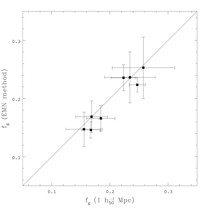
Figure 3.— Gas fractions calculated from usual method ($f_{g}(1h_{50}^{-1}$ Mpc)) and using EMN method to obtain $M_{tot}(r_{500}$) and hence $f_{g}(r_{500}$). Errors shown are 90% confidence limits from temperature measurements.

Figure 4.— $\chi^{2}$ as a function of $q_{0}$. The solid line is the usual method of calculating gas fractions (1 $h_{50}^{-1}$ Mpc) and the dashed line is using the method of EMN ($r_{500}$). The horizontal lines show 95% confidence levels ($\Delta\chi^{2}=3.841$). The best fit for the usual method is $q_{0}$ = 0.07, with 95% confidence limits of -0.47 $<q_{0}<$ 0.67. The EMN method yields a best fit of 0.04 and limits of -0.50 $<q_{0}<$ 0.64.

The low values of $\chi^{2}$ for the best fits above suggest that our error estimates are too conservative. A more robust way of calculating the confidence limits on $q_{0}$ is to use bootstrap resampling (Press et al. 1992). We drew $10^{5}$ artificial data sets from the actual samples for each of our two methods. For the fixed physical radius method, 95% of the calculated values of $q_{0}$ lie between -0.18 and 0.66. For the EMN method, 95% of the calculated values of $q_{0}$ lie between -0.28 and 0.70. These calculations include none of the intrinsic 25% scatter from simulations. If we again assume a maximum 2% actual evolution in the gas fraction, the limits change to $-0.22<q_{0}<0.74$ and $-0.32<q_{0}<0.78$. The agreement with the above results is encouraging, as are the narrower confidence limits.

5. CONCLUSIONS

We have used the apparent change of the cluster gas mass fraction $f_{g}=M_{gas}/M_{tot}$ with redshift together with the assumption of constant true gas fraction to derive constraints on the cosmological deceleration parameter $q_{0}$. Our sample is the first “large” sample of high redshift clusters with a common method of analysis, which is important for an accurate measurement of the apparent change in $f_{g}$ with redshift. We compare high redshift clusters to a similar sample of nearby clusters, namely those with $L_{X}>10^{45}$ erg s^-1, though our results are not strongly affected by this selection. We include the intrinsic 25% scatter in $f_{g}$ predicted by simulations and verified by observations. We obtain $-0.47<q_{0}<0.67$ at 95% confidence using the gas fractions at a constant physical radius of 1 $h_{50}^{-1}$ Mpc and -0.50 $<q_{0}<$ 0.64 with 95% confidence for gas fractions evaluated at a constant overdensity radius. The excellent agreement between these two results suggest that this method to calculate $q_{0}$ is quite promising. Bootstrap resampling yields narrower confidence limits, $-0.18<q_{0}<0.66$ and $-0.28<q_{0}<0.70$ respectively for the two methods. Our results are in good agreement with the upper limit $q_{0}<$0.75 from galaxy counts in redshift surveys (Schuecker et al. 1998) and the lower limit $q_{0}>-2$ from studies of gravitational lensing (Park & Gott 1997).

We find that the standard closed, flat, and open models for the universe are all within the formal 95% confidence limits, as are some flat $\Omega+\Lambda=1$ models with non-zero cosmological constant. We are able to rule out a universe with $\Omega=0$ and $\Lambda=1$. Our results are consistent with observations of high-redshift Type Ia supernovae (Perlmutter et al. 1997, Garnavich et al. 1998, Riess et al. 1998) as well as with gravitational lensing statistics, which yield $\Lambda<0.65$ (Kochanek 1996) at 95% confidence.

Determining $q_{0}$ from distant cluster gas fractions has the significant advantage of being independent of $H_{0}$ and the numerical value of $f_{g}$. Systematic effects could be created by calibration offsets, unknown selection effects, non-Gaussian errors, or cooling flows and mergers which are responsible for much of the intrinsic scatter in the gas fraction. We have included the expected intrinsic scatter in our calculations, and the results of Henry (1997) suggest that calibration offsets between fluxes from Einstein and ASCA are not very significant. The actual cluster gas mass fractions may increase slightly with redshift. This would be true if the gas in nearby clusters has been expelled from the core (e.g., by shock heating) systematically more than in distant clusters. Simulations suggest that this effect is negligible in both $\Omega=1$ and $\Omega<1$ universes. Alternatively, our results would be biased if the local value of $H_{0}$ is significantly different from the global value, although “local” here refers to an average redshift of $z$=0.06. From Figure 2, we can see that the nearby gas mass fraction has much less scatter for “single” clusters (i.e., ones with no significant substructure). Thus, constraints on $q_{0}$ can be greatly improved not just by increasing the sample size but by improving the analysis of individual distant clusters so we can differentiate between clusters with and without substructure and properly measure temperature distributions. In conclusion, although our current results do not improve significantly the determination of $q_{0}$, we have shown that with the assumption of constant gas mass fractions, future detailed X-ray observations with AXAF and XMM can provide useful constraints on $q_{0}$.

REFERENCES

Allen, S.W. et al. 1996, MNRAS, 283, 263

Blumenthal, G.R., Faber, S.M., Primack, J., & Rees, M.J. 1984, Nature, 311, 517

Buote, D.A. & Canizares, C.R. 1996, ApJ, 457, 565

Cavaliere, A. & Fusco-Femiano, R. 1976, A&A, 49, 137

Cooray, A. 1998, A&A, 1998, 333, L71

Danos, R. & Pen, U. 1998, astro-ph/9803058

David, L.P., Arnaud, K.A., Forman, W., & Jones, C. 1990, ApJ, 356, 32

David, L.P., Slyz, A., Jones, C., Forman, W., Vrtilek, S.D., & Arnaud, K.A. 1993, ApJ, 412, 479

David, L.P., Jones, C., & Forman, W. 1995, ApJ, 445, 578

Evrard, A.E. 1997, MNRAS, 292, 289

Evrard, A.E. 1990, in Fitchett, M., Oegerle, W., eds, Clusters of Galaxies. Cambridge Univ. Press, Cambridge, p. 287

Evrard, A.E., Metzler, C.A., & Navarro, J.F. 1996, ApJ, 469, 494

Faber, S.M. & Gallagher, J.S. 1976, ApJ, 204, 365

Forman, W. & Jones, C. 1982, ARA&A, 20, 547

Frenk, C.S. et al. 1998, “The Santa Barbara Cluster Comparison Project”, in preparation.

Garnavich, P.M. et al. 1998, ApJ, 493, L53

Henry, J.P. 1997, ApJ, 489, L1

Henry, J.P. & Briel, U.G. 1995, ApJ, 443, L9

Henry, J.P. & Tucker, W. 1979, ApJ, 229, 78

Jones, C. & Forman, W. 1984, ApJ, 276, 38

Jones, C. & Forman, W. 1998, accepted.

Kang, H., Cen, R., Ostriker, J.P., & Ryu, D. 1994, ApJ, 428, 1

Katz, N., Hernquist, L., & Weinberg, D.H. 1992 ApJ, 399, 109

Kochanek, C.S. 1996, ApJ, 466, 638

Lubin, L.M., Cen, R., Bahcall, N., & Ostriker, J.P. 1996, ApJ, 460, 10

Markevitch, M. & Vikhlinin, A. 1997, ApJ, 491, 467

Markevitch, M., Forman, W.R., Sarazin, C.L., & Vikhlinin, A. 1997, astro-ph/9711289

Mushotzky, R.F. & Loewenstein, M. 1997, ApJ, 481, L63

Mushotzky, R.F. & Scharf, C.A. 1997, ApJ, 482, L13

Navarro, J.F., Frenk, C.S., & White, S.D.M. 1995, MNRAS, 275, 720

Neumann, D.M. & Böhringer, H. 1997, MNRAS, 289, 123

Park, M. & Gott, J.R. 1997, ApJ, 489, 476

Pen, U. 1998, ApJS, 115, 19

Pen, U. 1997, New Astronomy, 2, 4, 309

Perlmutter, S. et al. 1997, ApJ, 483, 565

Press, W.H., Teukolsky, S.A., Vetterling, W.T., & Flannery, B.P. 1992, Numerical Recipes in FORTRAN, 2nd ed. Cambridge Univ. Press, Cambridge

Riess, A.G. et al. 1998, astro-ph/9805201

Rines, K. et al. 1998, in preparation.

Sandage, A.R. 1988, ARA&A, 26, 561

Sasaki, S. 1996, PASJ, 48, L119

Schindler, S. & Wambsganss, J. 1996, A&A, 313, 113

Schuecker et al. 1998, ApJ, 496, 635

Thomas, P.A. & Couchman, H.M.P. 1992, MNRAS, 257, 11

White, S.D.M., Navarro, J.F., Evrard, A.E., & Frenk, C.S. 1993, Nature, 366, 429

Zombeck, M.V. 1990, Handbook of Space Astronomy and Astrophysics, 2nd ed. Cambridge Univ. Press, Cambridge