The GOSSIP on the MCV V347 Pav.

Abstract

Modelling of the polarized cyclotron emission from magnetic cataclysmic variables (MCVs) has been a powerful technique for determining the structure of the accretion zones on the white dwarf. Until now, this has been achieved by constructing emission regions (for example arcs and spots) put in by hand, in order to recover the polarized emission. These models were all inferred indirectly from arguments based on polarization and X–ray light curves.

Potter, Hakala & Cropper (1998) presented a technique (Stokes imaging) which objectively and analytically models the polarized emission to recover the structure of the cyclotron emission region(s) in MCVs. We demonstrate this technique with the aid of a test case, then we apply the technique to polarimetric observations of the AM Her system V347 Pav. As the system parameters of V347 Pav (for example its inclination) have not been well determined, we describe an extension to the Stokes imaging technique which also searches the system parameter space (GOSSIP).

1 Introduction

Many authors (e.g. Potter et al. 1997; Wickramasinghe & Ferrario 1988; Beuermann, Stella & Patterson 1987; Cropper 1986) have found that the emission region in MCVs must be extended into an arc or comma shape in order to explain the shape of the polarized cyclotron light curves. Until now, the parameters that define the shape and location of the emission regions have been adjusted by a trial-and-error approach until the model gave a good fit. Clearly the number of free parameters describing the location, shape and structure of the emission regions becomes very large.

The technique of Potter, Hakala & Cropper (1998, PHC) objectively modelled the polarimetric data and obtained maps of the emission regions for the first time. Their model had the anisotropies of polarized emission incorporated into it. This allowed them to model the intensity, circular polarization, linear polarization and position angle data. Instead of using the maximum-entropy method and the conjugate optimization (used on intensity data of Cropper & Horne 1994) they used Tikhonov regularization and a genetic algorithm for optimisation.

1.1 The cyclotron model

The first step in modelling cyclotron emission from MCVs is to calculate the viewing angle, i.e., the angle between the line of sight and the magnetic field line from where the emission emanates. This was done by using a dipole magnetic field formalism for the white dwarf, together with a system inclination and offset dipole parameters (see Cropper 1989). For a given magnetic longitude and latitude of the emission point on the white dwarf, the viewing angle was obtained for different phases of the spin cycle. The local magnetic field was calculated and subsequently the local optical depth parameter. The intensity spectrum and percentage of circular and linear polarization was then calculated from interpolating on the cyclotron opacity calculations of Wickramasinghe and Meggitt (1985). Extended sources were modelled by summing the components of many such emission points as a function of spin phase.

The optimisation of the model to the data proceeds by adjusting the number and distribution of emission points across the surface of the white dwarf. During the optimisation the inclination, magnetic dipole offset (in latitude and azimuth) and the magnetic field strength at the poles are kept fixed.

1.2 Stokes Imaging

PHC used a genetic algorithm (GA) in order to optimise the fit to the data. The GA works by first generating a set of random solutions. The fitness of each solution is then calculated using

$$F(p)=\chi^{2}+\lambda\sum_{i}{\|\nabla p_{i}\|^{2}}$$ (1)

where $\|\nabla p_{i}\|$ is the mean gradient of the number of emission points at point i and $\chi^{2}$ is the chi-square fit. The fitness is a measure of how good the fit is to the data plus the smoothness of the image solution. The solutions are ranked in order of their fitness. The next generation of solutions are then produced by a type of natural selection procedure – the solutions that were ranked best are more probable to breed the next generation and the next population is generated by applying genetic crossover and mutation operators to the selected parent pairs.

Eventually, after many generations, the improvement in fitness of the GA solutions will start to level out and a more analytical approach is required to improve the fit further. For the final approach to minimum the Powell’s method line minimisation routine (see Press et al. 1992) was used.

1.3 The test case

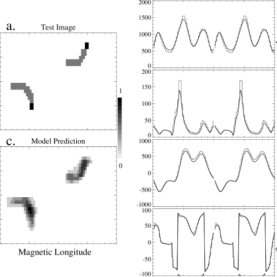
Figure 1: The test case a. The emission on the surface of the white dwarf. b. The test emission light curves (histogram) and the model fit (solid smooth curve). c. The optimised image.

To demonstrate the technique we have generated synthetic Stokes parameter curves with 50 points over the orbital phase (typical datasets have roughly this number). This gives us 200 data points to fit. In this paper we use a 6 degree resolution map on the white dwarf surface, which in turn yields 1740 free parameters ($60\times 29$ surface grid elements on the white dwarf surface). The simulated polarized light curves presented below were produced by calculating the emission that would arise from two extended sources (Fig. 1a) in the B–band. The resulting light curves (Fig. 1b) has infinite signal–to–noise ratio. The inclination was $80^{\rm o}$, the magnetic dipole offset was $10^{\rm o}$, the magnetic polar field strength was $60$ MG and the polar optical depth parameter $\Lambda$ was $1.0\times 10^{5}$.

Figure 1b shows the model fit (thick smooth curves) to the input test data (histogram curves). The optimisation technique has reproduced the complex features arising from the extended regions. These include the linear and intensity features such as dips and peaks. It has also correctly modelled both the positive and negative polarized light curves.

Figure 1c shows the model prediction for the shape and location of the emission regions. The grey scale is a measure of the optical depth across the emission region. As can be seen from the figure, the optimisation routine has accurately located and mapped the emission regions across the surface of the white dwarf.

2 Genetically Optimised ‘Super’ Stokes Imaging Procedure (GOSSIP)

For the test case described above we created polarimetric light curves using the cyclotron model. Therefore, the system parameters (inclination, magnetic field orientation and strength) were known. In the case of real data these parameters are generally unknown.

PHC explained that the system parameters were not included in the optimisation procedure. This is because these parameters are qualitatively different from those describing each point on the derived map. Therefore, the system parameter space has to be searched separately from that searched during the ‘Stokes imaging’ technique, either by trial and error, or by the use of a genetic algorithm operating as an outer loop to the ‘Stokes imaging’ procedure. The outer optimisation loop optimises the final fitness values produced by several optimised solutions. In effect, the optimised solutions produced by several runs of the ‘Stokes imaging’ technique become solutions for genetic optimisation themselves.

2.1 The MCV V347 Pav

Figure 2: The ‘Stokes imaging’ solution to the polarimetric observations of Ramsay et al. (1996) for an inclination $=62^{\rm o}$ and a dipole offset $=36^{\rm o}$. a. The blue data. b. The red data.

Figure 2a,b shows the blue and red polarimetric observations of the MCV V347 Pav (RE J1844-741) from Ramsay et al (1996). Bailey et al (1995) suggested that the positive and negative excursions of the circular polarization over the orbital period of $\sim$ 90 mins was due to emission arising from two regions located at or near opposite ends of the magnetic field. The high signal-to-noise observations of Ramsay et al. (1996) make them ideal for the optimisation technique.

The technique predicts a best fit for an inclination of $62^{\rm o}$, dipole offset of $32^{\rm o}$ and magnetic field strengths of 28 and 24MG for the upper and lower poles respectively. From Figure 2 it can be seen that the optimised model solution has reproduced the red polarization data remarkably well. The morphology of all the red polarized light curves has been accurately predicted, in particular, the variation in position angle, the relative amounts of linear and circular flux, the peaks and dips in the circular polarization and the overall variation in the intensity curve. It has also predicted the gross features of the blue polarized variations and the correct amount of relative flux between the two wave bands. The technique finds a solution that fits both wave bands simultaneously.

However, it has not modelled the finer details of the blue polarimetric variations. This has arisen because of the less accurate determination for the magnetic field strengths, thus affecting the quality of the fit to one wave-band more than the other (the relative fluxes between the two wave-bands depends on the magnetic field strength). Also, the red polarimetric observations have significantly more counts than the blue band. Therefore, the optimisation routine will be more biased towards fitting the red data. The fit to the blue data can be improved by increasing the magnetic field strength on the upper pole. Maintaining a dipole field constraint, however, makes the fit to the red data significantly worse. Any temperature structure within the shock will also affect the finer details of the polarized light curves in different bands. We have assumed a constant temperature of 10keV for the emitting gas.

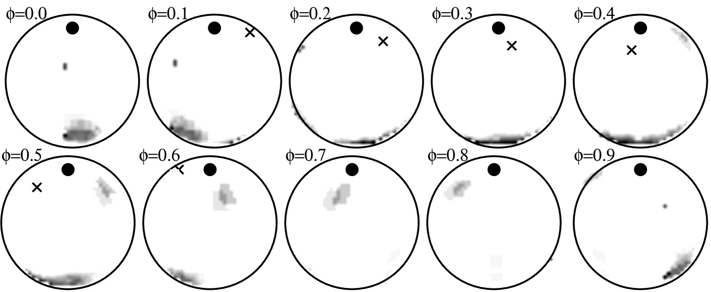
Figure 3: The position of the cyclotron emission regions as viewed from Earth for a complete orbital rotation. The dot and the cross represent the spin and magnetic poles respectively.

Figure 3 shows the predicted emission regions mapped onto a sphere representing the surface of the white dwarf as viewed from Earth for a complete orbital rotation. The observed features of the polarimetric observations (Figure 2a,b) can be explained with reference to Figure 3. The most prominent feature of the observations is the bright and faint phase. The main emission region in the lower hemisphere is responsible for the bright phase emission during $\phi\sim 0.0$–$0.5$ and the secondary smaller emission region is responsible for the faint phase emission during $\phi\sim 0.5$–$1.0$. The south west–north east orientation of the main emission region means that it gradually appears over the limb of the white dwarf at $\phi\sim 0.0$ and then rapidly disappears at $\phi\sim 0.5$ resulting in a large linearly polarized pulse. The secondary emission region is visible for a larger fraction of the orbital period. It first appears just before $\phi\sim 0.4$ and therefore contributes to the large linearly polarized pulse. At $\phi\sim 0.8$ the magnetic field lines feeding the secondary emission region are most pointing towards the line of sight resulting in depolarization of the radiation by cyclotron self-absorption. This is evident from the dip in the positive circular polarization. The secondary region then moves away from the line of sight, resulting in an increase in emission (seen as the contribution to the rapid increase in the intensity) and the brief increase in positive circular polarization at $\phi\sim 1.0$ . The secondary emission region continues to stay on the upper limb of the white dwarf and gives rise to the linear pulse at phase $\sim 0.2$ . The more gradual decline in the intensity from the bright phase at $\phi\sim 0.5$ (seen especially in IR observations in Bailey et al. 1995) can be attributed to the presence of the secondary region.

2.2 The accretion region

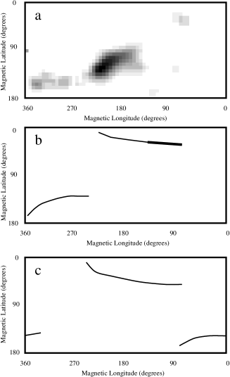
Figure 4: A comparison between: a. The optimised image solution. b. The model prediction in Ramsay et al. (1996) c. The model prediction of Bailey et al. (1995).

In Figure 4 we compare our prediction for the shape and location of the cyclotron emission region with that of previous work. The figures are mapped onto a flat surface. As a result, the large differences in longitude near the polar regions are much smaller on the surface of a sphere than they appear on the maps. The emission region is mapped onto the same coordinate system used in each case. Figure 4b shows the prediction for the shape and location of the emission region from Ramsay et al. (1996). The main difference is that Ramsay et al. (1996) located the main emission region responsible for the negative polarization on the upper hemisphere of the white dwarf. They also used a much higher value for the inclination ($80^{\rm o}$) as an explanation for the equal orbital coverage of the bright and faint phases and the variation in the position angle. Furthermore, they used two long thin arcs. The only similarity is that both models predict enhanced brightness on the trailing edge of the main emission region.

Figure 4c shows the model prediction of Bailey et al. (1995). They also predicted two long thin arcs located in approximately the same locations (large changes in magnetic longitude near the poles, translate to small changes in actual position) as that of Ramsay et al. (1996). However, they locate the main emission region in the lower hemisphere in agreement with the ‘Stokes imaging’ technique. Furthermore, Bailey et al. (1995) estimated an orbital inclination of $i=60^{\rm o}$ and a magnetic dipole offset of $\beta=50^{\rm o}$, also in closer agreement with the ‘Stokes imaging’ technique.

3 Summary

In this paper we have applied an extension of the Stokes imaging technique, developed and discussed in PHC, simultaneously to the blue (3500–6500Å ) and red (5500–9500Å ) polarimetric observations of the AM Her star V347 Pav from Ramsay et al. (1996). We have also described an extension to the Stokes imaging technique, which also searches the system parameter space.

Our technique has predicted an extended main cyclotron emission region, located in the lower hemisphere of the white dwarf, and a secondary, smaller less dense region diametrically opposite. The main emission region is found to consist of a higher density region whose center is located $\sim 25^{\rm o}$ from the magnetic equator. It has a broken extended region extending ahead in phase towards but trailing the magnetic pole. The technique also predicts a secondary emission region in the upper hemisphere which is relatively less dense than the main emission region. It is smaller in extent and almost diametrically opposed to the center of the main emission region. These maps are different from those from previous less objective techniques in which two long thin arcs were used to reproduce the polarimetric variations.

- [1] ailey, J. A. et al., 1995, MNRAS, 272, 579
- [2] euermann, K., Stella, L. & Patterson, J., 1987 ApJ, 316, 360
- [3] ropper, M. S., 1989, MNRAS, 236, 935
- [4] ropper, M, & Horne, K. 1994, MNRAS, 267, 481
- [5] otter, S. B., Cropper, M, Mason, K. O., Hough, J. H. & Bailey, J. A., 1997, MNRAS, 285, 82
- [6] otter, S. B., Hakala, P. J. & Cropper, M, (PHC) 1998, MNRAS297, 1261
- [7] ress, W. H., Teukolsky, S. A., Vetterling W.T. & Flannery, B. P., 1992, Numerical Recipes in FORTRAN, Cambridge University Press, p406
- [8] amsay, G., Cropper, M., Wu, K. & Potter, S., 1996, MNRAS, 282, 726
- [9] ickramasinghe, D. T., & Ferrario, L., 1988 ApJ, 334, 412
- [10] ickramasinghe, D. T., & Meggitt, S. M. A., 1985, MNRAS, 214, 605
- [11]