Ring diagram analysis of near-surface flows in the Sun

Abstract

Ring diagram analysis of solar oscillation power spectra obtained from MDI data is carried out to study the velocity fields in the outer part of the solar convection zone. The three dimensional power spectra are fitted to a model which has a Lorentzian profile in frequency and which includes the advection of the wave front by horizontal flows, to obtain the two components of the sub-surface flows as a function of the horizontal wave number and radial order of the oscillation modes. This information is then inverted using OLA and RLS methods to infer the variation in horizontal flow velocity with depth. The average rotation velocity at different latitudes obtained by this technique agrees reasonably with helioseismic estimates made using frequency splitting data. The shear layer just below the solar surface appears to consist of two parts with the outer part up to a depth of 4 Mm, where the velocity gradient does not show any reversal up to a latitude of $60^{\circ}$. In the deeper part the velocity gradient shows reversal in sign around a latitude of $55^{\circ}$. The zonal flow velocities inferred in the outermost layers appears to be similar to those obtained by other measurements. A meridional flow from equator polewards is found. It has a maximum amplitude of about 30 m/s near the surface and the amplitude is nearly constant in the outer shear layer.

1 Introduction

The rotation rate in the solar interior has been inferred using the frequency splittings for p-modes (Thompson et al. 1996; Schou et al. 1998). However, the splitting coefficients of the global p-modes are sensitive only to the north-south axisymmetric component of rotation rate. To study the non-axisymmetric component of rotation rate and the meridional component of flow, other techniques based on ‘local’ modes are required. Since these velocity components are comparatively small in magnitude they have not been measured very reliably even at the solar surface. The primary difficulty in measuring meridional flow velocities at solar surface arises from convective blue shifts due to unresolved granular flows (Hathaway 1987, 1992). Additional difficulty is caused by the fact that at low latitudes the line of sight component of meridional velocity is small. Sunspots and other magnetic features have also been used to measure meridional flow (Howard 1996). There is a considerable difference in the results of these measurements. Using direct Doppler measurements at the solar surface from GONG instruments Hathaway et al. (1996) have measured various components of nearly steady flows on the solar surface. They find a polewards meridional flow with an amplitude of about 27 m/s, which varies with time. There is also some evidence for north-south difference in the rotation rate (Antonucci, Hoeksema & Scherrer 1990; Verma 1993; Carbonell, Oliver & Ballester 1993; Hathaway et al. 1996) but once again there is no agreement on the magnitude of this component or its statistical significance.

Apart from these nearly steady flows, there could also be cellular flows with very large length scales and life-times, viz., the giant cells. However, there has been no firm evidence for such cells (Snodgrass & Howard 1984; Durney et al. 1985), though recently Beck, Duvall & Scherrer (1998) have reported probable detection of giant cells from the analysis of Michelson Doppler Imager (MDI) Dopplergrams. These large scale flows are believed to play an important role in transporting magnetic flux and angular momentum and thus, their study is important for understanding the theories of solar dynamo and turbulent compressible convection (Choudhuri, Schussler & Dikpati 1995; Brummell, Hurlburt & Toomre 1998; Rekowski & Rüdiger 1998).

High-degree solar modes ($\ell\gtrsim 150$) which are trapped in the solar envelope have lifetimes that are much smaller than the sound travel time around the Sun and hence the characteristics of these modes are mainly determined by average conditions in local neighborhood rather than the average conditions over the entire spherical shell. These modes can be employed to study large scale flows inside the Sun, using time-distance analysis (Duvall et al. 1993, 1997; Giles et al. 1997), ring diagrams (Hill 1988; Patrón et al. 1997) and other techniques. Using time-distance helioseismology Giles et al. (1997) have studied the meridional flow to find that the meridional velocity does not change significantly with depth, while Schou & Bogart (1998) using the ring diagram technique find some increase in meridional velocity with depth. Ring diagram analysis of meridional flows have also been done by González Hernández et al. (1998a) and Basu, Antia & Tripathy (1998), who also find some variation in meridional flow with depth. Haber et al. (1998) find that the velocity of the surface flows can change over moderately short time scales. González Hernández et al. (1998b) have demonstrated the reliability of ring diagram analysis by comparing results obtained from data collected simultaneously by two independent instruments, namely, the MDI and one of the Taiwan Oscillation Network (TON) instrument at Observatorio del Teide.

Ring diagram analysis is based on the study of three-dimensional (henceforth 3d) power spectra of solar p-modes on a part of the solar surface. If one considers a section of a 3d spectrum at fixed temporal frequency, one finds that power is concentrated along a series of rings that correspond to different values of the radial harmonic number $n$. The frequencies of these modes are affected by horizontal flow fields suitably averaged over the region under consideration, hence, an accurate measurement of these frequencies will contain the signature of large scale flows and can be used to study these flows. The measured frequency shifts for different modes can be inverted to obtain the horizontal flow velocities as a function of depth. The local nature of these modes allows us to study different regions on the solar surface, thus giving a three dimensional information about the horizontal flows. Since the high degree modes used in these studies are trapped in the outermost layers of the Sun, such analysis gives information about the conditions in the outer 2–3% of the solar radius.

In this work we use ring diagram analysis to study the longitudinal as well as latitudinal component of horizontal velocity in the outer layers of the Sun. Although, it is possible to study the variation in horizontal velocity with both longitude and latitude, in this work we have only considered the longitudinal averages, which contains information about the latitudinal variation in these flows. For this purpose, at each latitude we have summed the spectra obtained for different longitudes to get an average spectrum which has information on the average flow velocity at each latitude. The longitudinal velocity component is dominated by the rotation velocity and can be used to study its variation with depth and latitude. This complements the results obtained from the inversion of frequency splittings of global p-modes. Since the splittings of global p-modes are not reliably determined at high degree these inversions are not very reliable in regions close to surface. It should, however, be possible to determine the rotation rate in this region more reliably with ring diagram analysis using data that include high degree modes extending up to $\ell\approx 1200$. In particular, the shear layer just below the solar surface can be examined in more detail. Besides, ring diagram analysis also enables us to measure the north-south variation in the rotation rate at same latitude. The latitudinal component of velocity is dominated by the meridional flow and can be used to study its variation with latitude and depth. This work uses a larger data set covering an entire solar rotation period and has improved fits as compared to the work reported in Basu et al. (1998). We have also included an improved analysis of the meridional flow results and identified higher order terms in this flow.

The rest of the paper is organized as follows: Section 2 describes the basic technique used to calculate the horizontal flow velocities using ring diagrams. Section 3 describes the results, while Section 4 gives the conclusions from our study.

2 The technique

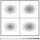
Figure 1: Sample (logarithmic) power spectra as a function of $k_{x}$ and $k_{y}$ at a fixed frequency. The top panels are for the average spectrum centered at equator, at frequencies of around 3 mHz (left) and 4 mHz (right). The bottom panels are for the spectrum centered at $45^{\circ}$N latitude, at frequencies of around 3 mHz (left) and 4 mHz (right). The scale is marked with the logarithm of the power.

A good description of the ring diagram technique can be found in Hill (1988, 1994) and Patrón et al. (1997). We, therefore, only outline the procedure used by us in this work. We have used data from full-disk Dopplergrams obtained by the MDI instrument of the Solar Oscillations Investigation (SOI) on board SoHO. Selected regions of Dopplergrams mapped with Postel’s projection are tracked at a rate corresponding to the photospheric rotation rate (Snodgrass 1984) at the center of each region to filter out the photospheric rotation velocity from the flow fields. This allows us to study the smaller components of the flow which are not very well determined from other studies. Since the solar rotation rate generally increases with depth just below the surface, the increase in rotation velocity will contribute to the longitudinal component of horizontal flows measured by the ring diagram technique. For each tracked region, the images are detrended by subtracting the running mean over 21 neighboring images to filter the series temporally. Detrending eliminates slowly varying signals such as those from local activity and nearly steady flows. The detrended images are apodized and Fourier transformed in the two spatial coordinates and in time to obtain the 3d power spectra. We have chosen the spatial extent of the region to be about $15^{\circ}\times 15^{\circ}$ with $128\times 128$ pixels in heliographic longitude and latitude giving a resolution of $0.03367$ Mm^-1 or 23.437 $R_{\odot}^{-1}$. Each region is tracked for 4096 minutes giving a frequency resolution of 4.07 $\mu$Hz. To minimize effects of foreshortening all the regions were centered on the central meridian, however, the high latitude regions will still suffer from foreshortening. Near the equator, each such region covers an area of roughly $182\times 182$ Mm on the solar surface and hence will include a few supergranules. There may still be some contribution from supergranular velocities in the average flow over each region, which will interfere with the signal from nearly steady and large scale flows. Since in this work we are considering only averages over all longitudes there will be further averaging of the supergranular flows and their contribution is expected to be very small. The spectra have been obtained using the relevant tasks in MDI data-processing pipeline. Fig. 1 shows a few sections of some of these spectra at constant frequency.

We have selected the regions centered at Carrington longitudes of $90^{\circ},60^{\circ},30^{\circ}$ for Carrington rotation 1909 and at $360^{\circ},330^{\circ},300^{\circ}$, $275^{\circ}$, $235^{\circ}$, $210^{\circ}$, $183^{\circ}$, $143^{\circ}$, and $120^{\circ}$ for rotation 1910 corresponding to a period from about May 24 to June 21, 1996, covering an entire Carrington rotation period. The uneven distribution of longitudes was dictated by the need to avoid, as far as possible, large gaps in the data. For each longitude we select regions centered at latitudes of $60^{\circ}$ south to $60^{\circ}$ north at steps of $5^{\circ}$. Thus there is some overlap between different regions. Since in this work we are only interested in latitudinal variation in the flow fields, we take a sum of all spectra for a given latitude which gives us a spectrum averaged over all longitudes. Because of averaging, these spectra have better statistics and the error estimates are also lower.

To extract the flow velocities and other mode parameters from the 3d power spectra we fit a model of the form

$$P(k_{x},k_{y},\nu)={\exp(A_{0}+(k-k_{0})A_{1}+A_{2}({k_{x}\over k})^{2}+A_{3}{k_{x}k_{y}\over k^{2}})\over(\nu-ck^{p}-U_{x}k_{x}-U_{y}k_{y})^{2}+(w_{0}+w_{1}(k-k_{0}))^{2}}+{e^{B_{1}}\over k^{3}}+{e^{B_{2}}\over k^{4}}$$ (1)

where $k^{2}=k_{x}^{2}+k_{y}^{2}$, $k$ being the total wave number, and the 12 parameters $A_{0},A_{1},A_{2},A_{3},c,p,U_{x},U_{y},w_{0},w_{1},B_{1}$ and $B_{2}$ are determined by fitting the spectra using a maximum likelihood approach (Anderson, Duvall & Jefferies 1990). Here $k_{0}$ is the central value of $k$ in the fitting interval. The mean power in the ring is given by $\exp(A_{0})/w_{0}^{2}$. The coefficient $A_{1}$ accounts for the variation in power with $k$ in the fitting interval. Only the linear term is included as the fitting interval is generally quite small. The $A_{2}$ and $A_{3}$ terms account for the variation of power along the ring, namely, the variation with direction of propagation of the wave. These were introduced because the power does appear to vary along the ring and the fits in the absence of these terms were not satisfactory. This variation can be easily seen in the outermost ring in the power spectra displayed in Fig. 1. The outermost ring in the spectra around 3 mHz is for $n=0$, while for spectra around 4 mHz the outermost ring is for $n=1$ as the $n=0$ ring will be around $\ell=1600$, which is beyond the range of our spectra. The variation in power along the ring may be due to foreshortening or other systematic effects and may not represent a real variation in the power spectrum of the Sun. The term $ck^{p}$ gives the mean frequency and this form is chosen as it gives satisfactory fits to the mean frequency over the whole fitting interval. The terms $U_{x}k_{x}$ and $U_{y}k_{y}$ represent the shift in frequency due to large scale flows and the fitted values of $U_{x}$ and $U_{y}$ give the average flow velocity over the region covered by the power spectrum and the depth range where the corresponding mode is trapped. The mean half-width is given by $w_{0}$, while $w_{1}$ takes care of the variation in half-width with $k$ in the fitting interval. The terms involving $B_{1},B_{2}$ define the background power, which is assumed to be of the same form as Patrón et al. (1997). The fitting formula given by Eq. (1) is slightly different from what is used by Patrón et al. (1997), in that we have assumed some variation in amplitude along the ring (given by the $A_{2}$ and $A_{3}$ terms), and we also include variation in power and width with $k$ through the coefficients $A_{1}$ and $w_{1}$. Basu et al. (1998) did not include the $w_{1}$ term and the background terms used by them were also slightly different. Here, the positive $x$ direction is the direction of solar rotation and the positive $y$ direction is towards the north in heliographic coordinates.

The fits are obtained by maximizing the likelihood function $L$ or minimizing the function $F$

$$F=-\ln L=\sum_{i}\left(\ln M_{i}+{O_{i}\over M_{i}}\right),$$ (2)

where summation is taken over each pixel in the fitting interval. The term $M_{i}$ is the result of evaluating the model given by Eq. (1) at $i^{\rm th}$ pixel defined by $k_{x},k_{y},\nu$ in the 3d power spectrum, and $O_{i}$ is the observed power at the same pixel. The minimization has been performed using a quasi-Newton method based on the BFGS (Broyden, Fletcher, Goldfarb and Shanno) formula for updating the Hessian matrix (Antia 1991). The error bars are obtained from the inverse of the Hessian matrix at the minimum (Anderson et al. 1990).

In order to test the sensitivity of fits to the form of fitted function, we have repeated the fits with some parameters kept fixed. For example, we have tried fits keeping $w_{1}=0$ or $A_{2}=A_{3}=0$ and also some fits where $w_{0}$ is kept fixed at the initial guess. For background terms we have also tried exponents other than what are included in Eq. (1). We have also attempted fits with more parameters including variation in power due to higher order terms in $k_{x},k_{y}$. From these experiments we find that the fitted values of $U_{x}$ and $U_{y}$ are fairly robust to these changes and the differences between different fits are less than the estimated errors. The form given by Eq. (1) was chosen because all the parameters appearing there have significant values in some region and the fit appears to be satisfactory. While additional parameters which were tried generally turned out to be small and comparable to the corresponding error estimates. To evaluate the quality of the fit we use the merit function (cf., Anderson et al. 1990)

$$F_{m}=\sum_{i}\left(O_{i}-M_{i}\over M_{i}\right)^{2}$$ (3)

where the summation is over all pixels in the fitting interval and $O_{i}$ and $M_{i}$ are as defined in Eq. (2). We find that with the choice of model given by Eq. (1), the merit function comes out to be close to unity in all successful fits. If some of the parameters in Eq. (1) are kept fixed then the merit function increases. On the other hand, adding more parameters does not reduce the merit function significantly.

We fit each ring separately by using the portion of power spectrum extending halfway to the adjoining rings. For each fit a region extending about $\pm 100\mu$Hz from the chosen central frequency is used. We choose the central frequency for fit in the range of 2–5 mHz as the power outside this range is not significant. The rings corresponding to $0\leq n\leq 6$ have been fitted. For each value of $n$ we increase the central frequency of the fitting interval in steps of 12.21 $\mu$Hz or 3 pixels in the spectra. This gives us typically 800 ‘modes’, all of which may not be independent as there is a considerable overlap between adjacent fitting intervals. In this work we express $k$ in units of $R_{\odot}^{-1}$, which enables us to identify it with the degree $\ell$ of the spherical harmonic of the corresponding global mode.

The fitted $U_{x}$ and $U_{y}$ for each mode represents an average — over the entire region in horizontal extent and over the vertical region where the mode is trapped — of the velocities in the $x$ and $y$ directions respectively. We can invert the fitted $U_{x}$ (or $U_{y}$) to infer the variation in horizontal flow velocity $u_{x}$ (or $u_{y}$) with depth. We use the Regularized Least Squares (RLS) as well as the Optimally Localized Averages (OLA) (Backus & Gilbert 1968) techniques for inversion. The results obtained by these two independent inversion techniques are compared to test the reliability of inversion results.

In the RLS method we try to fit $U_{x}$ (or $U_{y}$) under the constraint that the underlying $u_{x}$ (or $u_{y}$) is smooth. We represent $u_{x}$ (or $u_{y}$) in terms of a cubic B-Spline basis and the coefficients are determined by $\chi^{2}$ minimization with first derivative regularization.

In the OLA technique the aim is to explicitly form linear combinations of the data and the corresponding kernels such that the resulting averaging kernels are as far as possible localized near the position for which the solution is being sought. This is done by minimizing

$$\int(r-r_{0})^{2}\left(\sum_{i}c_{i}K_{i}\right)^{2}dr+\mu\sum_{i}c^{2}_{i}\sigma^{2}_{i},$$ (4)

where $K_{i}$ are the mode kernels, $\mu$ is a trade-off parameter that ensures that the propagated errors in the solution are low. The minimization is done subject to the condition that the averaging kernel, defined as ${\cal K}(r)=\sum_{i}c_{i}K_{i}(r)$, is unimodular, i.e., $\int{\cal K}(r)dr=1$.

For the purpose of inversion, the fitted values of $U_{x}$ and $U_{y}$ are interpolated to the nearest integral value of $k$ (in units of $R_{\odot}^{-1}$) and then the kernels computed from a full solar model with corresponding value of degree $\ell$ are used for inversion. Since the fitted modes are trapped in outer region of the Sun, inversions are carried out for $r>0.97R_{\odot}$ only.

3 Results

Following the procedure outlined in Section 2 we fit the form given by Eq. (1) to a suitable region of a 3d spectrum. Fig. 2 shows some of the fitted quantities for the averaged spectrum centered at the equator. The error bars are not shown for clarity. The power is maximum around a frequency of 3 mHz for modes with $n>1$. The fitted half-width $w_{0}$ appears to increase at low frequencies. This increase is probably artificial and we have checked that keeping the width fixed during the fit for these modes does not affect the fitted $U_{x}$ and $U_{y}$. Although not shown, we find that the parameters $A_{1},A_{2},A_{3}$ defining the variation in power with $k,k_{x},k_{y}$ all have significant values. The parameters $A_{2}$ and $A_{3}$ increase significantly with $k$ and this can be seen from the power spectra shown in Fig. 1, where the variation of power along the ring is clearly visible in the outer rings. In general only one of the two background terms defined by $B_{1}$ and $B_{2}$ is significant, with $B_{2}$ being the more dominant at higher $\ell$. It thus appears that the background decreases more rapidly with $\ell$ at higher $\ell$. In principle, the mean frequency $\nu_{0}=ck^{p}$ can also be computed from the fits, but there would be some systematic errors in these values, as in other ridge fitting techniques (Bachmann et al. 1995). The exponent $p$ varies between 0.35 to 0.55 for various modes. For f-modes it is in general very close to 0.5 which is the expected asymptotic value for a standard solar model.

Although other quantities may also be of some interest, in this work we restrict our attention to the two horizontal components of velocity obtained by fitting the spectra. These are shown in Fig. 3 for various latitudes. From this figure it appears that $U_{x}$ generally increases with depth, except possibly at high latitudes. On an average, $U_{x}$ appears to be lower at high latitudes, mainly due to the $\cos(\theta)$ (where $\theta$ is the latitude) factor in conversion from angular velocity to linear velocity. The latitudinal component $U_{y}$ is positive in the northern hemisphere and negative in the southern hemisphere and thus the meridional flow is directed from equator to poles. Further, the meridional component appears to be comparatively independent of depth at low latitudes, while at high latitudes there is some variation with depth. The fitted velocities for each ‘mode’ are inverted to obtain the variation of horizontal velocity with depth. Only the region $r>0.96R_{\odot}$ is sampled by the modes used in this study and hence the inversions are restricted to $r>0.97R_{\odot}$ as below this depth the averaging kernels are not properly localized. A sample of the averaging kernels for OLA inversion are shown in Fig. 4. Note that by $r=0.97R_{\odot}$, the averaging kernels become wide and thus have poor resolution. Also note that the peak of the averaging kernel for 0.9987$R_{\odot}$ is shifted slightly inwards, this is because there are very few modes in the data set with turning points in that region.

3.1 The rotation velocity

From the inversion results it appears that the longitudinal component ($u_{x}$) is dominated by the average rotational velocity. This is due to the fact that tracking is done at the surface rotation rate at the center of the tracked region and hence does not account for the variation of the rotation rate with depth. This velocity can be compared with the helioseismic estimate after subtracting out the surface velocity used in tracking. We find that there is a reasonable agreement between $u_{x}$ and the rotation rate determined from splitting coefficients of the global p-modes. Thus, this provides a test of our procedure for inferring the subsurface velocity components. The results obtained using the RLS and OLA techniques for inversion also agree with each other to within the estimated errors.

The rotation velocity at each latitude can be decomposed into the symmetric part [$(u_{N}+u_{S})/2$] and an antisymmetric part [$(u_{N}-u_{S})/2$]. The symmetric part can be compared with the rotation velocity as inferred from the splittings of global modes (Basu & Antia 1998) which sample just the symmetric part of the flow. The comparison is shown in Fig. 5. Since the inversion results using global modes which are restricted to a mode-set of $\ell\leq 250$ are not particularly reliable in the surface regions, the velocity profiles obtained from the ring diagram analysis supplement those results and support the earlier conclusions.

The shear layer just below the surface where the rotation rate increases with depth has been seen in inversion results from global p-modes (Schou et al. 1998; Antia, Basu & Chitre 1998). Some of these inversion results show a change of sign in the velocity gradient just below the solar surface at high latitudes. It would be interesting to study this shear layer using ring diagram analysis. From the results shown in Fig. 5, it appears that the there is some tendency for reversal of gradient near the surface at high latitudes. This tendency for reversal is probably not significant since this feature is seen in the region $r\gtrsim 0.998R_{\odot}$, and at these high latitudes there are very few modes with lower turning points in this region (cf., Fig. 3) making the inversion results less reliable. To some degree this feature is seen at all latitudes. At lower latitudes the extent is somewhat less, which supports the view that this is due to lack of modes with lower turning point in the outermost region. Spectra from high resolution Dopplergrams will help in the study of this region. Leaving aside this region, it appears that the shear layer actually consists of two layers, in the outer layer ($r\gtrsim 0.994R_{\odot}$ or depth $\lesssim 4$ Mm) the gradient is in general quite steep and continues till the latitude of $60^{\circ}$. While in the second layer below this depth the gradient is smaller and appears to reverse its sign around $55^{\circ}$ latitude. The results obtained from global p-modes from MDI data shows a reversal in the sign of the gradient at latitudes of $55^{\circ}$. It is possible that this is due to relatively poor resolution of global p-modes in this region. It is quite likely, that the splittings of p-modes do not resolve the outer part of shear layer and only the change in gradient in the deeper layer is extrapolated to the surface.

The difference between rotation velocity at the same latitude in the north and south hemispheres is small and thus the antisymmetric component of rotation rate may not be very significant. Some of the difference may also be due to some systematic errors in our analysis. For example, due to differences in the angle of inclination for the regions at same latitude in the two hemisphere, the effect of foreshortening will be different in the two hemispheres. The antisymmetric component of the rotation velocity is shown in Fig. 6. In particular, it can be seen that at low latitudes where the results are more reliable, this component is generally small, being comparable to the error estimates. Fig. 7 shows the antisymmetric component plotted as a function of latitude at two different depths. This can be compared with the inferred value at the surface from GONG data (Hathaway et al. 1996) as shown by Kosovichev & Schou (1997). Near the surface, this component appears to be significant around latitude of 20–30^∘. In deeper layers the errors are larger and it is difficult to judge the significance of this component.

As has been done by Kosovichev & Schou (1997), it is possible to decompose the rotation velocity into two components, a smooth part (polynomial in terms of $\cos(\theta)$, $\cos^{3}(\theta)$ and $\cos^{5}(\theta)$, $\theta$ being the latitude) and the residual which has been identified with zonal flows. It may be noted that there is some ambiguity here since unlike the flow found by Kosovichev & Schou, the rotation velocity inferred from ring diagrams also includes the antisymmetric component. Thus it is not clear if the antisymmetric terms also need to be included in the smooth part. However, since the rotation velocity is traditionally expressed using these three terms we have used this form for the smooth component, though this may result in the addition of the antisymmetric component to the zonal flow pattern. The zonal flow so estimated is shown in Fig. 8. The inferred pattern near the surface is similar to the average zonal flow estimated from the splitting coefficients for the f-modes from the 360 day MDI data. The agreement appears to be better in the northern latitudes. This pattern can also be compared with Fig. 3 of Hathaway et al. (1996), which shows the zonal flow at the solar surface as inferred from Doppler measurements. This includes the antisymmetric component also and hence it is more meaningful to compare our results with the GONG measurement at solar surface. There is good agreement between the OLA and RLS results. It may be noted that the error bars for zonal flows shown in Fig. 8 are just the errors in determining the rotation velocity at each latitude. Additional errors may arise from uncertainty in the smooth component which is subtracted out to obtain these values. Thus the errors may have been underestimated. One must keep in mind that the global f-modes are only sensitive to the north-south symmetric component of zonal flows and if average is taken for the ring diagram results over the north and south latitudes, then the agreement is better (Fig. 9). There is also some variation with depth in the zonal flow pattern as can be seen from Fig. 8, while the f-mode results represent some average over the region at depths of 2–9 Mm (Kosovichev & Schou 1997). At deeper depths the pattern changes and the errors are also larger. Hence, it is not clear if the zonal flow penetrates below about 7 Mm ($0.01R_{\odot}$) from the surface.

3.2 The meridional flow

The latitudinal component of the velocity appears to be dominated by the meridional flow from equator polewards. The average latitudinal velocity for each latitude is shown in Fig. 10, while Fig. 11 shows the same as a function of latitude at a few selected depths. There is a significant variation in this velocity with depth at high latitudes. Since the measurements may not be very reliable at high latitudes it is difficult to say much about the general form of the flow velocity with latitude by looking at these figures. In any case, it also depends on depth. Thus in order to understand the variation of meridional flow velocity with depth and latitude we attempt to fit a form (cf., Hathaway et al. 1996)

$$u_{y}(r,\phi)=-\sum_{i}a_{i}(r)P_{i}^{1}(\cos(\phi))$$ (5)

where $\phi$ is the colatitude, and $P_{i}^{1}(x)$ are the associated Legendre polynomials. The odd terms in this expansion give the north-south symmetric component, while even terms give the dominant anti-symmetric component. The variation of amplitudes $a_{i}(r)$ with depth will give the depth dependence of the flow velocity. The first two terms in this expansion are $cos(\theta)$, and $(3/2)\sin(2\theta)$, where $\theta$ is the latitude. These are same as those used by Giles et al. (1997) to fit the meridional flow velocity obtained from time-distance analysis. We find that these terms are not sufficient and it is necessary to include about 6 terms before the fits look reasonable. The terms beyond the sixth are found to be smaller than the respective error estimates at all depths. The amplitudes of the first six terms are shown in Fig. 12.

The second term is the largest with an amplitude (after accounting for the factor of 3/2) of 20–35 m/s depending on the depth. The odd components representing the symmetric part are generally small being comparable to error estimates, except in the region $r>0.99R_{\odot}$ where the values appear to be somewhat significant. It is not clear if a part of these terms is due to some systematic errors arising from misalignment in the MDI instrument (Giles et al. 1997). The coefficient $a_{4}$ appears to be significant in the intermediate depths with maximum value of 3–4 m/s. This component has been suggested by Durney (1993) from theoretical considerations involving differential rotation. While Giles et al. (1997) did not find significant value for this component, we find that although near the surface $a_{4}$ is small it becomes significant in deeper layers. The coefficient $a_{6}$ is even smaller, though the value may be significant at some depths.

The amplitude of the dominant component ($\sin(2\theta)$) is about 30 m/s near the surface, which is comparable to the values obtained by Giles et al. (1997) from time-distance analysis, and by Hathaway et al. (1996) from direct Doppler measurement at solar surface. The form of meridional velocity fitted by Hathaway et al. is same as what we have used, but they have not published the higher components, which are probably small at the surface. On the other hand, Giles et al. have used only the first two components and consequently it is not clear if the results can be directly compared since the higher order polynomials also have terms of form $\sin(2\theta)$, which also make some contribution to the amplitude.

We find the amplitude ($a_{2}$) of the dominant component of meridional flow velocity is roughly constant near the surface, but decreases around $r=0.994R_{\odot}$, below $r=0.99R_{\odot}$ the amplitude again increases. It may be noted that the region $r>0.994R_{\odot}$ where the amplitude is nearly constant coincides with the region where we identified the outer shear layer in rotation velocity. The other coefficients $a_{4}$ and $a_{6}$ of meridional flow also show a change in amplitude around this depth. This reinforces our conclusion about two different shear layers below the solar surface. Near the surface and again at depths of around 21 Mm, the coefficients $a_{4}$ and $a_{6}$ are small and the meridional flow profile shows a decrease at higher latitudes as expected from the second term. At intermediate depths there is no sign of this turnover in velocity up to latitudes of $60^{\circ}$.

There is no evidence for any change in sign of the meridional velocity up to a depth of $0.03R_{\odot}$ or 21 Mm that is covered in this study. Thus the return flow from the poles to equator must be located at greater depths.

4 Conclusions

Ring diagram analysis yields the horizontal components of velocity in the region $r>0.97R_{\odot}$. To test the validity of these results we compare the average longitudinal velocity with the rotation rate inferred from inversion of global p-modes. Similarly, the inferred velocity at the surface is compared with Doppler measurements. It is found that the average longitudinal velocity agrees reasonably well with the rotation rate inferred from inversion of global p-modes. Similarly, the meridional component of velocity at the solar surface agrees with that inferred by Doppler measurements.

The shear layer just below the solar surface is clearly seen in our results. It appears that this layer probably consists of two parts, the upper layer confined to a depth of up to 4 Mm, where the gradient in rotation velocity is quite steep and does not change sign up to a latitude of $60^{\circ}$. The meridional component of velocity is found to be roughly independent of depth in this shear layer. This shear layer roughly coincides with the hydrogen ionization zone in solar models. Density increases by more than two orders of magnitude in this layer. There is some ambiguity in region very close to solar surface (depth $<2$ Mm) as this region is not properly resolved in our study. It would be interesting to use high resolution Dopplergrams to study flow velocities in this region where superadiabatic gradient could be large. The second shear layer below a depth of 4 Mm has smaller gradient in the rotation component, and the gradient of rotation velocity appears to change sign around a latitude of $55^{\circ}$, as is also found in rotation rate inferred from global p-modes. The meridional components of velocity show some variation in this lower shear layer. The second shear layer coincides with the ionization zones of helium in solar models. There may be some distinction between the layers covering the first and second ionization zones of helium, but the difference in velocity gradient between these two zones is not very clear at all latitudes.

The velocity of the zonal flows in the outermost region is similar to that estimated from the splitting coefficient for the global f-modes as well as the surface measurements (Hathaway et al. 1996). The antisymmetric component of the rotation velocity is small ($<5$ m/s) and it is not clear if it is significant at all latitudes and depths. Near the surface the antisymmetric component appears to be significant for latitudes of 20–30^∘. In deeper layers, where the errors are larger, it is not clear if the zonal flows or the antisymmetric component are significant.

The dominant signal in the meridional velocity is the meridional flow which varies with latitude and has a maximum magnitude of about 35 m/s. The dominant component of meridional flow has the form $\sin(2\theta)$, but higher order components are also significant at intermediate depths. In particular, the $P_{4}^{1}(\phi)$ component suggested by Durney (1993) is found to have an amplitude of about 3–4 m/s at intermediate depths. The amplitude of the dominant component is about 30 m/s at the surface which is in agreement with other measurements. The north-south symmetric component of the meridional flow is generally small and comparable to the error estimates, except possibly in the outermost layers. There is no change in sign of meridional velocity with depth up to 21 Mm.

Figure 2: The fitted parameters for the summed spectra centered at the equator. This figure shows the mean logarithmic power ($A_{0}-2\ln w$), the half-width ($w_{0}$), and the average horizontal velocity $U_{x},U_{y}$.

Figure 3: The fitted velocity terms for the summed power spectra at different latitudes plotted as a function of the lower turning point ($r_{t}$) of the modes. In each panel the crosses mark the fitted velocity for northern hemisphere while the open squares mark that for the southern hemisphere. For clarity, the modes are averaged in groups of 15 and the error bars are not shown. The latitudes are marked in the left panel.

Figure 4: A sample of the averaging kernels obtained for the OLA inversions. The averaging kernels shown are for inversions at 0.9705, 0.9731, 0.9782. 0.9833, 0.9872, 0.9910, 0.9949 and 0.9987 $R_{\odot}$ for $45^{\circ}$ N latitude.

Figure 5: The latitudinally symmetric part [$(u_{N}+u_{S})/2$] of the average horizontal velocity at different latitudes (dashed line for RLS and crosses for OLA), compared with the rotation velocity obtained from inversion of splitting-coefficients plotted after subtracting out the surface rotation rate used in tracking each region (continuous line).

Figure 6: The antisymmetric component [$(u_{N}-u_{S})/2$] of the rotation velocity plotted as a function of depth for various latitudes. The continuous lines are RLS results with dotted lines marking the $1\sigma$ error limits and open squares are OLA results.

Figure 7: The antisymmetric component [$(u_{N}-u_{S})/2$] of the rotation velocity plotted as a function of latitude for $r=0.997R_{\odot}$ (continuous line) and $r=0.990R_{\odot}$ (dashed line). These results are obtained using OLA technique.

Figure 8: The zonal flow, i.e., the residual rotation velocity left after removing a smooth component (obtained by a three term fit) at a few depths using OLA (dashed lines) and RLS (dotted lines) inversions. The depths are marked in the panels. The continuous lines represent the average zonal flow velocity as inferred from f-modes using the 360 day MDI splitting coefficients. The dotted horizontal and vertical lines mark the two axes.

Figure 9: The zonal flow at a few depths obtained by OLA (upper panel) and RLS (lower panel) inversions. This figure shows the north-south symmetric component of the zonal flow shown in Fig. 8. The dotted lines are for $r=0.997R_{\odot}$, the short dashed lines are for $r=0.990R_{\odot}$ and the long dashed lines are for $r=0.985R_{\odot}$. Error bars are not shown for clarity. The continuous lines represent the average zonal flow velocity as inferred from the f-modes using the 360 day MDI splitting coefficients.

Figure 10: Meridional velocity at different latitudes plotted as a function of depth. The results of RLS inversions are shown by continuous lines for northern latitudes and dashed lines for southern latitudes, with the dotted lines showing the $1\sigma$ error limits. The crosses for northern latitudes and squares for southern latitudes, mark the results of OLA inversions.

Figure 11: Meridional velocity at different depths plotted as a function of latitude. These results have been obtained using the OLA technique for inversion.

Figure 12: Amplitude of various components of meridional velocity as a function of depth. The results are obtained using OLA technique.

References

- Ander (1990) Anderson, E., Duvall, T., & Jefferies, S. 1990, ApJ, 364, 699
- Antia (1991) Antia, H. M., 1991, Numerical Methods for Scientists and Engineers, Tata McGraw Hill, New Delhi
- Antia (1998) Antia, H. M., Basu, S., & Chitre, S. M. 1998, MNRAS, 298, 543
- Anton (1998) Antonucci, E., Hoeksema, J. T., & Scherrer, P. H. 1990, ApJ, 360, 296
- Bachman (1994) Bachmann, K. T., Duvall, T. L., Jr., Harvey, J. W. & Hill, F. 1995, ApJ, 443, 837
- back (1968) Backus, G. B., & Gilbert J. F. 1968, Geophys. J. Roy. Astr. Soc., 16, 169
- bas (1998) Basu, S., & Antia, H. M. 1998, In Structure and Dynamics of the Sun and Sun-like Stars, ESA SP-418 eds. S. G. Korzennik and A. Wilson, (Noordwijk: ESA), (in press)
- basu (1998) Basu, S., Antia, H. M., & Tripathy, S. C. 1998, In Structure and Dynamics of the Sun and Sun-like Stars, ESA SP-418 eds. S. G. Korzennik and A. Wilson, (Noordwijk: ESA), (in press)
- beck (1998) Beck, J. G., Duvall, T. L. Jr., & Scherrer, P. H. 1998, Nature, 394, 653
- Brumm (1998) Brummell, N. H., Hurlburt, N. E., & Toomre, J. 1998, ApJ, 493, 955
- Carbo (1998) Carbonell, M., Oliver, R., & Ballester, J. L. 1993, A&A, 274, 497
- Choud (1995) Choudhuri, A. R., Schussler, M., & Dikpati, M. 1995, A&A, 303, L29
- durne (1993) Durney, B. R. 1993, ApJ, 407, 367
- durne (1985) Durney, B. R., Cram, D. B., Guenther, S. L., Keil, D. M., & Lytle, D. M. 1985, ApJ, 292, 752
- Duval (1993) Duvall, T. L. Jr., Jefferies, S. M., Harvey, J. W., & Pomerantz, M. A. 1993, Nature, 362, 430
- Duval (1997) Duvall, T. L. Jr., Kosovichev, A. G., Scherrer, P. H., et al. 1997, Solar Phys., 170, 63
- Giles (1997) Giles, P. M., Duvall, T. L. Jr., Scherrer, P. H., & Bogart, R. S. 1997, Nature, 390, 52
- Gonza (1998a) González Hernández, I., Partón, J., Bogart R. S., and the SOI Ring Diagrams team 1998a, in Structure and Dynamics of the Sun and Sun-like Stars, ESA SP-418 eds. S. G. Korzennik and A. Wilson, (Noordwijk: ESA), (in press)
- Gonzal (1998b) González Hernández, I., Partón, J., Chou, D.-Y. and the TON team 1998b, ApJ, 501, 408
- Haber (1998) Haber, D., Hindman, B., Toomre, J., Bogart, R., Schou, J., & Hill, F. 1998, in Structure and Dynamics of the Sun and Sun-like Stars, ESA SP-418 eds. S. G. Korzennik and A. Wilson, (Noordwijk: ESA), (in press)
- Hath (1987) Hathaway, D. H. 1987, Solar Phys., 108, 1
- Hath (1992) Hathaway, D. H., 1992, Solar Phys., 137, 15
- Hill (1988) Hathaway, D. H., Gilman, P. A., Harvey, J. W. et al. 1996, Science, 272, 1306
- Hill (1988) Hill, F. 1988, ApJ, 333, 996
- Hill (1994) Hill, F. 1994, PASP, 76, 484
- Howar (1996) Howard, R. 1996, ARA&A, 34, 75
- Kosov (1997) Kosovichev, A. G., & Schou, J. 1997, ApJ, 482, L207
- Patro (1997) Patrón, J., González Hernández, I., Chou, D.-Y., et al. 1997, ApJ, 485, 869
- Rekow (1998) Rekowski, B. V., & Rüdiger, G. 1998, A&A, 335, 679
- Schou (1998) Schou, J., Antia, H. M., Basu, S., et al. 1998, ApJ, 505, 390
- Schou (1998) Schou, J., & Bogart, R. S. 1998, ApJ, 504, L131
- Snod (1984) Snodgrass, H. B. 1984, Solar Phys., 94, 13
- Snodg (1984) Snodgrass, H. B., & Howard, R. 1984, ApJ, 284, 848
- Thomp (1996) Thompson M. J., Toomre J., Anderson E. R., et al. 1996, Science, 272, 1300
- Verma (1996) Verma, V. K. 1993, ApJ, 403, 797