Abstract

Cosmological Halos: A Search for the Ionized Intergalactic Medium

by

Robert M. Geller, Robert J. Sault, Robert Antonucci, Neil E. B. Killeen, Ron Ekers, and Ketan Desai

Standard big bang nucleosynthesis predicts the average baryon density of the Universe to be a few percent of the critical density. Only about one tenth of the predicted baryons have been seen. A plausible repository for the missing baryons is in a diffuse ionized intergalactic medium (IGM). In an attempt to measure the IGM we searched for Thomson-scattered halos around strong high redshift radio sources. Observations of the radio source 1935-692 were made with the Australia Telescope Compact Array. We assumed a uniform IGM, and isotropic steady emission of 1935-692 for a duration between $10^{7}-10^{8}$ years. A model of the expected halo visibility function was used in ${\chi}^{2}$ fits to place upper limits on $\Omega_{\rm IGM}$. The upper limits varied depending on the methods used to characterize systematic errors in the data. The results are 2$\sigma$ limits of $\Omega_{\rm IGM}$ $<$ 0.65. While not yet at the sensitivity level to test primordial nucleosynthesis, improvements on the technique will probably allow this in future studies.

Chapter 0 Introduction

1 Standard Big Bang Nucleosynthesis

According to the theory of the big bang the early universe was extremely hot and dense. About 1 second after the big bang the temperature was around $10^{10}$ K and thermonuclear reactions took place throughout the universe. Within minutes, the light elements D, ³He, ⁴He, and ⁷Li were produced in quantities to remain unchanged until the first stars formed. The abundances of the primordial elements have been predicted quantitatively and these calculations are referred to as standard big bang nucleosynthesis (SBBN) [1]. Comparing the predictions of SBBN with observations provides two great successes of the big bang theory.

The main unknown quantity in SBBN is the baryon-to-photon ratio. Because we can measure the CBR temperature very well, the main unknown becomes the baryon density $\Omega_{b}$ (expressed in units of the critical density). SBBN predicts that $\sim$ $24\%$ of the mass of baryons after nucleosynthesis should be in the form of ⁴He [1]. Because this result is roughly independent of $\Omega_{b}$, it provides the first direct quantitative prediction of the theory. Measurements to determine the primordial abundance of ⁴He are best made in metal-poor, highly ionized extragalactic HII regions. Low metallicity is preferred because stellar processes can produce ⁴He. The results of several observations find a ⁴He abundance of $\sim~{}23\%$ (by mass fraction) [2]. This agreement, within $4\%$ of theory and prediction for ⁴He, provides the strongest support for SBBN.

The abundances of D, ³He, and ⁷Li can be calculated as functions of $\Omega_{b}$. Although $\Omega_{b}$ has not been measured, there can only be one universal value in a homogenous universe. Consequently, for SBBN to be correct, the observed (or inferred) primordial abundance of each element must correspond to the same value of $\Omega_{b}$. As we now discuss, the approximate agreement between the light elements for a single range of $\Omega_{b}$’s is the second greatest success of SBBN.

Primordial deuterium is best measured in metal-poor environments. Stellar processes which destroy D should be minimized in sites with low metallicity. Several groups have measured the absorption of light from background quasars by intervening metal-poor clouds containing deuterium. The results are divided into high abundances [3, 4, 5] and low abundances [6, 7] separated by a factor of roughly 10. Due to contamination of deuterium absorption measurements by hydrogen, it is easier to get a false positive (high value) than a false negative. Recently Hogan (1997) [8] has estimated that hydrogen contamination could reduce the high deuterium abundances by a factor of two or more. With this new correction, the high deuterium measurements imply an $\Omega_{b}$ $\sim$ 0.02 (for $H_{o}=75$). The low deuterium measurements imply $\Omega_{b}$ $\sim$ 0.05 (for $H_{o}=75$).

³He is produced in stars as they burn their primordial D on the way to the main sequence. There are other processes which both produce and destroy ³He. However, Yang et al. (1984) [9] showed that the present sum of D+³He provides an upper limit on their primordial abundance and thus places a lower limit on $\Omega_{b}$. Walker et al. (1991) [1] used this method to find a lower bound of $\Omega_{b}$ $\mathrel{\raise 1.29167pt\hbox{$>$\kern-7.5pt\lower 4.30554pt\hbox{$\sim$}}}$ 0.016 for $H_{o}=75$.

Primordial ⁷Li can be best measured in the atmospheres of metal-poor, pop II halo stars. Spite & Spite (1984) [10] looked at the ⁷Li abundance vs. surface temperature for these stars. They found a plateau in the ⁷Li abundance for surface temperatures exceeding 5600 K. Metal-poor stars are chosen because stellar processes below the surface can deplete ⁷Li. Low metallicity implies low transport of material from inner regions with depleted ⁷Li abundances to the outer atmosphere. Surface temperature is another indicator of potential ⁷Li depletion because high surface temperatures result in shallower convection zones. The plateau value of the ⁷Li abundance is subject to systematics such as the effective surface temperature and depletion. (The hot, metal-poor stars have minimal, but non-zero depletion.) Based on the measurements of Spite & Spite and Thorburn (1994) [11] , the primordial ⁷Li abundance, by number, is $\sim$ 1.4x$10^{-10}$. Copi, Schramm, & Turner (1995) (hereafter CST) [12] have assessed the statistical and systematic uncertainties to obtain a 2$\sigma$ range for the baryon density inferred from ⁷Li. The result is 0.006 $\mathrel{\raise 1.29167pt\hbox{$<$\kern-7.5pt\lower 4.30554pt\hbox{$\sim$}}}$ $\Omega_{b}$ $\mathrel{\raise 1.29167pt\hbox{$<$\kern-7.5pt\lower 4.30554pt\hbox{$\sim$}}}$ 0.038 (for $H_{o}=75$).

Combining the upper limits and possible detections (with reasonable error bars), bounds on $\Omega_{b}$ can be calculated for which all of the primordial abundances are accounted for [12]. CST compute the widest ranging concordance interval (for $H_{o}=75$) to be 0.010 $\mathrel{\raise 1.29167pt\hbox{$<$\kern-7.5pt\lower 4.30554pt\hbox{$\sim$}}}$ $\Omega_{b}$ $\mathrel{\raise 1.29167pt\hbox{$<$\kern-7.5pt\lower 4.30554pt\hbox{$\sim$}}}$ 0.058. The significance of this is that SBBN can account for the primordial abundances of D, ³He, and ⁷Li for any $\Omega_{b}$ in the range above. Stated another way, with only one free parameter ($\Omega_{b}$), SBBN can account for all the light element abundances which span about ten orders of magnitude. After predicting the correct ⁴He abundance, this is the second greatest success of SBBN.

However, the study of big bang nucleosynthesis does not end here. SBBN accounts for the primordial light element abundances only if $\Omega_{b}$ lies in the concordance interval between 1% and 6%. In this sense, SBBN makes a prediction for $\Omega_{b}$, which is a rare quantitative prediction on a fundamental cosmological parameter.

2 Missing Baryons

With SBBN’s prediction in hand, we naturally want to know the observed $\Omega_{b}$ for comparison. Persic & Salucci (1992) [13] estimated $\Omega_{b}$ of the Universe due to stars in galaxies and the hot gas in clusters. They found $\Omega_{b}$ $\sim$ 0.003, which is independent of $H_{o}$. CST predict for their lowest extreme that $\Omega_{b}$ $\mathrel{\raise 1.29167pt\hbox{$>$\kern-7.5pt\lower 4.30554pt\hbox{$\sim$}}}$ 0.006. This value is still twice the baryon density observed by Persic & Salucci. For a more moderate comparison, the central value predicted by CST is $\Omega_{b}$ $\sim$ 0.034, which leaves over 90% of the baryons unaccounted for. These missing baryons pose a serious dilema for SBBN. One might decide that SBBN is ‘wrong’. But, that would be ignoring the success of the 24% ⁴He abundance prediction and the consistency between the other light element abundances. Consequently, the hypothesis has been made that all of the baryons predicted by SBBN exist, but that 90% have elluded detection. These so-called ‘dark’ baryons have been a subject of great interest for over 30 years.

In addition to SBBN’s assumption of an initially homogenous mixture of protons and neutrons, there are inhomogeneous nucleosynthesis calculations as well. These were originally motivated by the hope that inhomogeneous nucleosynthesis could account for the primordial abundances with $\Omega_{b}$ = 1.0. Kurki-Suonio et al. (1990) [14] showed that inhomogeneous nucleosynthesis is not consistent with $\Omega_{b}$ = 1.0, but that consistency is still possible for $\Omega_{b}$ $<$ 0.3. Although SBBN may be the simplest theory to account for the primordial abundances, inhomogeneities may indicate a larger $\Omega_{b}$ and even more missing baryons.

One idea for baryonic dark matter is MACHOs (massive compact halo objects). Stellar mass MACHOs have been detected by microlensing in the direction of the LMC [15]. It has been proposed that these are white dwarfs since they far exceed the census of ordinary stars. In the opinion of Hogan (1997) [8], the parameters necessary to extrapolate the observations into a global density are too unconstrained. Depending on the values chosen for the galactic halo size and shape, and the distance to the microlensing events, the global baryon density due to MACHOs could either be negligible, or dominate all other forms.

3 The Intergalactic Medium

Another idea is that the missing baryons are spread out in a somewhat uniform, mostly hydrogen intergalactic medium (IGM). In 1965 Gunn & Peterson [16] showed that any diffuse IGM must be highly ionized. They reasoned that photons emitted shortward of Ly-$\alpha$ should be scattered by diffuse neutral hydrogen as they redshifted along a cosmologically distant line-of-sight. Observing 3C9 at Z $\sim$ 2, they found the neutral fraction of hydrogen in the IGM to be $\sim$ $10^{-6}$ (for $\Omega_{b}$ $\sim$ 0.05). Even out to Z $\sim$ 4.5 the IGM remains highly ionized [17, 18]. Unfortunately, it is difficult to infer the total baryon density from the small mass of inhomogeneously distributed neutrals detected via Ly-$\alpha$ absorption. With assumptions about the background ionizing flux and the thermal history of the IGM, a range of 0.006 $\mathrel{\raise 1.29167pt\hbox{$<$\kern-7.5pt\lower 4.30554pt\hbox{$\sim$}}}$ $\Omega_{\rm IGM}$ $\mathrel{\raise 1.29167pt\hbox{$<$\kern-7.5pt\lower 4.30554pt\hbox{$\sim$}}}$ 0.043 has been found (for $H_{o}=75$) [19].

There have been several successful attempts to measure an absorption trough for HeII [20, 21, 22, 23]. Interpretation of the results is uncertain for a variety of reasons. It is not clear if the HeII absortion is coming from Ly-$\alpha$ clouds or a diffuse IGM. Even if that distinction could be made, assumptions about the temperature and ionizing background limit the ability to determine $\Omega_{b}$.

4 A Method to Measure $\Omega_{\rm IGM}$

There is, perhaps, a method to determine $\Omega_{\rm IGM}$ without the assumptions required when only the neutral fraction is measured. The dominant ionized component would result in Thomson scattering of light which should appear as “fuzz” around sources of radiation in the cosmos. In the case of an isotropic point source of radiation in a uniform ionized IGM, Thomson scattering would result in a spherical halo centered on the source. Clearly, the brightness of any measured halo relative to the central source is a measure of the density of the scattering medium. By searching for halos, we hope to measure the density of ionized gas on large scales and thus directly measure $\Omega_{\rm IGM}$.

Chapter 1 Cosmological Halos

1 The Sholomitskii Effect

“Cosmological Halos” due to Thomson scattering of radio waves in an ionized IGM are expected around high Z sources. Their properties have been calculated in detail by Sholomitskii & Yaskovich (1990) [24] and Sholomitskii (1991) [25], for uniform densities and various assumptions about cosmology. These papers focus on sources with isotropic emission assumed constant over the source lifetime. The halos are approximately 1/3 tangentially polarized in surface brightness, although the total polarized flux is zero if radial symmetry is assumed. The surface brightness distribution is $\sim 1/r$ and extends out to very large angular distances limited in principle only by source lifetimes and the speed of light. For quasar emission ages between $10^{7}$ yr and $10^{8}$ yr, halos at Z $\sim$ 3.5 could extend between $0.3^{\circ}$ $\mathrel{\raise 1.29167pt\hbox{$<$\kern-7.5pt\lower 4.30554pt\hbox{$\sim$}}}$ $\Delta$$\theta$ $\mathrel{\raise 1.29167pt\hbox{$<$\kern-7.5pt\lower 4.30554pt\hbox{$\sim$}}}3.0^{\circ}$.

To estimate the total scattered halo flux, consider an expression valid for small optical depth $\tau$,

${\mathcal{S}}_{halo}\sim\tau{\mathcal{S}}_{o}$   with   $\tau\sim n_{e}\sigma_{T}r_{c}$

Here ${\mathcal{S}}_{halo}$ is the scattered flux, ${\mathcal{S}}_{o}$ is the central source isotropic radio flux, $n_{e}$ is the electron number density in the ionized IGM, $\sigma_{T}$ is the Thomson scattering cross section, and $r_{c}$ is the light radius (emission age times the speed of light). For $\Omega_{\rm IGM}=0.05$, $\Omega_{o}=1.0$, $H_{o}=75$, Z = 3.5, and an assumed emission age of $5$x$10^{7}$ yr, $\tau\sim 0.001$. Therefore, a 1 Jy high redshift radio source would produce a $\sim$ 1 mJy halo spread out over a size of order a degree. Unfortunately, existing radio interferometers cannot detect spatially smooth emission on scales of a degree (at 20 cm) without resolving out much of the flux. For these large sizes only 5-10$\%$ of the scattered flux is detected by typical interferometers on the shortest baselines, as can be seen in the next section.

2 Model Halo Visibilities

A two dimensional Fourier transform of an expected brightness distribution results in a model halo visibility function. The appropriate brightness distributions are derived by Sholomitskii (1992) [26]. (These are corrected versions of Equations 8a and 8b in the 1991 paper.) We performed numerical Fourier transforms (using Mathematica) to compute the visibility at many baselines between 100 and 700 $\lambda$’s (wavelengths). These cover the relevant baselines for 20 cm observations with antenna spacings between 31 m and 6 km. To aid in signal-to-noise ratio (SNR) estimates and fitting data in the $uv$ plane, an analytic approximation was found for the visibility function as follows:

$${\mathcal{V}}^{S}(q,\phi)={\mathcal{S}}_{o}{(1+Z)^{3}\over(1+3.5)^{3}}{\left({\Omega_{\rm IGM}\over 0.05}\right)}{\left({{\omega}^{S}_{1}\over q}+{{\omega}^{S}_{2}\over q^{2}}+{{\omega}^{S}_{3}\over q^{3}}\right)}\Theta^{S}(\phi)~{}mJy$$ (1)

Where ${\mathcal{V}}^{S}(q,\phi)$ is the visibility function (in mJy) for Stokes parameters S = I, Q, and U, as a function of baseline $q=\sqrt{u^{2}+v^{2}}$ (in wavelengths) and $\phi$ is the baseline position angle measured positive from $+u$ to $+v$ ( ie, counter-clockwise as seen from the source; $\phi$ = 0 corresponds to the $+v$ axis, pointing North). ${\mathcal{S}}_{o}$ is the isotropic flux of the central radio source in Jy. A halo is not expected to produce Stokes V flux. $\Theta^{S}(\phi)$ accounts for the azimuthal dependence: $\Theta^{I}(\phi)$ = 1 since the Stokes I visibility is azimuthally symmetric; $\Theta^{Q}(\phi)=-cos(2\phi)$, and $\Theta^{U}(\phi)=-sin(2\phi)$. The ${\omega}^{S}_{i}$ are three constants determined from the fit for each Stokes parameter. For ${\Omega}_{o}=1.0$ and $H_{o}=75$, the ${\omega}^{I}_{i}$ are as follows: ${\omega}^{I}_{1}=13.6,~{}{\omega}^{I}_{2}=12.4$, and ${\omega}^{I}_{3}=1.3$x$10^{4}$. Similarly, ${\omega}^{Q}_{1}=4.5,~{}{\omega}^{Q}_{2}=51.2$, and ${\omega}^{Q}_{3}=-1.6$x$10^{4}$. Because the radial dependencies of the Stokes Q and Stokes U visibilities are equal, ${\omega}^{Q}_{i}$ = ${\omega}^{U}_{i}$. Also, for a halo centered at the pointing center, the visibility ${\mathcal{V}}^{S}(q,\phi)$ is purely real. Additional numerical integration indicates that a good model for ${\Omega}_{o}=0.2$ is obtained by multiplying the above model by 1.55. (This increase is due to the smaller angular size in an open universe, which results in resolving out less flux.)

It should be kept in mind that this simple fit is valid only in the range $100<q<700$ $\lambda$’s. To illustrate this point, recall that the total polarized flux of an azimuthally symmetric tangentially polarized signal is zero. The total flux in a visibility function occurs at $q=0$. Therefore, the real visibility function, for Stokes Q and U, eventually rolls over to zero, whereas the approximation above does not.

Figure 2.1 shows the visibility functions ${\mathcal{V}}^{I}(q,\phi)$ and ${\mathcal{V}}^{Q}(q,\phi$=$\pi/2)$ for $\Omega_{\rm IGM}$ = 0.05, ${\mathcal{S}}_{o}$ = 1 Jy, and Z = 3.5. The Figure also assumes $H_{o}=75$ and ${\Omega}_{o}=1.0$, but can be multiplied by 1.55 to yield approximate results for ${\Omega}_{o}=0.2$. For 20 cm observations and a typical short spacing of $\sim$ 30 m, q = 150 and ${\mathcal{V}}^{I}(150,\phi)$ $\sim$ 100 $\mu$Jy.

Figure 1: The model halo visibilities given by Equation 2.1. The visibility functions ${\mathcal{V}}^{I}(q,\phi)$ and ${\mathcal{V}}^{Q}(q,\phi$=$\pi/2)$ for $\Omega_{\rm IGM}$ = 0.05, ${\mathcal{S}}_{o}$ = 1 Jy, and Z = 3.5 are shown. The figure also assumes $H_{o}=75$ and ${\Omega}_{o}=1.0$, but can be multiplied by 1.55 to yield approximate results for ${\Omega}_{o}=0.2$.

Chapter 2 Observing Strategy

1 Source Selection

We wish to choose a source which maximizes the quantity

$${\mathcal{S}}_{halo}\propto{\mathcal{S}}_{o}*{(1+Z)}^{3}.$$

where ${\mathcal{S}}_{o}$ is the 20 cm isotropic flux from the central radio source, and the ${(1+Z)}^{3}$ redshift dependence accounts for the presumed epoch dependence of the IGM density. Unfortunately, observations of a given source do not always allow you to infer the isotropic flux with certainty. Steep-spectrum radiation at centimeter wavelengths from extended radio lobes is mostly isotropic on large scales, but these radio doubles are not the brightest 20 cm sources at high redshift. To obtain a larger SNR, we must consider brighter sources.

The brightest sources which are plausibly nearly isotropic are Gigahertz-Peaked Spectrum sources (GPS’s) (O’Dea 1997) [27]. GPS sources are not very variable in flux density and some have limits to their proper motion which are sub luminal. These two properties suggest that the sources are not strongly Doppler boosted and that the radio powers are intrinsic. Our current halo search is around the GPS source 1935-692. It has a 20 cm flux of 1.54 Jy, and a redshift of Z = 3.15. (Consistent with O’Dea’s interpretation of GPS’s, there is no evidence in VLBI images (J. Reynolds, PC) of a beamed core-jet component for this object, although VLBI data is sparse. A map at 2290 MHz and 3 mas resolution shows two partially resolved blobs 8 mas apart.)

2 Optimal Source Location

A significant property of East-West arrays such as the ATCA and WSRT is that equatorial objects undergo severe projection. Projection is a geometric foreshortening of the array baselines which changes as the object rises and sets. In principle, projection is good for halo searches starved for SNR because the halo visibility rises rapidly at shorter baselines, but in practice shadowing may limit any benefits. Shadowing occurs when the back of an antenna enters the field of view of another antenna. Shadowing often occurs at low elevations for low declination objects, and affects the shortest baselines. Although the shadowed data can be flagged, this can mean throwing away an unacceptably large portion of the data.

Another property of equatorial objects observed with East-West arrays is lower North-South image resolution; all the baselines in the full synthesis are very short in the North-South direction. High ($\sim 5$ arcsec) resolution in all directions is desirable in the high resolution image used to characterize confusing sources. Although we originally favored sources at low declination to benefit from an increased SNR due to projection, we later settled on objects at $|dec|$ $\mathrel{\raise 1.29167pt\hbox{$>$\kern-7.5pt\lower 4.30554pt\hbox{$\sim$}}}$ $20^{\circ}$.

Finally, we attempted to stay at least $30^{\circ}$ away from the Galactic plane. Galactic synchrotron emission is stronger near the plane and is likely to be associated with Galactic Foreground Polarization (GFP), to be discussed in section 3.8. GFP can completely confuse halo observations in polarization and should be carefully considered in object selection. For observations intended to look for the polarization signature of halos, regions of bright Galactic synchrotron emission should be avoided. The Haslam survey [28] at 408 MHz should be consulted to evaluate the synchrotron background of candidate sources.

1935-692 has a sufficiently high $|dec|$ to preclude shadowing. Its Galactic coordinates are l $\sim$ 327, b $\sim-$29. The average brightness temperature in this region at 408 MHz is 30 K, and 1935-692 visually appears to be away from brighter emission associated with the Galactic plane.

3 NED Search

With the above constraints in mind, we used NED to produce a list of radio sources with Z $\mathrel{\raise 1.29167pt\hbox{$>$\kern-7.5pt\lower 4.30554pt\hbox{$\sim$}}}$ 2. We also used NED to find references for spectral shape and other related information. Based on the considerations outlined above, 1935-692 was the best source in the southern hemisphere. 1442+101 with ${\mathcal{S}}_{o}$ = 2.7 Jy and Z = 3.5 is the best GPS source in the northern hemisphere, but the low declination makes it potentially better for the VLA than for an East-West array.

4 Scattered Anisotropic Emission

According to the beam model, the cores of lobe-dominant sources may have $\sim 100$x the flux of the isotropic lobes (at $\sim$ 4 cm rest wavelength) if seen from the jet direction. That is the case with typical observed superluminal sources (e.g. Antonucci & Ulvestad 1985) [29]. (This result might seem inconsistent with the lack of observed $\sim 100$ Jy blazars at high redshift as beamed versions of $\sim 1$ Jy doubles. However, since such objects are selected from the very top of the diffuse-radio-emission luminosity function, there should be much less than one equivalent object in the universe which beams towards Earth.) We have estimated an upper bound to the detectable scattered halo flux assuming beamed emission in the sky plane with directed jet flux $\sim 100$x the isotropic flux. The result is a signal roughly equal to the isotropic component. This approximate similarity between jet and halo is due to the higher spatial frequency of the jet resulting in less flux being resolved out by the interferometer. Note that this discussion is directly relevant to the large double sources, rather than the GPS source observed here, though similar considerations may apply.

5 Possible Faraday Rotation in the IGM

For polarization observations, Faraday rotation can modify the initial tangentially polarized signal. To place upper limits on expected Faraday rotation one must estimate a magnetic field strength and length scale for field reversal. (An electron number density corresponding to $\Omega_{\rm IGM}=0.05$ can be assumed.) These quantities are needed for 30 Mpc scales at Z $\sim$ 3.5, but are unknowns. Nonetheless, Vallee (1990) [30] has estimated $10^{-6}$G on $\sim 24$ Mpc scales and provides fiducial values for estimating some of the necessary parameters.

6 Possible Cluster Effects

It is not known if 1935-692 is in a cluster. If there is a cluster around our source, it could produce an SZ effect, as well as intracluster Thomson scattering and Faraday rotation. As an illustrative calculation of the SZ effect, we can take a Comptonization parameter determined by Andreani et al. (1996) [31]. For a rich cluster at moderate redshift, they found $y$ $\sim$ 1.3x$10^{-4}$. The CMB in a ${10\hbox{${}^{\prime}$}}$x${10\hbox{${}^{\prime}$}}$ area (a generous value for a cluster solid angle) is about 1.5 Jy. Therefore, the negative flux due to the SZ effect in a ${10\hbox{${}^{\prime}$}}$ cluster measured by an interferometer could be $\sim$ (2$y$)(1.5 Jy) $\sim$ 400 $\mu$Jy. In addition, this negative flux would be accompanied by a positive flux due to intracluster Thomson scattering. However, as long as the cluster is $\mathrel{\raise 1.29167pt\hbox{$<$\kern-7.5pt\lower 4.30554pt\hbox{$\sim$}}}10\hbox{${}^{\prime}$}$, the cluster emission can be spatially distinguished from a halo on $20\hbox{${}^{\prime}$}$ (and larger) size scales. For this reason, Faraday rotation in the relatively dense intracluster gas can also be distinguished from any large size-scale halo polarizations.

7 Sizes, Ages, and Time Dependence

Emission ages of radio loud quasars are not known, but have been estimated to be somewhere between $10^{7}$ and $10^{8}$ years, depending on the particular source being modeled, its angular size, and various poorly constrained modeling parameters (Begelman, Blandford & Rees 1984) [32, 33]. The emission age determines the light radius of the halo and thus its intrinsic size. For an assumed age of $5$x$10^{7}$ years, the light radius would be about 15 Mpc which corresponds to a halo angular size of $\sim 1^{\circ}$  (for Z = 3.5, $\Omega_{o}=1.0$, and $H_{o}=75$). It must be stated however that there is no guarantee that a GPS source is old. However, the age would need to be $<<$ $10^{7}$ yr to reduce the halo fluxes substantially on the relevant baselines. O’dea (1997) reviews the arguments for and against young and old GPS’s.

Interferometers cannot measure flux which is smooth on scales greater than a characteristic scale set by the observing wavelength and the shortest baseline. For 20 cm observations and a typical shortest spacing of 30 meters, the maximum size scale detectable is about 20 arcmin. This means much of the flux within a $1^{\circ}$ halo is “resolved out” and therefore undetected. Thus, on available baselines, the halo observations and models are relatively insensitive to assumed ages between values of $10^{7}$ and $10^{8}$ years. Therefore, our assumed age of $5$x$10^{7}$ years is fairly robust for the range of available baselines.

Following Sholomitskii, we assume a constant radio luminosity for 1935-692 for the duration of its emission age. Given that our GPS source is at an unknown evolutionary state, the time dependence of the luminosity is unknown, although flux selection would result in catching sources near peak output. This would tend to cause a sharper decline in the surface brightness with radius than the $\sim 1/r$ suggested above.

Finally, on time scales $10^{11}$ times shorter, variability can cause other problems for radio observations. A central component can vary over the course of the observations (3 months), violating a fundamental assumption of interferometry. The requirement of time independence derives from the deconvolution, which uses a beam pattern from a Fourier transform of the array positions during the entire observation. The only check that can be made is to image the data in short time segments, subject to the limitation that good uv coverage must be present. The problem is potentially serious because data for sparse arrays is collected over timescales of weeks to months in order to get better uv coverage from several array configurations. Inevitably, some of the confusing sources will vary, but attention should be paid to avoiding selecting central sources for which previous observations suggest variability. (Even aside from interferometric considerations, variability could be a dangerous sign of anisotropic flux.) For 1935-692, we found no evidence of time dependence in the data taken over a span of three months.

8 Confusion

Confusion generally refers to any unwanted emission in the field of view. This emission usually comes in the form of numerous radio galaxies and quasars, a few of which can be quite strong. These sources can be imaged at high resolution and subtracted from the short spacing data, but image artifacts often limit the accuracy of the subtraction. At 20 cm the average flux of the brightest confusing source per primary beam is typically 100 mJy. It is best to avoid fields with peak confusion beyond several hundred mJy, and beneficial if the field has a lower than average peak confusing flux.

In addition to confusion in total intensity, there may be a potentially significant polarized contribution. On average, each (integrated) source will be only a few percent polarized, reducing the confusion for halo searches in polarized flux. Unfortunately, there is another source of confusion which can dominate any faint halo polarization signal: Galactic Foreground Polarization (GFP) [34]. Observationally, GFP appears as lumpy structures in the Stokes Q and U maps varying in size from at least 10 arcmin to several degrees. There appears to be no detected Stokes I emission associated with GFP. A simple model developed to account for these characteristics is a relatively uniform background of polarized Galactic synchrotron emission with an intervening Faraday screen. The background is too smooth for detection in Stokes I, and the Stokes Q and U signals are broken up into higher (observable) spatial frequencies by the Faraday screen. Although GFP appears to be concentrated in regions of strong Galactic synchrotron emission (and thus, our recommendation regarding source position in section 3.2), GFP can still occur away from the Galactic plane. A short integration, low resolution polarization image should be made of any field to check against GFP before any long observations are made. Unlike typical small-scale confusion, GFP cannot be modeled and subtracted from the shortest baselines without introducing errors on the same size scale as, and indistinguishable from, a halo signal. Since some telecopes, such as the VLA, require a sacrifice in sensitivity to correlate polarization information (in spectral line mode), it should be determined beforehand if a field has GFP which might confuse a polarized halo search. As discussed in section 4.5, we found polarized emission in the field of 1935-692 consistent with GFP.

Chapter 3 ATCA Observations

1 Detection Strategy at the ATCA

Detection of a large size-scale, faint signal in the presence of foreground (confusing) sources requires a low-noise instrument with both high and low resolution, and observations at wavelengths with low background contributions. Because the proposed faint halo surrounds a bright central radio source, a high dynamic range is also required. The instrument which best satisfies these criteria is a compact radio telescope interferometric array. For our observations, we used the Australia Telescope Compact Array (ATCA) which has 6 antennas movable over a 6 km rail track. The longer baselines obtain high resolution images of the numerous foreground radio sources, and the shortest baselines around 31 m are sensitive to 20 arcmin structure (appropriate for halos) at our observing wavelength of 20 cm. The ATCA has two features which are advantageous for halo searches. First, the availability of four 31 m spacings increases the 20 arcmin scale sensitivity, and allows redundancy to be used in gain calibrations. Second, the ATCA can correlate all four Stokes polarization parameters over a 128 MHz bandwidth. Because a halo would be approximately 1/3 polarized, it is desirable to correlate polarization information.

The ATCA’s short spacings of 31 m, 61 m, 92 m, and 122 m are available in a configuration called the “122 meter” array. These spacings are sensitive to large scale structure up to about 20 arcmin. They can sample a faint halo, but they also sample all the smaller confusing sources. To remove the effects of the confusing sources, high resolution images are made from several larger array configurations with baselines reaching up to 6 km (6 arcsec synthesized beam). Models of the smaller confusing sources can be made using CLEAN algorithms and subtracted from the low resolution 122 meter data. Ideally, all the confusing sources are small enough to be sampled and properly modeled by the high resolution arrays (up to about 5 arcmin). Subtracting the model made with high resolution data from the low resolution 122 meter array data should then result in low resolution data containing only the response to the proposed faint halo. There are two main limitations to this procedure. First, if there is confusing emission which is larger than about 5 arcmin, it can not easily be modeled and subtracted from the 122 meter array “halo data”. Second, in addition to thermal noise, there are systematic errors in characterizing and subtracting the confusing sources which can be larger then the halo signal.

2 The Observations

The observations were made during mostly night time hours to minimize phase errors. The two available 128 MHz observing bands were centered on 1344 and 1432 MHz, which is relatively free of terrestrial interference. The ATCA correlator subdivides each of the 128 MHz bands into 33 channels. The 33 channels in each band have effective bandwidths of 8 MHz, and adjacent channels overlap by 50%. Following standard ATCA procedure, we discarded half of the overlaping channels without any lost is sensitivity. The observations provided full polarization information.

For good $uv$ coverage in the high resolution configurations we observed with four different array configurations over a total of 9 nights (see Table 4.1). The array configurations gave a good sampling of baselines from 77 m to 6 km. Table 4.1 also lists the 10 nights taken in the low resolution array configuration (the so-called 122 m array). Here five of the six antennas are placed at increments of 31 m, with the sixth antenna being approximately 6 km away.

Table 1: ATCA Observations of 1935-692

Array	Resolutioni	Dates	Observation time (hours)j
6B	high	08/31/96 to 09/01/96	14 + 15
6C	high	08/09-10/96	12 + 15
1.5A	high	10/25-27/96	12 + 10 + 13
0.75A	high	11/08-09/96	11 + 13
122B	low	08/20-29/96	14/night

• High resolution arrays have a FWHM beam between 6 and 10 arcsec, and the low resolution array has a FWHM beam about 5 arcmin.

• Observations made during mostly night time hours.
  

A potential problem with interferometers is that “DC offsets” in the signal path can give rise to an errant, possibly time dependent, signal which mimics a source at the delay center. DC offsets can arise in several parts of the system. Many radio interferometers reduce their effect by phase switching (i.e. modulating the astronomical signal by, say, a Walsh function at an early stage in the system path, and demodulating it at a late stage), with the modulation period typically being a small fraction of a second. Although the ATCA’s design (digitizing quite early in the signal path) eliminates many potential components where DC offsets could be produced, the potential for DC offsets is not completely eliminated. Thus, ATCA observations are occasionally affected by weak DC offsets. Given the high dynamic range required for this experiment, we have used two techniques to minimize the potential for DC offsets affecting the data. Firstly we have implemented a “poor man’s phase switching” with software in the on-line system. We modulate the instrumental phase by Walsh functions with a period of 10 s (the system integration time), and remove this phase in the off-line software. An alternative second approach is to move the delay center of the observations away from 1935-692, so that any errant signal is well away from the region of interest.

For the high resolution observations, we moved the delay center $30^{\prime\prime}$ south of the pointing center (the pointing center remained on 1935-692). $30^{\prime\prime}$ was chosen because at several synthesized beams away, an errant source in the image can be distinguished from 1935-692. Data reduction later revealed that this offset was unnecessary, but it is an intermittent danger worth avoiding. The poor man’s phase switching was not used for these observations.

In the low resolution observations, the potential problem of DC offsets at the delay center is harder to address. Again, one choice is to move the delay center away from the pointing center. However, to move the delay center sufficiently far from the main lobe of the 31 m spacing requires an offset of order a degree which would result in some bandwidth and time smearing of the data. (The data to the sixth antenna would be very badly affected.) To hedge our bets, we observed 5 nights using phase switching, and 5 nights with a $\sim$ 1 degree southern offset in the delay center.

A bright flux and phase calibrator, 1934-638, was interleaved each night for 5 minutes of every half hour. 1934-638, like 1935-692, is a GPS source, with ${\mathcal{S}}_{20cm}$ = 15 Jy and Z = 0.2. Although self-calibration is possible from 1935-692, we wanted a calibrator observed as similarly as possible to the target source. We found the calibrator observation to be invaluable for investigating systematic errors and highly recommend its inclusion in any observing program. We chose a duty cycle which results in a ratio of peak flux to thermal rms comparable to the target source. In the extreme case, if we saw a halo around 1935-692, we would want to check that we did not see one around the calibrator. This is because Equation 2.1 predicts no detectable halo at the low redshift of the calibrator. This test is meaningful only if the calibrator has the same $uv$ coverage, phase offsets or phase switching, etc., as the target source.

3 Data Reduction

Data reduction was performed in the Miriad system (see Sault et al. 1995 [35]). Initial estimates of feed-based gains, bandpass functions and polarization leakages were determined from the observations of 1934-638. The bandpass functions and polarization leakages were assumed constant during the course of a night’s observation, whereas the complex gains were calculated for every 30 min. Sault et al. (1991) [36] describe the gain and polarization calibration technique for the ATCA.

Discarding the edge channels and every second channel, we are left with 13 channels 8 MHz wide in each of the two bands. As the fractional width of each band ($\sim 8$%) is appreciable and because we wish to combine the two bands in the imaging, we needed to use a “multi-frequency synthesis” approach to the imaging and deconvolution. Basically multi-frequency synthesis is the practice of forming an image from data measured at a variety of frequencies (i.e. in our case, from two bands with 13 channels per band). Multi-frequency imaging differs little from conventional interferometric imaging. We used the so-called grid-and-FFT method, which is nearly universally used. In multi-frequency imaging, the visibility data is gridded at its true $uv$ coordinate rather than the $uv$ coordinate corresponding to some average frequency (note that $uv$ coordinate is measured in wavelengths, and so it is a function of both the spacing and the observing frequency). This has the advantages of reducing bandwidth smearing effects and improving the $uv$ coverage.

Multi-frequency synthesis, however, does have its drawbacks. Because we have used multiple frequencies in the imaging, an error is introduced into the images because of the varying source flux density with frequency. Conway et al. (1990) [37] has analyzed issues involved in using multi-frequency synthesis. In particular, they show that it is possible to correct for the effects of non-zero spectral index when deconvolving images. Sault & Wieringa (1994) [38] extend this work, and describe the deconvolution algorithm that we have used. The deconvolution algorithm is an extension of the CLEAN algorithm [39], whereby the image is decomposed into a collection of point sources. Unlike the classical CLEAN algorithm, the multi-frequency variants also estimate the spectral index of the source and correct for the error caused by non-zero spectral index. The technique of spectral index estimation and correction assumes that the spectrum of a source is linear (or at least well approximated as linear) over the spread of frequencies. Following the suggestion of Conway et al. (1990) and Sault & Wieringa (1994), our calibration of the visibility data has forced the spectrum of 1935-695 to be linear, and thus the linear assumption in the deconvolution step is a good one. Generally, a remaining spectral index error results from differences between the spectral index of the confusing sources and 1935-692. The residual spectral errors will be apparent around the second brightest source in our images (as seen around source “a” in Fig. 4.1).

Regular observations of a calibrator (1934-638) are quite inadequate to achieve the dynamic ranges required by this experiment. We have used the techniques of self and redundant calibration to improve substantially the calibration and the ultimate dynamic range. To understand these techniques, we note that the main calibration errors are antenna-based (strictly we should call them feed-based) gains, and that there are $N$ of these ($N$ being the number of antennas). However an interferometer array produces $N(N-1)/2$ complex measurements per integration. For large $N$, the number of gains is modest compared with the number of measurements. Particularly, if we add in some extra constraints on the data, it is possible to deduce simultaneously the antenna gains and the corrected visibilities.

In the case of self-calibration, the extra constraints are effectively image positivity and that the sky is relatively sparse with bounded support. These constraints are implemented indirectly by imaging and deconvolving the data to produce a model of the sky. Model visibilities are then produced from this model of the sky, and a least-squares solution is found for the antenna gains which minimizes the difference between the model and calibrated visibilities. Pearson and Readhead (1984) [40] give a thorough review of the self-calibration technique.

Redundant calibration (see Noordam & de Bruyn 1982 [41]) is applicable where the interferometer array measures the same spacing using different pairs of antennas (i.e. there are redundant spacings). In this case, the extra constraint is that the calibrated visibilities on the redundant spacings must agree.

For the high resolution data, there are no simultaneous redundant baselines, and a conventional self-calibration procedure was used to obtain the best estimates of antenna gains. Eight iterations of Imaging -$>$ Cleaning -$>$ Self-Calibration were performed (5 with phase only, and 3 with phase and amplitude). Because we have sampled the $uv$ plane very well with a good collection of array configurations, a high quality model can be produced. In the self-calibration process, we assumed the gains were independent of channel and frequency, and so all the channel data at a given instant could be used in determining the gain solution. In producing the model visibilities at the different channels, we have included the effect of the spectral index deduced from the multi-frequency processing as well, of course, as the changing $uv$ coordinate of the different channels.

The low-resolution data are quite a different matter. We could simply use the model derived from the high-resolution data for the model for the low-resolution self-calibration. A characteristic of self-calibration is that it will tend to force the data to look like the model (whether the model is correct or not). As the high resolution data has essentially no sensitivity to a potential halo, simply using the high resolution model risks suppressing the halo. Additionally the 122 m array is a poor imaging array, and so self-calibration’s image-based constraints are less useful here. However the 122 m array is highly redundant (there are four 31 m spacings, three 61 m spacings and two 92 m spacings). We have used a hybrid redundant/self-calibration scheme for these data. In an algorithm similar to that of Wieringa (1992) [42], for each integration we found antenna gains which minimized

$$\epsilon^{2}=(1-\lambda)\sum_{i,j}|M_{ij}-g_{i}g_{j}^{\ast}V_{ij}|^{2}+\lambda\sum_{i,j,k,l}|g_{i}g_{j}^{\ast}V_{ij}-g_{k}g_{l}^{\ast}V_{kl}|^{2}.$$ (1)

The two summations are self and redundant calibration terms respectively, with the first summation being over all baselines, and the second being over all redundant pairs of baselines. $M_{ij}$ and $V_{ij}$ are the model sky and measured visibility for baseline $i,j$ and the $g_{i}$ are the antenna gains that are being determined. $\lambda$ is a constant which adjusts the relative weight given to the self and redundant calibration. We typically used a value of 0.9 to give the redundant calibration more of the weight.

The results of data reductions with self-calibration, as opposed to redundancy calibration, can be compared. The next chapter discusses the results of data reduction in detail, but we can simply refer here to figures in Chapter 5 which contain the results of various calibration techniques. In Figure 5.2, the top plot shows three groups of points. There are four points on the left at a baseline of $\sim$ 140 wavelengths. These are from four redundant baselines produced by antennas separated by about 31 meters. The other two groups of points are produced by two additional redundant spacings. Because equal baselines should sample the exact same brightness distribution, they should only differ by random thermal errors. The thermal error bars are plotted for each point and it can be seen that the scatter among each set of baselines is consistent with thermal errors. All of the data in Figure 5.2 has had a redundancy calibration performed after initial applications of self-calibration. For comparison, Figure 5.3 a) shows the same data as the top plot in Figure 5.2, but with only self-calibration performed. It can be seen in Figure 5.3 a) that the scatter among the baselines is not consistent with random thermal errors. Most of the points are at least several standard deviations from their means. Although not every night plotted in Figure 5.2 is as consistent with thermal errors as the first night, redundancy calibration showed a significant improvement in the internal consistency of the data. For this reason, we performed redundancy calibrations on all low resolution data processed for halo analysis.

One of the limiting errors in our data is apparent in Figure 4.1 where 1935-692 is surrounded by fine-scale rings. Some not insignificant amount of investigation showed that these rings are caused by phase noise in the local oscillator system. This phase noise leads to a small amount of amplitude decorrelation. The antenna-based phase noise is more correlated between some antennas than others. This results in the amount of decorrelation being baseline based (not antenna based), i.e. it is a non-closing error. As the resultant errors are believed to be equivalent to time-independent, real-valued, baseline-based gain factors, we attempted to deduce these factors from the observations of 1934-638. However applying these factors to the 1935-692 data failed to reduce the errors. We think this is because our antenna-based errors are larger than our baseline-based errors.

4 High Resolution Imaging Results (I,Q,U)

There are two purposes of the high resolution image: calibration of the low resolution data and subtraction of confusing sources from the low resolution data. The high resolution image is used to self and redundancy calibrate the 122 meter array data. Then, to search for a faint halo, CLEAN models of confusing sources made from the high resolution image are subtracted from the low resolution data. For both purposes an accurate model is required and this in turn demands a high dynamic range (DR) image. Consider Figure 2.1 for the model halo visibilities around a 1 Jy central quasar at Z = 3.5. The 31 m spacing has $\sim$ 105 $\mu$Jy of flux. It is difficult to estimate the required DR to detect an extended halo because it depends on the spatial distribution of resulting artifacts. Nonetheless, for each source in the field to be modeled to better than 105 $\mu$Jy, a minimum DR of $\sim$ 10,000:1 would be needed.

Scattering models also predict an approximately $1/3$ tangentially polarized halo. Therefore, we made high resolution images of both Stokes Q and U for the field of 1935-692. As expected, the confusion from radio galaxies and quasars is much lower in polarization compared to total intensity. Because 1935-692 is only $\sim 1\%$ polarized, there is no significant DR requirement in polarization images.

Figure 4.1 is the Stokes I image made from combining all 9 nights of data in the four high resolution configurations listed in Table 4.1. 1935-692 is the brightest source with 1.54 Jy and appears at the center of the image. Table 4.2 lists the Stokes I, Q, and U for the next 5 brightest confusing sources labeled a, b, c, d, and e in the image. Computing the noise in a large box within the primary beam which excludes the brighter artifacts, our image has an rms of $\sim$ 20 $\mu$Jy. Therefore we achieved an average DR of 77,000:1 for this image. However, artifacts in the image are often $\sim$ 100 $\mu$Jy, reducing the effective DR in those regions. The noise in the Stokes Q and U images is $\sim$ 15 $\mu$Jy. DR artifacts in Q and U are negligible. The relevance of high DR to halo searches is best understood in the context of systematic errors manifest in the $uv$ plane. Therefore, we revisit the subject of high DR in chapter 5 where these systematic errors are discussed.

Figure 1: (This figure has been removed to reduce size. It can be obtained by contacting Robert Antonucci at ski@ginger.physics.ucsb.edu): The Stokes I image made from combining all 9 nights of data in the four high resolution configurations listed in Table 4.1. 1935-692 is the brightest source at 1.54 Jy, and appears at the center of the image. Table 4.2 lists the Stokes I, Q, and U, for the next 5 brightest confusing sources labeled a, b, c, d, and e in the image.

Table 2: Sources in 1935-692 High Resolution Image

Source	I Flux (mJy)	Q Fluxi	U Fluxj
1935-692j	1540	8.5	15.2
a	192	-0.112$<Q<$0.100	-0.063$<U<$0.060
b	36	-1.03	0.309
c	21	-0.035$<Q<$0.041	-0.056$<U<$0.046
d	14	-0.367	-0.047$<U<$0.052
e	10	-0.090	-0.044$<U<$0.044

• Bounded fluxes are reported where no reliable detection was made. The varying bounds reflect the artifacts around each source location.

• For this source only, a reliable V flux of -2 mJy was measured.
  

The grey scale for Figure 4.1 was chosen to bring out the ring artifacts around several of the sources. The rings are due to errors in the synthesized beam pattern deconvolution. Object variability, as well as time dependent systematic errors can lead to artifacts. They can also result from misuse of, or limitations in, the data reduction software. Multi-frequency synthesis is less effective for sources near the edge of the primary beam. An example of this is source “b” in Figure 4.1 where an error in the spectral index produces visible rings of $\sim$ 100 $\mu$Jy in amplitude.

5 Low Resolution Imaging Results (I,Q,U)

Discussion of the Stokes I data requires an analysis of the systematic errors. We defer this to the next section and focus on the Stokes Q and U results here. We subtracted high resolution CLEAN models of the polarized sources from the low resolution Stokes Q and U data to search for a halo. We found large scale polarized emission in both Stokes Q and U, but it appears to be GFP (see section 3.8) rather than halo emission. Figures 4.2 and 4.3 are low resolution maps of Stokes Q and U respectively. The high resolution CLEAN models of the sources were subtracted before imaging, but the images themselves are uncleaned. The synthesized beam of the low resolution array is 5$.\mkern-4.0mu^{\prime}$5 x 3$.\mkern-4.0mu^{\prime}$9 (with a PA of $-0.2$ degrees). The Stokes Q flux is $-15$ mJy in a 20^′ x 10^′ box oriented East-West and centered on the peak emission at (800$\hbox{${}^{\prime\prime}$},-250\hbox{${}^{\prime\prime}$}$). The Stokes U flux is $-10$ mJy in the same size box when centered on the peak emission at (500$\hbox{${}^{\prime\prime}$},-200\hbox{${}^{\prime\prime}$}$). Clearly, the polarized emission is not centered around 1935-692. The flux is unlikely to be due to a halo since the Stokes Q and U are each greater than the Stokes I in the same 20^′ x 10^′ box. Halo models unequivocally predict that detected Stokes I should be greater than any scattered polarized flux. On the other hand, GFP is usually characterized by having polarization without total intensity. None of the Stokes Q, U, or I, high resolution images have any apparent source at the location of the peak emission. To check against systematic errors, we carefully checked the field of 1934-638 for similar features. We found no apparent emission consistent GFP or strong systematics. The large scale polarized confusion is about 100 times our expected halo flux for an $\Omega_{\rm IGM}=0.05$. As a result, we were unable to search for halos or place meaningful limits on $\Omega_{\rm IGM}$ using polarized flux.

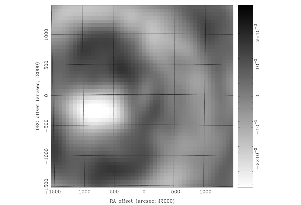
Figure 2: The Stokes Q low resolution map of 1935-692. The image is uncleaned and the high resolution CLEAN models of the sources were subtracted before imaging. The synthesized beam of the low resolution array is 5$.\mkern-4.0mu^{\prime}$5 x 3$.\mkern-4.0mu^{\prime}$9 (with a PA of $-0.2$ degrees). In a 20^′ x 10^′ box centered on the peak emission at (800$\hbox{${}^{\prime\prime}$},-250\hbox{${}^{\prime\prime}$}$), the flux is about $-15$ mJy.

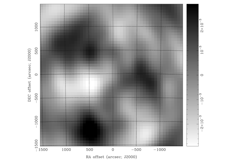
Figure 3: The Stokes U low resolution map of 1935-692. The image is uncleaned and the high resolution CLEAN models of the sources were subtracted before imaging. The synthesized beam of the low resolution array is 5$.\mkern-4.0mu^{\prime}$5 x 3$.\mkern-4.0mu^{\prime}$9 (with a PA of $-0.2$ degrees). In a 20^′ x 10^′ box centered on the peak emission at (500$\hbox{${}^{\prime\prime}$},-200\hbox{${}^{\prime\prime}$}$), the flux is about $-10$ mJy.

It is worth mentioning that we may have detected a low resolution Stokes I counterpart to the polarization signal in the field of 1935-692. We measure about 4 mJy of Stokes I flux at the location of peak emission in the low resolution Stokes U image. However, systematic errors make this a questionable detection with a SNR $\sim$ 2. As mentioned above, if this detection is real the signal is not consistent with a halo because the polarization would be well over 100$\%$. A Stokes I counterpart of GFP emission has never been seen, but 20 cm GFP is not well studied. It is possible that the emission is a new case of GFP in which the Stokes I has not been completely resolved out.

Chapter 4 Low Resolution Stokes I and the Systematic Errors

We searched for Stokes I halo signals in the low resolution data after subtracting high resolution CLEAN models of the sources. The resulting low resolution data appears to be dominated by systematic errors rather than thermal noise or a halo. Nonetheless, in the absence of a clear halo detection, upper limits can be placed on the halo flux. This requires a deeper look into the systematic errors which we now discuss. Understanding the systematic errors is also important to aid others in any future attempts at this type of work. The casual reader may skip to the next section.

One way to investigate the systematic errors is to look at data in a case where we know what to expect. For example, subtracting CLEAN models of all the sources in a field from the $uv$ data which produced the image, should yield zero (neglecting thermal errors). We refer to this treatment of the data as a “subtraction”, and to the resulting non-thermal systematic errors as the “offsets”. Our calibrator is a particularly good source for performing a subtraction because it is a bright, apparently non-varying point source in a field remarkably devoid of strong confusing emission. Unlike the subtractions used to search for halos, here we subtract data and models from the same arrays. This precludes error contributions due to differently sampled structure. Figure 5.1 shows the subtraction for the calibrator 1934-638. One night of data is shown for this object, observed the first night listed in Table 4.1 for the “6B Array”. Each point is the real part of the visibility, after subtraction, for a single antenna pair averaged over the entire night. The differences from zero are a clear indication of systematic errors. The rms of the offsets is $\sim$ 10 mJy. We do not understand this error but believe it originates with the model. The CLEAN models were made from a wide field self-calibrated image centered around 1934-638 combining all 9 nights of high resolution data listed in Table 4.1. The image has a DR of 100,000:1, and an rms of $\sim$ 150 $\mu$Jy. Unfortunately for halo searches, high DR and sensitivity in the image plane is not enough. As we see in the next section, systematic errors on the shortest baselines limit the sensitivity of the search.

Figure 1: $uv$ data with CLEAN models of the sources in the field subtracted, for 1934-638. One night of data is shown for this object taken on the first night of observations in the “6B Array” listed in Table 4.1. Each point is the real part of the visibility, after subtraction, for a single antenna pair averaged over the entire night. The offsets from zero are a clear indication of systematic errors.

1 Low Resolution Subtractions

A low resolution subtraction is the difference between low resolution data and high resolution CLEAN models of the sources. This type of subtraction can have errors in addition to the type seen on the calibrator. In particular, any large scale structure unsampled by the high resolution array will appear as differences from zero in the low resolution subtraction. Figure 5.2 shows 5 nights of low resolution subtractions on 1935-692. The visibilities for each of the 3 points are averaged over the entire night. Only the real part of the complex visibility is shown. Since we will be assuming radially symmetric models for a halo, only the real parts of the visibilities contribute. The 5 nights shown are for the data collected using phase switching in the correlator to reduce the effects of potential DC offsets. In addition, of the two correlated IF’s at 1432 MHz and 1344 MHz, only the latter is plotted. We will use these 5 nights of data to estimate upper limits to the scattered halo flux and thus upper limts on $\Omega_{\rm IGM}$. Several features are worth noting. The data points on individual baselines are consistent with thermal errors for nights 1 and 3 but are unlikely to be thermal for night 5. The rms of the offsets from zero for an individual night is about 1 mJy. Since the rms of the offsets for the calibrator in Figure 5.1 is $\sim$ 10 mJy, and the calibrator is 10 times brighter than 1935-692, the offsets are consistent with dynamic range limitations linearly proportional to the peak source in the field. Unlike the DR defined previously as the ratio of peak flux to rms in the image, we define $DR_{uv}$ here as the ratio of the peak flux to the rms, or average offset, of the $uv$ data, on a particular baseline averaged over time. This $DR_{uv}$ is most applicable to our halo search which takes place in the $uv$ plane. $DR_{uv}$ is most important for final halo analysis when evaluated on the shortest baselines. Systematic errors may result in larger scatter on the short baselines compared to the rest of the $uv$ plane. These appear in our data as offsets in the subtractions as seen in Figure 5.2. A useful determination of $DR_{uv}$ should include any contribution from the systematic offsets.

Figure 2: Five nights of low resolution subtractions on 1935-692. The visibilities for each of the 3 points are averages over the entire night. Only the real part of the complex visibility is shown, and only for the 1344 MHz IF. All nights shown are for the data collected using phase switching in the correlator to reduce the effects of potential DC offsets. It is these 5 nights of data which we use to estimate upper limits to the scattered halo flux, and thus upper limits on $\Omega_{\rm IGM}$.

Figure 3: The three plots in this figure are all visibilities for night 1 of the low resolution array after subtraction of the high resolution CLEAN models. This is the same night as the first one shown in Figure 5.2. The visibilities for each point are averages over the entire night. a) The low resolution data has been self-calibrated with the high resolution CLEAN model. Note the lack of internal consistency, within thermal errors, between data points on a given baseline. b) A low resolution subtraction on the 1432 MHz IF. c) The imaginary part of the visibility.

The rms in the residual image was our measure of progress in deciding to move on from one iteration of Imaging -$>$ Cleaning -$>$ Self-Calibrating to the next. In retrospect, we think it is crucial to monitor the offsets in the $uv$ plane, or $DR_{uv}$, as well. Although we noticed offsets in the $uv$ plane early on, we suspected they resulted from faint, uncleaned sources, and would improve as our image DR improved. Pursuing this hypothesis was nontrival and resulted in producing a wide-field image of 1935-692 with an image DR $\sim$ 77,000:1 (peak/rms), which is 7 times greater than previously obtained at the ATCA. In addition, we achieved a DR $\sim$ 100,000:1 for the calibrator source 1934-638.

Before proceeding to the upper limits, we explain which portions of the low resolution data were excluded from analysis, and why. The subtractions for the data with a $\sim$ 1 degree offset of the phase center resulted in systematic offsets several times larger than the typical rms of 1 mJy seen in Figure 5.2. This is most likely due to bandwidth smearing (even though we attempted to account for that in the data reduction). We therefore excluded those 5 nights from the halo analysis. In addition, the observations included two IF’s with a separation of 88 MHz. Figure 5.3 b) shows a typical low resolution subtraction on the 1432 MHz IF. As can be seen, the magnitude of the offsets are twice as large as those for the first night shown in Figure 5.1, which is the same plot for the 1344 MHz IF. Multi-frequency synthesis breaks down at large distances from the phase center. Since we had to CLEAN the entire field of view, we had no choice but to apply this technique to several distant sources. Looking at images of each IF separately, we have seen that cleaning resulted in more errors in the 1432 MHz data than the 1344 MHz data. We believe this to be the source of greater offsets in the low resolution subtraction and have removed the 1432 MHz data from halo analysis. We also excluded the 122 m baseline from the halo analysis. Redundancy constraints were applied to the gain calibration of the redundant spacings of the 122 meter array. However, the 122 m spacing has no redundancy and was therefore the least constrained. As a result, the 122 m baseline had an average offset of $\sim-3$ mJy. This is to be compared to the average offset of $\sim-1$ mJy obtained when only applying SELFCAL and no redundancy constraints. In any case, the 122 m spacing has little leverage in constraining the halo model.

Finally, Figure 5.3 c) shows a typical imaginary part of the low resolution subtraction. Although the offsets are larger than the real counterparts in Figure 5.2, they do not directly affect our particular halo analysis. This is because we assume a radially symmetric halo. For an isotropic central source, the only way to get a non-radially symmetric halo is with a lumpy IGM (e.g. see Katz et. al. (1996) [43]), or anisotropic illumination. A lumpy IGM could be significant. Not only would the halo produce imaginary parts to the complex visibility, but higher spatial frequencies could be created by the lumps, changing the visibility function.

Chapter 5 Upper Limits on the IGM Density

Figure 6.1 shows 5 nights of Stokes I low resolution subtracted data averaged together for each baseline (These are the 5 nights shown separately in Figure 5.2). Each square represents a data point, but the thermal error bars have been left off. To the right of each set of points, an asterisk is placed at the mean value. The larger error bars around this mean are the rms of the data points, and the smaller error bars are the error on the mean (assumed to be $\sqrt{n}$ smaller). The three sets of points are for the 31 m, 61 m, and 92 m baselines. These are the three shortest baselines in the 122 meter array which we will use to constrain the halo flux. Two Stokes I models are shown. These models use Equation 2.1 for our target source, 1935-692, with ${\mathcal{S}}_{o}$ = 1.54 Jy and Z = 3.15. The “0.05” curve is for $\Omega_{\rm IGM}$ = 0.05, and “1.00” is for $\Omega_{\rm IGM}$ = 1.00. The first feature to note in the data is that each average is negative. We think this is the result of an error in the high resolution model. Nonetheless, the error in the model is approximately constant over the three baselines (to within $\sim$ 1.5$\sigma_{mean}$). Consequently, we can not measure or constrain $\Omega_{\rm IGM}$ by measuring the absolute offset of the real part of the visibility from zero. But, as can be seen by comparison of the two models for $\Omega_{\rm IGM}$ = 0.05 and $\Omega_{\rm IGM}$ = 1.00, $\Omega_{\rm IGM}$ can also be measured or constrained by the curvature of the sampled visibility function with baseline.

Figure 1: Five nights of Stokes I low resolution subtracted data averaged together for each baseline (these are the 5 nights shown separately in Figure 5.2). Each square represents a data point, but the thermal error bars have been left off. To the right of each set of points is an asterisk at the mean. The larger error bars around this mean are the rms of the data points, and the smaller error bars are the error on the mean. The three sets of points are for the 31 m, 61 m, and 92 m baselines. These are the three shortest baselines in the 122 meter array, which we will use to constrain the halo flux. Two Stokes I models are shown. These models use Equation 2.1 for our target source, 1935-692, with ${\mathcal{S}}_{o}$ = 1.54 Jy and Z = 3.15. The “0.05” curve is for $\Omega_{\rm IGM}$ = 0.05, and “1.00” is for $\Omega_{\rm IGM}$ = 1.00.

1 ${\chi}^{2}$ Fit with Two Degrees of Freedom

Our first method to place an upper limit on $\Omega_{\rm IGM}$ is a ${\chi}^{2}$ fit with two degrees of freedom. We use Equation 2.1 for the model of a halo around 1935-692 (with ${\mathcal{S}}_{o}$ = 1.54 Jy, Z = 3.15, $\Omega_{o}=1.0$, and $H_{o}=75$). The first degree of freedom is $\Omega_{\rm IGM}$. The second degree of freedom is a parameter called “shift”, which allows a global offset for all three baselines. This is only rigorously appropriate if some systematic is affecting these three baselines similarly, which is uncertain. In this manner, $\Omega_{\rm IGM}$ is constrained only by the curvature of the measured visibility function with baseline. Figure 6.2 shows the ${\chi}^{2}$ contours. The best fit for the shift is $-0.35$. The best fit for $\Omega_{\rm IGM}$ is $-0.25$. Note that this negative value is not due to the negative offsets, because those are accounted for by the shift. Instead, the negative $\Omega_{\rm IGM}$ is due to the mean values having a rise between the 31 m and 61 m baseline in the data, as opposed to the fall predicted by the model. Taken literally, the ${\chi}^{2}$ contours indicate a 95$\%$ (or 2$\sigma$) upper limit of $\Omega_{\rm IGM}$ $<$ 0.15, but we propose a more conservative approach to the upper limit. Suppose the systematic errors on each baseline had been positive instead of negative. The magnitude of the systematic errors would be the same, but the result would be a falling visibility between the 31 m and 61 m baselines. For this reflection of the data around zero, the best fit $\Omega_{\rm IGM}$ would be 0.25, and the 95$\%$ (or 2$\sigma$) upper limit would be $\Omega_{\rm IGM}$ $<$ 0.65. (The ${\chi}^{2}$ contours for this case are just the contours in Figure 6.2 reflected about the $\Omega_{\rm IGM}$ origin.) Therefore, our 2$\sigma$ upper limit for the ${\chi}^{2}$ fit with a shift is $\Omega_{\rm IGM}$ $<$ 0.65. This result assumes an emission age for 1935-692 of $5$x$10^{7}$ yr, yet is also valid for ages between $10^{7}$ yr and $10^{8}$ yr as discussed in section 3.7.

Figure 2: (This figure has been removed to reduce size. It can be obtained by contacting Robert Antonucci at ski@ginger.physics.ucsb.edu): ${\chi}^{2}$ contours of the fit with Equation 2.1 for the model halo visibilities. A conservative approach to the upper limit reflects the data around zero and results in $\Omega_{\rm IGM}$ = 0.25, and the 95$\%$ (or 2$\sigma$) upper limit would be $\Omega_{\rm IGM}$ $<$ 0.65. The ${\chi}^{2}$ contours for this case are just the contours in the figure reflected about the $\Omega_{\rm IGM}$ origin. The contours plotted are for the probabilities of rejecting the model. Starting from the inner contour, the probabilities are: 70$\%$, 80$\%$, 90$\%$, 95$\%$, and 99$\%$.

2 ${\chi}^{2}$ Fit with One Degree of Freedom and Added Noise

There is another way to account for the systematic errors without including a global offset (or shift) as a degree of freedom. Looking at Figure 6.1, an eyeball estimate of the systematic offsets is $\sim$ 1 mJy. Assuming that the true error bars would reflect this offset, we add in quadrature, 1 mJy to the existing errors on the means. As a result, each mean with its expanded error bar is consistent with zero, and the significance of the rise from 31 m to 61 m is diminished. Figure 6.3 shows the ${\chi}^{2}$ probabilities vs. $\Omega_{\rm IGM}$ for the model fit with 1 mJy errors added in quadrature. The model and assumptions are the same as the previous ${\chi}^{2}$ test with the exclusion of the shift parameter. As expected, the best fit $\Omega_{\rm IGM}$ is still negative, but the 2$\sigma$ upper limit is $\Omega_{\rm IGM}$ $<$ 0.50.

The two ${\chi}^{2}$ tests discussed in this chapter both assume a gaussian distribution for the rms of the data points at each baseline. Since there is no a priori reason to assume gaussian errors, a non-parametric test based on the binomial distribution was performed. The results are similar to the upper limits obtained with the ${\chi}^{2}$ fits.

Figure 3: The ${\chi}^{2}$ probabilities vs. $\Omega_{\rm IGM}$ for the model fit with 1 mJy errors added in quadrature. The best fit $\Omega_{\rm IGM}$ is still negative, but the 2$\sigma$ upper limit is $\Omega_{\rm IGM}$ $<$ 0.5. The points plotted are for the probabilities of rejecting the model. Starting from the left-most pair of points, the probabilities are: 10$\%$, 20$\%$, 50$\%$, 70$\%$, 80$\%$, 90$\%$, 95$\%$, and 99$\%$.

Chapter 6 Summary

1 The IGM and Scattered Halos

Standard big bang nucleosynthesis calculations combined with observations of the primordial elements D, ³He, ⁴He, and ⁷Li predict an $\Omega_{b}~{}\sim~{}3\%$ for $H_{o}=75$. Only $\sim~{}10\%$ of these baryons are seen in stars and hot gas in clusters. To test the hypothesis that the baryons are in a diffuse ionized IGM, we searched for Thomson-scattered halos around strong high redshift radio sources.

Sholomitskii (1990) details properties of “Cosmological Halos” due to Thomson scattering of radio waves in the ionized IGM. The halos are about a degree in size and have an optical depth $\tau\sim 0.001$ for $\Omega_{\rm IGM}=0.05$, $\Omega_{o}=1.0$, $H_{o}=75$, Z = 3.5, and an assumed emission age of $5x10^{7}$ yr. Therefore a 1 Jy source would have about a 1 mJy halo, although only 5-10$\%$ of the scattered flux would be detected at 20 cm for $\sim$ 30 m baselines of an interferometer. The halos are also $\sim$ 1/3 tangentially polarized as seen in the model for the halo visibility in Equation 2.1.

To maximize scattered flux, target sources for a halo search should have strong isotropic emission and high redshift. GPS sources probably have more isotropic emission than larger double sources at high redshift. But there is no universally accepted model for these sources, and they should be used with caution. It is possible that they are too young to produce a measurable halo. Our current search is around the GPS source 1935-692 which has a 20 cm flux of 1.54 Jy, and Z = 3.15.

In general, target sources should be at $|dec|$ $\mathrel{\raise 1.29167pt\hbox{$>$\kern-7.5pt\lower 4.30554pt\hbox{$\sim$}}}$ $20^{\circ}$ if observed with an East-West array. This is to provide adequate North-South resolution for imaging confusing sources in the field. For polarized halo searches the sources should be $\mathrel{\raise 1.29167pt\hbox{$>$\kern-7.5pt\lower 4.30554pt\hbox{$\sim$}}}$ $30^{\circ}$ away from the Galactic plane. Galactic Foreground Polarization (GFP) is strongest near the plane and can completely confuse the polarization images. Before lengthly observations are made, preliminary low resolution images of candidate fields are necessary to check against GFP.

The strategy to detect halos requires low resolution baselines to sample the halo, and high resolution baselines to image the confusing sources. At 20 cm, $\sim$ 30 m spacings can sample 20 arcmin structure of the halo, while spacings out to $\sim$ 6 km can make high ($\sim$ 5 arcsec) resolution images of confusing sources. Models of confusing sources can be made using CLEAN algorithms and subtracted from the low resolution $uv$ data. Ideally, this “subtraction” results in low resolution data containing only the response of a faint halo. However, large scale confusing emission and systematic errors limit the sensitivity of the search.

2 Observations and Results

We observed 1935-692 at the ATCA for 9 nights in high resolution arrays and 10 nights in a low resolution array (see Table 4.1). We also interleaved a secondary calibrator, 1934-638, with a duty cycle chosen to result in a dynamic range (DR) comparable to that of the target source. We found the calibrator observation to be invaluable for investigating systematic errors, and highly recommend its inclusion in any observing program. Redundancy of the shortest spacings in the low resolution array was used to help calibrate antenna gains.

High resolution images with high DR were made for 1935-692 and 1934-638. These were used to make CLEAN models of sources for both calibration of, and subtraction from, the low resolution data. We achieved DR’s (peak/rms) of 77,000:1 and 100,000:1, for 1935-692 and 1934-638 respectively. These are significant increases over the previously obtained DR’s at the ATCA of around 10,000:1.

Low resolution polarization imaging of 1935-692 revealed large scale polarized emission in both Stokes Q and U. The emission is not centered around 1935-692 and is more consistent with GFP than with a cosmological halo. GFP is characterized by having little or no detectable Stokes I emission, resulting in apparent polarization fractions $>>$ 100$\%$. Halo models unequivocally predict detected polarization fractions $<100\%$. Internal consistency and checks with the calibrator lead us to believe the the emission is real. While it is not absolutely certain that the signal is truly GFP, the emission prevents us from placing meaningful limits on polarized scattered halo flux.

The Stokes I analysis for halos was limited by systematic errors. We obtained high DR in the image plane. However, it is the $DR_{uv}$ in the $uv$ plane on the shortest baselines averaged over time which is most important. The $DR_{uv}$ is the ratio of the peak flux to the rms, or average offset, on a particular baseline averaged over some time interval. For 1935-692, we had an rms $\sim$ 1 mJy for the offsets on an individual night. With a peak flux of ${\mathcal{S}}_{o}$ = 1.54 Jy, this is a $DR_{uv}\sim$ 1,500:1 on the shortest baselines in the 122 meter array. Hindsight has shown that monitoring the $DR_{uv}$ as a measure of progress is more meaningful than the image plane DR since the halo analysis takes place in the $uv$ plane. We recommend monitoring $DR_{uv}$ on both target and calibrator source, and on high and low resolution subtractions (if multiple arrays are used).

We think our systematic errors derive ultimately from imperfections in the CLEAN models of the sources, but do not understand the origin. The systematic errors affected different segments of our data differently, and we excluded from the halo analysis those segments with largest errors. One excluded segment is 5 nights of data taken with a $\sim$ 1 degree phase offset from the pointing center. The other segment excluded is one of the two IF’s for which the multi-frequency synthesis produced a poorer model.

Figure 6.1 shows the low resolution subtracted data used for halo analysis. Each baseline has a negative offset which we think is due to a systematic error, as opposed to a difference indicative of real emission on the sky. The systematics prevent any clear detection or tight limit on a halo. Nonetheless, an upper limit can be placed on any scattered halo flux and thus on $\Omega_{\rm IGM}$. Our first method to determine an upper limit is a ${\chi}^{2}$ fit to Equation 2.1 with 2 degrees of freedom. In this fit, one free parameter is $\Omega_{\rm IGM}$. The other free parameter is a constant “shift”, included to account for the systematic, negative offset of the data. This allows a fit of $\Omega_{\rm IGM}$ through the relative changes of the baselines. Our upper limit based on this method is $\Omega_{\rm IGM}<0.65~{}(2\sigma,95\%)$.

There is another way to account for the systematic errors without assuming a global offset (or shift). We can accomodate the offset by adding 1 mJy in quadrature to the existing errors on the means for each baseline. As a result, each mean with its expanded error bar is consistent with zero, and the significance of the rise (probably unphysical) from 31 m to 61 m is diminished. With this ${\chi}^{2}$ fit the 2$\sigma$ upper limit is $\Omega_{\rm IGM}$ $<$ 0.50.

Chapter 7 Conclusion

We would like the reader to see that the search for halos has motivations in fundamental cosmology and that this current attempt finds $\Omega_{\rm IGM}<1$. In addition, this thesis is meant to provide helpful hints for others wishing to search for cosmological halos at the ATCA, WSRT, or the VLA.

Although the halo project is very difficult, it is robust against false detections. An observer can have confidence in a detection if 1) The radial profile follows Equation 2.1; 2) There is a corresponding low signal on the imaginary part of the visibilities; 3) The predicted magnitude and direction of polarization is seen; and 4) A low redshift calibrator produces no halo since the density of ionized gas at low Z greatly decreases the optical depth. In addition, the ${\mathcal{S}}_{o}$ and Z dependence in Equation 2.1 can be used to confirm $\Omega_{\rm IGM}$ in a survey of different objects. Furthermore, Equation 2.1 can be used to coadd multiple halo visibilities of the same, or different, sources observed on any telescope arrays. Our experience has been that both systematic errors in Stokes I and large size-scale polarized confusion can prevent reaching thermal sensitivity on the short baselines where it is needed. Therefore, we suggest that future observing programs involve several halo targets, and accepting sources with only modest thermal SNR estimates. Coadding the results of the survey makes full use of all healthy data, minimizes superfluous integration time, and hopefully averages down systematic errors. Finally, with the increased sensitivity becoming available because of receiver improvements, it becomes affordable to target extended doubles rather than GPS sources. Though fainter, the extended sources should be safer regarding assumptions about isotropic emission and ages $\mathrel{\raise 1.29167pt\hbox{$>$\kern-7.5pt\lower 4.30554pt\hbox{$\sim$}}}10^{7}$ years.

References

- [1] Walker, T., Steigman, G., Schramm, D., Olive, K., and Kang, H. Astrophysical Journal 376, 51 (1991).
- [2] Izotov, Y., Thuan, X., and Lipovetsky, V. Astrophysical Journal 435, 647 (1994).
- [3] Songaila, A. et al. Nature 368, 137 (1994).
- [4] Wampler, E. et al. Astronomy and Astrophysics 316, 33 (1996).
- [5] Webb, J. et al. Nature 388, 250 (1997).
- [6] Tytler, D., Fan, X., and Burles, S. Nature 381, 207 (1996).
- [7] Burles, S. and Tytler, D. Submitted to Science. (1996).
- [8] Hogan, C. astro-ph/9712031 .
- [9] Yang, J. et al. Astrophysical Journal 186, 493 (1984).
- [10] Spite, F. and Spite, M. Astronomy and Astrophysics 115, 56 (1984).
- [11] Thorburn, J. Astrophysical Journal 421, 318 (1994).
- [12] Copi, C., Schramm, D., and Turner, M. Science 267, 192 (1995).
- [13] Persic, M. and Salucci, P. Monthly Notices of the Royal Astronomical Society 258, 14 (1992).
- [14] Kurki-Suonio, H. et al. Astrophysical Journal 353, 406 (1990).
- [15] Alcock et al. Astrophysical Journal 486, 697A (1997).
- [16] Gunn, J. and Peterson, B. The Astrophysical Journal 142, 1633 (1965).
- [17] Steidel, C. and Sargent, W. Astrophysical Journal 318, L11 (1987).
- [18] Webb, J. Monthly Notices of the Royal Astronomical Society 255, 319 (1992).
- [19] Giallongo, E., Cristiani, S., and Trevese, D. Astrophysical Journal 398, L9 (1992).
- [20] Davidson, A., Kriss, G., and Zheng, W. Nature 380, 47 (1996).
- [21] Hogan, C., Anderson, S., and Rugers, M. Astronomical Journal 113, 1495 (1997).
- [22] Jakobsen, P. et al. Nature 370, 35 (1995).
- [23] Reimers, D. et al. astro-ph/9707173 .
- [24] Sholomitskii, G. B. and Yaskovitch, A. L. Soviet Astronomy Letters 16, 383 (1990).
- [25] Sholomitskii, G. B. Soviet Astronomy 35, 15 (1991).
- [26] Sholomitskii, G. B. Soviet Astronomy 36, 222 (1992).
- [27] O’Dea, C. P. Submitted to PASP. (1997).
- [28] Haslam, G. et al. Astronomy and Astrophysics 47 (1982).
- [29] Antonucci, R. and Ulvestad, J. Astrophysical Journal 294, 158A (1985).
- [30] Vallee, J. Astronomy and Astrophysics 239, 57 (1990).
- [31] Andreani, P. et al. Astrophysical Journal 459, L49 (1996).
- [32] Begelman, M., Blandford, R., and Rees, M. Rev. Mod. Phys. 56, 255 (1984).
- [33] Scheuer, P. Monthly Notices of the Royal Astronomical Society 277, 331 (1995).
- [34] Wieringa, M. et al. Astronomy and Astrophysics 268 (1993).
- [35] Sault, R., Teuben, P., and Wright, M. ASP Conference Series 77, 433 (1995).
- [36] Sault, R., Killeen, N., and Kesteven, M. ATNF Technical Memo No. 39.3015 (1991).
- [37] Conway, J., Cornwell, T., and Wilkinson, P. Monthly Notices of the Royal Astronomical Society 246, 490 (1990).
- [38] Sault, R. and Wieringa, M. Astronomy and Astrophysics Supplement Series 108, 589 (1994).
- [39] Högbom, J. Astronomy and Astrophysics Supplement Series 15, 417 (1974).
- [40] Pearson, T. and Readhead, A. Astronomy and Astrophysics 22, 97 (1984).
- [41] Noordam, J. and de Bruyn, A. Nature 84, 597 (1982).
- [42] Wieringa, M. Experimental Astronomy 2, 203 (1992).
- [43] Katz, N. et al. Astrophysical Journal 457, L57 (1996).