A Photometric and Weak Lensing Analysis of the $z=0.42$ Supercluster MS0302+17

Abstract

We perform a weak lensing and photometric study of the $z=0.42$ supercluster MS0302+17 using deep $I$ and $V$ band images taken with the UH8K CCD mosaic camera at the CFHT. We use archival ROSAT HRI data to estimate fluxes, gas masses and, in one case, the binding mass of the three major clusters. We then use our CCD data to determine the optical richness and luminosities of the clusters and to map out the spatial distribution of the early type galaxies in the supercluster and in other foreground and background structures. We measure the gravitational shear from a sample of $\simeq 30,000$ faint background galaxies in the range $22\lesssim m_{I}\lesssim 26$ and find this correlates strongly with that predicted from the early type galaxies if they trace the mass with $M/L_{B}\simeq 250h$. We make 2-dimensional reconstructions of the mass surface density. These recover all of the major concentrations of galaxies and indicate that most of the supercluster mass, like the early type galaxies, is concentrated in the three X-ray clusters, and we obtain mean mass-to-light ratios for the clusters of $M/L_{B}\simeq 260h$. Cross-correlation of the measured mass surface density with that predicted from the early type galaxy distribution shows a strong peak at zero lag (significant at the $\simeq 9$-sigma level), and that at separations $\gtrsim 200h^{-1}$kpc the early galaxies trace the mass very accurately. This conclusion is supported by cross-correlation in Fourier space; we see little evidence for any variation of $M/L$ or ‘bias’ with scale, and from the longest wavelength modes with $\lambda=1.5-6h^{-1}$Mpc we find $M/L\simeq(280\pm 40)h$, quite similar to that obtained for the cluster centers. We discuss the implication of these results for the cosmological density parameter.

1 Introduction

Weak lensing, in the sense of the statistical distortion of the shapes of faint background galaxies, has now been measured for quite a number of clusters: Tyson et al. (1990); Bonnet et al. (1993); Fahlman et al. (1994); Bonnet et al. (1994); Dahle et al. (1994); Mellier et al. (1994); Fort & Mellier (1994); Smail & Dickinson (1995); Tyson & Fischer (1995); Fort et al. (1996); Seitz et al. (1996); Bower & Smail (1997); Smail et al. (1997); Fischer et al. (1997); Fischer & Tyson (1997), and provides a powerful and direct measurement of the total mass distribution in clusters. Following the pioneering attempt of ?) using photographic plates, several groups (Brainerd et al. (1996); Dell’Antonio & Tyson (1996); Griffiths et al. (1996); Hudson et al. (1998)) have reported measurements of the ‘galaxy-galaxy lensing’ effect due to dark halos around galaxies, and there have also been attempts to estimate the shear due to large-scale structure (Valdes et al. (1983), Mould et al. (1994), Schneider et al. (1998)). Most of these studies have been made with fairly small CCD detectors; this severely limits the distance out to which one can probe the cluster mass distribution and also limits the precision of galaxy-galaxy lensing and large-scale shear studies.

Here we present a weak lensing analysis of deep $I$ and $V$ photometry of the field containing the $z\simeq 0.42$ supercluster MS0302+17 taken with a large 8192$\times$8192 pixel CCD mosaic camera (the UH8K; Luppino et al. (1995)) mounted behind the prime focus wide field corrector on the CFHT. The field of view of this camera on this telescope measures $0^{\circ}.5$ on a side, and greatly increases the range of accessible scales, and should yield improved precision for large-scale and galaxy-galaxy shear measurements. Our goal here is to explore the total (dark plus luminous) mass distribution in this supercluster field and see how this relates to the distribution of super-cluster galaxies and the X-ray emitting gas.

The target field, centered roughly on $\rm{RA}=3^{h}5^{m}24^{s}.0,\rm{DEC}=17^{\circ}18^{\prime}0^{\prime\prime}.0$, (J2000) contains three prominent clusters in a supercluster at $z\simeq 0.42$. The first of these clusters to be found, CL0303+1706, was detected optically by ?). It has a redshift of $z=0.418$, a velocity dispersion $\sigma_{v}=912$ km/s, and was the the target of an Einstein IPC pointed observation. This observation revealed two sources within $\sim 1^{\prime}$ of the position given by Dressler and Gunn, one of which, it is now apparent, coincides with densest and most massive concentration of galaxies in the cluster, and which has an X-ray luminosity $L_{\rm X}\simeq 3.0h_{50}^{-2}\times 10^{44}$ erg/s. Analysis of the IPC image and optical follow up by the EMSS team Gioia et al. (1990); Stocke et al. (1991); Gioia & Luppino (1994) revealed the presence of the two neighboring clusters MS0302+1659 and MS0302+1717 with redshifts $z=0.426,0.425$ and X-ray luminosities $L_{\rm X}\simeq 5.0\times 10^{44}h_{50}^{-2}$erg/s $4.3\times 10^{44}h_{50}^{-2}$ erg/s. The fluxes here are taken from the analysis of the IPC images by ?), who also obtained redshifts for a large number of galaxies in the the two X-ray brighter clusters, and obtained velocity dispersions of and 921 and 821 km/s respectively. ?) have reported a velocity dispersion of 646 km/s for MS0302+1659 based on 27 redshifts and ?) have presented an extended catalog of redshifts for this cluster. Deep optical CCD images of MS0302+1659 were taken by ?) which revealed the presence of a pair of giant arcs and additional photometry was taken by ?) who found evidence for variability of features in one of the arcs.

The angular separations of the clusters CL0303+1706, MS0302+1659 and MS0302+1717 (which we will refer to as CL-E, CL-S, CL-N respectively) are $\theta_{\rm NE}=17^{\prime}.64$, $\theta_{\rm NS}=18^{\prime}.49$, and $\theta_{\rm SE}=14^{\prime}.04$. Assuming an Einstein de Sitter universe, the angular diameter distance is $D=2cH_{0}^{-1}(1-(1+z)^{-1/2})/(1+z)$ so $D(z=0.42)\simeq 679h^{-1}$Mpc and the physical scale is 3.29$h^{-1}$ kpc/arcsec or 197$h^{-1}$ kpc/arcmin. For pure Hubble flow the line of sight physical separation is $\Delta r^{\parallel}=(1+z)^{-5/2}c\Delta z/H_{0}$ or about $1.24\Delta zh^{-1}$Gpc. Fabricant et al. found $\Delta z_{\rm NS}=0.0009\pm 0.0012$ from which we infer that the separation of the EMSS clusters in redshift space is $\Delta r_{\rm NS}\simeq 3.8h^{-1}{\rm Mpc}$, and is primarily transverse to the line of sight ($\Delta r^{\parallel}_{\rm NS}\simeq 1.1\pm 1.5h^{-1}{\rm Mpc}$, $\Delta r^{\perp}_{\rm NS}\simeq 3.6h^{-1}{\rm Mpc}$). The Dressler-Gunn cluster E lies about $\Delta r^{\parallel}_{\rm NE}\simeq 9h^{-1}{\rm Mpc}$ in front of the two EMSS clusters. The parallel distance components may be somewhat distorted by peculiar motions. For an empty open cosmology $D=0.5cH_{0}^{-1}(1-(1+z)^{-2})$ so $D(z=0.42)\simeq 756h^{-1}$Mpc and $\Delta r^{\parallel}=(1+z)^{-2}\Delta zc/H_{0}$ or about $1.49\Delta zh^{-1}$Gpc, in which case the transverse and line of sight physical dimensions are larger than the EdS values by about $11$% and $20$% respectively. For an extreme $\Lambda$ dominated model with $\Omega_{\Lambda}=1$, $\Omega_{m}=0$, $D=czH_{0}^{-1}/(1+z)$ and so $D(z=0.42)\simeq 887h^{-1}$Mpc and $\Delta r^{\parallel}=(1+z)^{-1}\Delta zc/H_{0}$ or about $2.11\Delta zh^{-1}$Gpc, in which case the transverse and line of sight physical dimensions are larger than the EdS values by about $30$% and $69$% respectively. The parallel distance components may be somewhat distorted by peculiar motions.

This field was chosen for weak lensing as the high velocity dispersions and high X-ray luminosities of these clusters (along with the presence of arcs in one case) lead one to suspect that they might be potent lenses. Also, the whole system fits conveniently within the approximately $30^{\prime}\times 30^{\prime}$ field of view of the UH8K camera. This system provides an example of a quasi-linear system in the process of formation and it is of interest to see if weak lensing can detect, or constrain, the presence of ‘bridges’ of dark matter that can be expected between clusters Bond et al. (1996). However, our main goal is to explore the correlation between mass and optical luminosity density to obtain estimates of the mass to luminosity ratio $M/L$, or equivalently the inverse of the ‘bias factor’, (using the methodology of ?), ?)) and to see if this varies with scale. A source of systematic uncertainty in weak lensing mass estimates is the still largely unknown redshift distribution of the faint background galaxies. As a check we compare our mass estimates for the centers of the clusters with mass estimates from the velocity dispersions and, in one case, an estimate of the X-ray gas temperature.

The outline of the paper is as follows: In §2 we review the existing X-ray and optical spectroscopy results. We obtain improved fluxes and positions from archival ROSAT HRI observations. We make crude estimates of the central gas masses and, for CL-S estimate the central total mass from an ASCA temperature obtained by ?) and compare with the optical velocity dispersion. In §3 we explore the optical structure of the supercluster. We briefly describe the image processing; present a color image of the field; and show the size-magnitude distribution for the $\sim 44,000$ objects detectable at $>6$-sigma significance. We describe the somewhat non-standard photometric system we are using, and compute expected colors as a function of redshift and galaxy type. We plot the position, color and luminosities of the brighter galaxies, and we compute counts of galaxies as a function of magnitudes for regions around the clusters and for the complementary field region. In the absence of extensive redshift information it is hard to accurately measure the total optical luminosity distribution due to the confusing effect of foreground structures. If we restrict attention to the narrow band of $V-I$ color occupied by the early type galaxies at the supercluster redshift this foreground clutter is effectively removed and we obtain a cleaner picture of the distribution of these galaxies and obtain estimates of the optical richness and luminosity functions for the three X-ray bright clusters.

In §4 we present the weak lensing analysis. In §4.1 we describe how we select the faint galaxies used to measure the shear and how we calibrate the relation between the observed image polarization and the gravitational shear. The calibration and also the correction for point spread function anisotropy is described more fully elsewhere Kaiser (1998). Our shear analysis features an optimized weighting scheme, and we show how the weight is distributed in magnitude and on the size-magnitude plane. In §4.2 we predict the dimensionless surface density $\kappa(\theta)=\Sigma_{m}/\Sigma_{\rm crit}$ assuming that early type galaxy light traces the mass with some a constant $M/L$. We do this both for a narrow slice around the supercluster redshift and also for a broader range of $V-I$ color, corresponding to a range of redshifts $0.2\lesssim z\lesssim 0.6$, and which includes a significant contribution from a foreground structure at $z\simeq 0.3$. In §4.3 we correlate the measured shear with that predicted from the early type galaxy distribution. In §4.4 we perform 2-dimensional mass reconstructions and compare these with the constant $M/L$ prediction. In §4.5 we estimate central mass-to-light ratios for the three X-ray bright clusters, and we compare these with velocity dispersions and X-ray temperature information. In §4.6 we compute the real space light-mass cross-correlation function to obtain a more precise estimate of the $M/L$ parameter and we compare the profile of the mass-light cross-correlation function and that of the luminosity auto-correlation function. We also perform the cross-correlation in Fourier space in order to see if there is any evidence for ‘scale dependent biasing’ (i.e. variation of the $M/L$ parameter with scale).

2 X-Ray Properties

In this section we review the published X-ray results and obtain improved fluxes and positions from archival ROSAT HRI observations. We make crude estimates of the central gas masses and, for CL-S estimate the central total mass from an ASCA temperature obtained by Henry and compare with the optical velocity dispersion.

The Einstein IPC image from the Einstein database is shown in the left hand panel of figure 1, with the circles indicating the locations of the clusters. Only the region where we have optical photometry coverage is shown. Analysis of these data by ?) gave estimates of the luminosities for these clusters quoted in the Introduction. The identification of the target cluster was originally somewhat confused as the cluster is quite extended, and the location provided by Dressler and Gunn was displaced somewhat to the West from what is now seen to be the cluster center, and lay right between the two sources on the left with $\delta\simeq 17^{\circ}19^{\prime}$. There is some indication of extended emission around CL-N, but the situation is somewhat confused by the shadowing of the support structure.

There have been two further observations of the field with the ROSAT HRI which are now in the public domain. One of these was of $\sim 3.5\times 10^{4}$s integration time and was centered on CL-S, but also contains CL-E, while the other of $\sim 9\times 10^{4}$s integration contains all three clusters. These have higher resolution and higher astrometric precision than the IPC data. To analyze these data we used Steve Snowden’s software Snowden (1998) to generate a model for the particle background for each pointing, which we subtract, and also to generate a detailed exposure map which we divide into the subtracted image to correct for vignetting. We then mask out objects detected at $>4$-sigma significance level and take the mean of what is left to obtain an estimate of the sky background, which we also subtract. The neutral hydrogen column density along the line of sight is $N_{H}=1\times 10^{21}$cm^-2 Dickey & Lockman (1990) from which we find (assuming a Raymond-Smith spectrum with observed temperature of $3.43$keV and $0.25$ times solar metallicity) that one HRI count per second corresponds to an unabsorbed bolometric flux of $1.06\times 10^{-10}$ erg/sec/cm² (for the often quoted passbands of $0.2-4.5$keV and $0.5-2.0$keV the corresponding conversion factors are $7.75\times 10^{-11}$ erg/sec/cm² and $3.79\times 10^{-11}$ erg/sec/cm²). A smoothed surface brightness image is shown in figure 2. The unsmoothed HRI image shows that most of the other sources are still unresolved (and are therefore most probably not emission from cluster gas). The smoothed HRI image also shows the extended emission around CL-N, though now without the masking effect of the IPC ribs. CL-E is seen to be extended towards the NW, and at higher resolution appears to have a second core. This bimodality is also seem in the highly non-circular distribution of cluster galaxies so it would appear that this is most probably a merger event. The azimuthally averaged surface brightness profiles for CL-N, CL-S are shown in figure 2. CL-N appears to have a slope with index $\gamma\sim-1$ (where $I(\theta)\propto\theta^{\gamma}$) with significant emission extending to $\theta\sim 100-200^{\prime\prime}$. CL-S has a slightly steeper slope $\gamma\sim-1.4$ within $\theta\simeq 50^{\prime\prime}$, outside of which radius the emission drops sharply and there is no statistically significant flux detectable at larger radii. This cluster is remarkably compact as compared to more typical bright X-ray clusters which have cores with essentially flat emission profiles extending to about this radius and with most of the gas residing at larger radii.

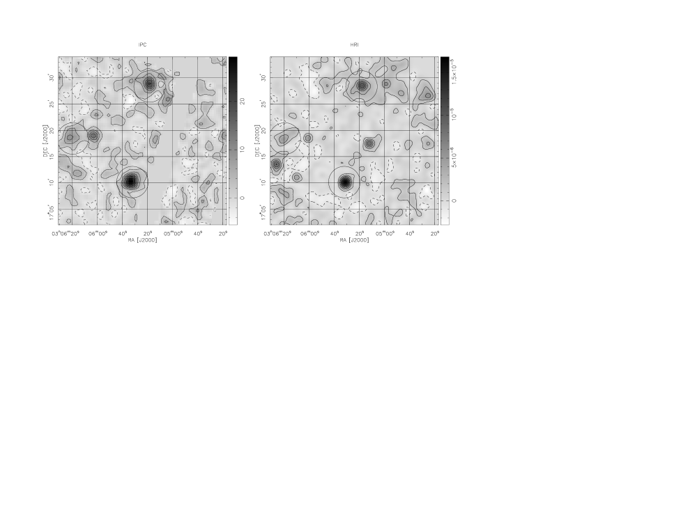
Figure 1: left hand panel shows the IPC X-ray image from the Einstein archive. The units of intensity are in IPC counts per second per square arcmin. The circles show the optical cluster centroids. Right hand panel shows a composite of the two HRI pointings, smoothed with a $35^{\prime\prime}$ Gaussian. The intensity units are HRI counts per second per $(5^{\prime\prime})^{2}$ pixel.

Figure 2: Upper panel shows the azimuthally averaged surface brightness profiles for the clusters CL-S (squares) and CL-N (circles). CL-E is not shown as it is clearly non-circular. Lower panel shows the gas density profile obtained by direct deprojection as described in the text.

Assuming spherical symmetry, the rest-frame surface brightness at impact parameter $r$ is

$$I_{\rm rest}(r)={1\over 4\pi}\int dz\;\epsilon_{\rm ff}(\sqrt{r^{2}+z^{2}})$$ (1)

where the Bremsstrahlung emissivity is $\epsilon_{\rm ff}=\alpha_{\rm ff}n_{p}^{2}T^{1/2}$ where $\alpha_{\rm ff}\simeq 3\times 10^{-27}$erg cm³ s^-1 K^-1/2 Sarazin (1988). Approximating the integral as a sum over cubical ‘voxels’, the observed surface brightness for a pixel at radius $i$ pixels from the cluster center in an image with pixel size $\Delta\theta$ is

$$I_{\rm obs}(i)={a_{0}\omega_{l}\Delta\theta\over 4\pi(1+z)^{5}}\sum\limits_{j}F(\sqrt{i^{2}+j^{2}})$$ (2)

with $F(i)\equiv\epsilon_{\rm ff}(a_{l}\omega_{l}i\Delta\theta)$. We can invert the projection sum numerically to obtain $F(i)=4\pi(1+z)^{5}(a_{0}\omega_{l}\Delta\theta)^{-1}\tilde{I}(i)$ where $I(i)\equiv\sum\tilde{I}(\sqrt{i^{2}+j^{2}})$, and hence the gas density:

$$n_{p}(r)=\left({4\pi(1+z)^{5}\tilde{I}(r/a_{l}\omega_{l}\Delta\theta)\over a_{0}\omega_{l}\Delta\theta T^{1/2}\alpha_{\rm ff}}\right)^{1/2}$$ (3)

The gas density profiles are shown in the lower panel of figure 2 from which we estimate gas masses within radius corresponding to $1^{\prime}.5$ of $M_{S}\simeq 2.5\times 10^{12}h^{-5/2}M_{\odot}$, $M_{N}\simeq 2.8\times 10^{12}h^{-5/2}M_{\odot}$.

?) has obtained an ASCA spectrum for CL-S from which he finds a rest-frame temperature of $4.6\pm 0.8$keV. Assuming isothermality, the total mass interior to $r$ is $M(r)=-(kTr/G\mu m_{p})d\ln n/d\ln r$, and using a logarithmic slope of $d\ln n/d\ln r=-1.5$ and a mean molecular weight $\mu=0.6$ we find $M(<r=167h^{-1}{\rm kpc})=4.25\times 10^{13}h^{-1}M_{\odot}$, this radius corresponding to the angular scale of $50^{\prime\prime}$. Combining these results, we find a gas fraction for CL-S of $M_{\rm gas}/M_{\rm tot}\simeq 0.06h^{-3/2}$. Both the gas and total mass estimates should be considered to be lower bounds, as there may be emission at larger radii which we cannot detect and one could also imagine that the cluster has an extended dark matter halo which these central X-ray observations cannot constrain. It is interesting to compare $(kT/G\mu m_{p})^{1/2}\simeq 854$km/s with the observed velocity dispersion of $921$km/s. As we shall see, the galaxies in the cluster are, like the observable gas, highly concentrated and have a very similar scale length, so it is reassuring that the kinetic energy per unit mass is essentially the same for the gas and for the galaxies. The high temperature and very small size of the cluster indicate a very short sound crossing time $t=r/c_{s}\simeq 2\times 10^{8}$yr.

The inferred gas density in the very center of CL-S (at around $15^{\prime\prime}$ or about $50h^{-1}$kpc say) is $n\simeq 1.4\times 10^{-2}h^{-1/2}{\rm cm}^{-3}$, implying a cooling rate of about $\Gamma\sim 1.4\times 10^{-18}h^{-1/2}{\rm s}^{-1}$ or a cooling time $t_{\rm cool}\sim 2.2\times 10^{9}h^{1/2}{\rm yr}$, as compared to the age of the Universe at $z=0.42$ of $t\simeq 3.9\times 10^{9}h^{-1}{\rm yr}$ for $\Omega=1$, or $t\simeq 7.1\times 10^{9}h^{-1}{\rm yr}$ for an open $\Omega\simeq 0$ cosmology, so the ratio of the cooling time to the age of the Universe $t_{\rm cool}/t(z=0.42)$ is in the range $(0.3-0.5)h^{3/2}$ so we are dealing with a strong, but still quasi-static, cooling flow. We estimate the gas loss rate as $\dot{M}\sim 100-200M_{\odot}$/yr. At a radius of $50^{\prime\prime}$ the density is an order of magnitude lower, so the cooling time is an order of magnitude larger and, for $h=0.7$, $t_{\rm cool}/t(z=0.42)$ lies in the range 1.7-3.0 so the cooling is somewhat larger than the age of the Universe. However, for low $\Omega$, and in the absence of heat sources, much of the gas we see will by now have dropped out of the cooling flow.

The HRI derived positions, count rates, fluxes luminosities of the three clusters are summarized in table 1. The agreement between our luminosities and those of ?) is generally very good. For CL-S, for instance, and for the $0.2-4.5$keV band, we find $L=4.9\pm 0.4\times h_{50}^{-2}10^{44}$erg/s whereas they find $L=5.0\pm 0.8\times h_{50}^{-2}10^{44}$ erg/s.

Cluster	RA(J2000)	DEC(J2000)	$r$ [cts/s]	$f_{\rm bol}$ [erg/s/cm2]	$h_{50}^{2}L_{\rm bol}$ [erg/s]
CL-S	$3^{h}05^{m}31^{s}.49$	$17^{\circ}10^{\prime}16^{\prime\prime}.32$	$7.1\pm 0.5\times 10^{-3}$	$7.6\pm 0.6^{-13}$	$6.8\pm 0.5\times 10^{44}$
CL-E	$3^{h}06^{m}18^{s}.98$	$17^{\circ}18^{\prime}33^{\prime\prime}.91$	$3.8\pm 0.7\times 10^{-3}$	$4.0\pm 0.8^{-13}$	$3.6\pm 0.7\times 10^{44}$
CL-N	$3^{h}05^{m}17^{s}.81$	$17^{\circ}28^{\prime}37^{\prime\prime}.64$	$5.6\pm 0.6\times 10^{-3}$	$6.0\pm 0.7^{-13}$	$5.4\pm 0.6\times 10^{44}$

Table 1: Cluster X-ray Properties. Positions are locations of peaks of the smoothed HRI image. Count rates, fluxes and luminosities are for $1^{\prime}.5$ radius apertures centered on the given position, except for CL-E where we include the flux in a second aperture centered on the secondary feature to the NW of the main cluster.

3 Optical Photometry

3.1 Data Acquisition and Processing.

In September 1995, we obtained deep images of the MS0302 supercluster using the UH8K CCD camera mounted at the prime focus of the CFHT. At an image scale of $\simeq 0^{\prime\prime}.207$/pixel, the 8192$\times$8192 pixel CCD mosaic spans a field of view of $\sim$29^′ on a side. The images were taken in superb observing conditions: photometric sky with $\sim 0^{\prime\prime}.6$ seeing. Multiple 15 minute exposures were taken, with the telescope shifted slightly ($\sim 20-30^{\prime\prime}$) between exposures, in order to facilitate flat fielding and the construction of a seamless final image. In all, 11 I-band images and 6 V-band images were used to give final exposure times of the summed images of 9900s and 5400s respectively.

The image processing was rather involved, and is described more fully elsewhere Kaiser et al. (1988) but essentially consists of four phases; pre-processing of original images; registration to obtain the transformation from chip to celestial coordinates; warping and averaging to produce the final images (and also auxiliary files describing the variation of photon counting noise, point spread function shape etc); and finally the generation of catalogs of objects.

In the pre-processing we first generated a median sky image or ‘super-flat’ for each chip and each passband and divided this into the data images. The super-flat was also used to identify bad columns, traps, and other defects, which were flagged as unreliable. To further suppress residual variations in the sky background level we then subtracted from the images a smooth local sky background estimate formed from the depths of the minima of a slightly smoothed version of the super-flat divided data images.

In the registration phase we took the locations of stars measured on the data chips, along with stars with known accurate celestial coordinates from the USNOA catalog Monet (1998) and solved in a least square manner for a set of low order polynomials — one for each of the $2{\rm K}\times 4{\rm K}$ images — which describe the mapping from rectilinear chip coordinates to celestial coordinates. We computed a sequence of progressive refinements to the transformation. The final solution gave transformations with a precision of about 5 milli-arcsec, which accurately correct for field distortion, atmospheric refraction, and the layout of the chips in the detector, and also any other distortions produced by inhomogeneities of the filters and/or mechanical distortion of the detector.

In the image mapping phase we applied the spatial transformations to generate a quilt of slightly overlapping images covering a planar projection of the celestial sphere. We chose the ‘orthographic’, shape-preserving projection Greisen & Calabretta (1995) with tangent point at $(\alpha,\delta)_{\rm J2000}=(3^{h}05^{m}24^{s}.0,17^{\circ}18^{\prime}0^{\prime\prime}.0)$ and rotation angle of $2^{\circ}.635$ (this being chosen to render the star trails aligned with the vertical axis of the final image to facilitate masking of these artifacts). Cosmic ray pixels and satellite trails etc. were identified by comparing each image section with the median of a stack of images taken in the same passband, and were flagged as unreliable. The final images were made by simple averaging of the non-flagged pixels in the stack of warped images. The combination of the mosaic chip geometry layout, the pattern of shifts for the exposures, and the presence of unreliable data of various types resulted in a somewhat non-uniform sky noise level, which we kept track of by making an auxiliary image of the sky noise. The FWHM of stars in these stacked images were approximately $0^{\prime\prime}.60$. We also generated a detailed model for how the point spread function (psf) shape varies across the final image (this is quite complicated as the psf shape changes discontinuously across chip boundaries) and we apply this below to correct the measured galaxy shapes to what they would have been if measured with a telescope with perfectly circular psf.

A color image generated from the summed V and I band exposures is shown in figure 3. The Dressler-Gunn cluster CL-E is clearly visible close to the Eastern edge of the field as an agglomeration of early-type galaxies with very similar color. The two X-ray selected clusters can be seen fairly clearly, and the giant arcs in the Southern cluster are apparent. Both of these clusters contain galaxies with the same color as in CL-E, but in both cases there are also bright bluer galaxies in the vicinity, suggesting that there is some foreground contamination.

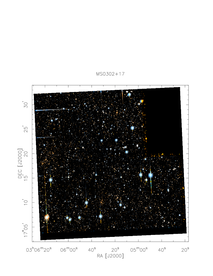
Figure 3: Color image generated from the summed V and I band images. This is a heavily reduced (de-magnified) image of the field derived from the final averaged images (which have a re-sampled pixel scale of $0^{\prime\prime}.15$ and cover $12,000^{2}$ pixels). In order to show both the faint background galaxies and the much brighter foreground galaxies, the brightness of each pixel here was taken to be proportional to the logarithm of the sum of the two V and I-band images, and the individual intensities are such that the red and blue signals are in the same proportion as in the linear I, V images (with a constant multiplicative scaling applied to the blue value) and the green signal is the mean of the red and blue signals. Thus this is not a true 3-color image (which would look much whiter), but is useful to distinguish the different galaxy types present.

After registering and summing the images we ran our ‘hierarchical peak finding algorithm’ to detect objects (Kaiser et al. (1995), Kaiser et al. (1988)) on each of the I- and V-band images and then ran our aperture photometry and shapes analysis routines to compute magnitudes, radii and other properties of the objects. For each of the $I,V$ catalogs we also estimated magnitudes using the summed image for the other passband (but with the same center and aperture radius) in order to provide accurate color information. We also constructed a combined ‘I+V’ catalog in which, if an object was detected in both V and I then we include only the most significant detection, whereas if the object was only detected in one passband then the information for that filter only is included. This is the primary catalog we use in the analysis below. To remove spurious detections from the diffraction spikes around bright stars and trails caused by poor charge transfer for saturated pixels, we generated a mask consisting of the rectangles shown in figure 11, and objects lying within these rectangles were not used in the following analysis. The combined catalog contains about 44,000 objects detected at $>6$-sigma significance. The total unmasked area is $A=0.165$ square degrees, so the number density of these objects is about 74 per square arcmin. The size-magnitude distribution for the combined catalog is shown in figure 4, from which it can be seen that the $6$-sigma significance threshold of the catalog corresponds to $m_{I}\simeq 25.5$ for point-like objects — though with incompleteness setting in at brighter magnitudes for extended objects.

Figure 4: Size-magnitude diagram for the combined sample. The vertical stellar locus is clearly seen, and stars can clearly be separated from galaxies for $m_{I}\lesssim 23$. At fainter magnitudes the stars and galaxies merge, but the stars are then a small contamination.

3.2 Photometric System and Galactic Extinction

The photometric system used here, whose passbands we denote by $B^{\prime},V^{\prime},R^{\prime},I^{\prime}$, and which differ somewhat from the standard $B,V,R,I$ passbands, is described in detail elsewhere Kaiser et al. (1988). There we compute the redshift and SED dependent $k$-terms in the transformation from UH8K apparent magnitude $m_{F^{\prime}}$ to standard passband absolute magnitude $M_{F}$:

$$M_{F}-c_{F}=m_{F^{\prime}}-c_{F}+k_{FF^{\prime}}(z;{\rm type})-5\log_{10}(D_{l}/10{\rm pc})$$ (4)

Here $c_{F}$ is the magnitude of Vega in passband $F$. We also show that one can form synthetic magnitudes as a linear combination of our UH8K $I^{\prime},V^{\prime}$ magnitudes $m_{F_{z}}=a_{F_{z}}(m_{I^{\prime}}-c_{I})+(1-a_{F_{z}})(m_{V^{\prime}}-c_{V})$ for $F=B,V\ldots$, whose transformation to standard rest-frame absolute magnitudes are

$$M_{F}=m_{F_{z}}+k_{F_{z}}(z)-5\log_{10}(D_{l}/10{\rm pc})-c_{F}$$ (5)

and where the coefficients $a_{F_{z}}$ have been chosen so that the $k$ term is essentially independent of spectral type for galaxies at the redshift of the clusters $z=0.42$. For an Einstein - de Sitter Universe, and with $h=1$, the distance modulus is $5\log_{10}(D_{l}/10{\rm pc})=40.68$.

The apparent magnitudes here have been corrected for galactic extinction using the ?) IRAS-based prediction. Their maps give $E(B-V)=0.125,0.134,0.113$ for the clusters N,E,S respectively. These are similar, and we adopt an average value of $E(B-V)=0.124$, from which we obtain corrections of $\Delta m_{I}=0.243,\;\Delta m_{V}=0.402$.

In the lensing analysis we shall use the distribution of bright galaxies to predict the projected dimensionless surface density and thereby the gravitational shear. In doing this it is important to discriminate between structures at low and high redshift (as the lensing signal derives largely from the latter). A useful discriminant, especially for early type galaxies, is the $V^{\prime}-I^{\prime}$ color, which is plotted as a function of redshift for various galaxy types in figure 5.

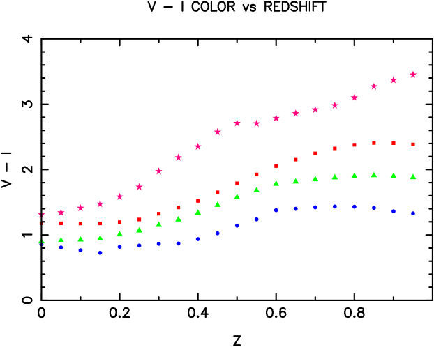
Figure 5: Galaxy color vs redshift for the UH8K system and using broad band SED’s from ?) . Symbols encode the galaxy type as follows: E0 = stars; Scd = squares; Sbc = triangles; Im = circles.

3.3 Bright Galaxy Properties and Cluster Luminosities

We will now explore the properties of the brighter galaxies which define the supercluster and estimate the optical luminosities of the clusters. In the absence of redshift information this is rather difficult because of the presence of foreground structures. We can however obtain fairly accurate estimates of the individual cluster luminosities for the early-type cluster galaxies as the noise due to foreground and background contamination is then greatly reduced.

In figure 6 we plot the locations, colors, and fluxes of the bright galaxies in the field. At the center of each circle drawn around the X-ray positions resides a dense concentration of very red galaxies with colors as expected for elliptical galaxies at $z=0.42$. In addition to the red elliptical galaxies, a large number of bluer and brighter galaxies can be seen. One conspicuous concentration lies $2^{\prime}-3^{\prime}$ to the East of CL-N, and, to judge from the colors and fluxes of the galaxies, lies at $z\simeq 0.2$. Another, more diffuse concentration, with colors and luminosities indicative of early type galaxies at $z\simeq 0.3$ can be seen extending Westward of CL-S. We have obtained redshifts for two of the bright galaxies in this complex and find that they do indeed lie at $z\simeq 0.3$.

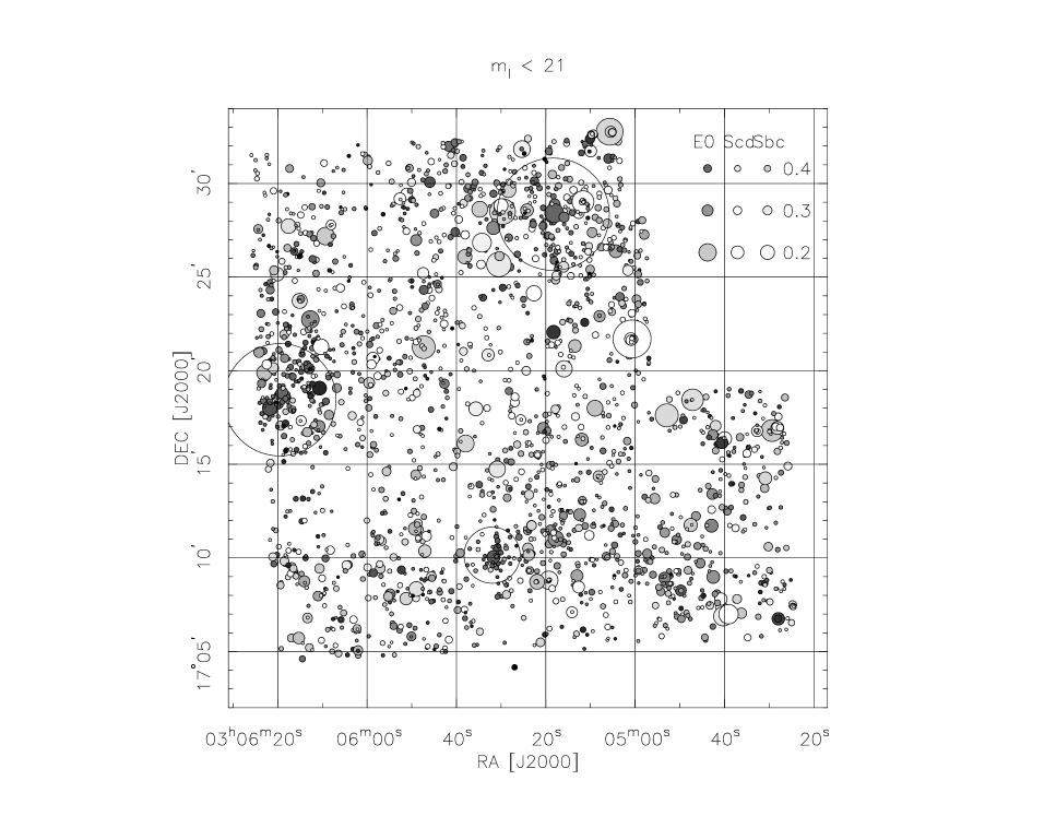
Figure 6: Plot of all galaxies brighter than $I=21$ where the area of each circle is proportional to the flux density of the galaxy, and the shade of the disc encodes the $V-I$ color, ranging from $V-I=1$ for a white disc to $V-I=3$ for a black disc. The legend in the upper right corner shows the image that would be produced by an $L_{*}$ galaxy ($M_{B}=-19.68$) of various types at redshifts $0.2,0.3,0.4$. Stars have been removed. The three main galaxy concentrations are apparent, as is an extension to the West from southern EMSS cluster. The large circles have radius $3^{\prime}$ ($1^{\prime}.5$ for CL-S) and are centered on the X-ray cluster positions.

We can obtain an unbiased, if somewhat noisy, estimate of the abundance of galaxies in general in the three X-ray clusters by computing the counts of all galaxies (the number of galaxies per solid angle per magnitude interval) within the cluster-centered circles and then subtracting the ‘background’ counts obtained for the complementary region. The counts as a function of $I$-band apparent magnitude are shown in figure 7. In computing the counts we allow for the somewhat irregular survey geometry caused by our masking of bright stars (the mask is shown below in figure 11). To estimate the unmasked areas we count the number of objects from a densely sampled random Poissonian distribution of points which was masked in exactly the same way as the galaxy catalogs. The error bars in figure 11 are poissonian only, and the real fluctuations are somewhat larger. The excess of galaxy counts due to the clusters is clearly visible. Similar results are obtained for the synthetic rest-frame $B$-magnitude $m_{B_{z}}\simeq(m_{I}+m_{V})/2$, though these start to become incomplete at somewhat brighter magnitudes.

Figure 7: Counts of galaxies for the ‘cluster’ regions defined by the circles in figure 6, and for the complementary region.

The color magnitude diagrams shown in figure 8 reveal a distinct excess of galaxies in a narrow band of color around $V-I=2.2$ in the cluster regions, as predicted for early type galaxies at $z=0.42$ from figure 5. By selecting only galaxies within a narrow strip in color-magnitude space straddling this sequence we can obtain fairly precise estimates of the early-type luminosity functions for the three clusters, and for the clusters taken together, since the fluctuations in the background estimates are greatly reduced. The results are shown in figure 9 where we plot the spatial distribution of galaxies in a $\simeq 0.5$ mag wide strip (corresponding to a range of redshifts $\Delta z\simeq 0.1$) and in figure10 where we plot the excess counts of the color selected galaxies (corrected for field contamination) $\Delta N=A_{c}\times(n_{c}-n_{f})$, where $A_{c}$ is the area of the cluster circles, as a function of $M_{B}=m_{I^{\prime}}-c_{I^{\prime}}+c_{B}+k_{BI^{\prime}}(z=0.42)-{\rm DM}(z)$. Also shown is the luminosity function of form similar to those found by ?) and ?): $\Phi(L_{B})=\Phi_{*}(L/L_{*})^{\alpha}\exp(-L/L_{*})$ with $M_{*}=-19.68$ and $\alpha=-1.0$ and with amplitude $\Phi_{*}$ scaled to fit the counts. This standard, low-redshift, field galaxy luminosity function seems to provide a reasonable fit to the cluster count excess down to magnitudes well below the knee, and so integrating the luminosity functions should give a good estimate of the total red cluster light.

To obtain estimates for the individual cluster luminosities we fit the excess counts to the form above to determine $\Phi_{*}$ as

$$\Phi_{*}=\sum\Delta Nf(M_{B})/\sigma^{2}/\sum f(M_{B})^{2}/\sigma^{2}$$ (6)

where $f(M_{B})=(L/L_{*})^{1-\alpha}\exp(-L/L_{*})$ and $\sigma$ is the rms fluctuation in $\Delta N$ due to Poisson counting statistics. We then integrate the luminosity functions to obtain the total excess luminosities within the circles defining the cluster subsample. These are tabulated in table 2. These luminosity functions are only for the color selected subsample. Performing the same exercise to compute the total luminosity function using our synthetic $B$-band magnitudes we find noisier results, but conclude that about 70% of the total excess light within our cluster apertures comes from early type galaxies, in rough agreement with ?) who found that about 25% of the galaxies in CL-N for instance were blue with ‘Balmer-line’ spectra.

Figure 8: Color-magnitude diagrams for the cluster and field subsamples.

cluster	$\phi_{*}$	$L/L_{*}$	$h^{2}L/L_{\odot}$
E+N+S	59.27	128.70	1.49e+12
CL-S	6.34	13.77	1.60e+11
CL-E	30.30	65.81	7.63e+11
CL-N	17.87	38.81	4.50e+11

Table 2: Table of cluster luminosities.

Figure 9: Early type galaxy sample. The spatial distribution of galaxies with colors $1.9<V-I<2.4$ and $I<23$ chosen to select early type galaxies at around the redshift of the super-cluster. The area of each circle is proportional to the flux. The range of colors here corresponds to a depth $\Delta z\simeq 0.1$, so we would expect to find a substantial contamination by ‘field’ galaxies in addition to the super-cluster galaxies.

Figure 10: Rest frame $B$-band luminosity functions for the three X-ray clusters and for the three clusters combined. The counts here have been corrected for field contamination and the lines are fits to a Schechter function with $M_{*}$, $\alpha$ fixed at the values obtained for low redshift field samples.

The standard definition of cluster richness Abell (1958) is the number of cluster galaxies in the range two magnitudes below the third brightest, with richness class $R=1$ corresponding to 50-80 galaxies etc. It is clear from inspection of figure 10 that these clusters are not very rich by this measure. Both CL-N, CL-E are borderline richness class 1 and CL-S is a very poor cluster.

The southern cluster CL-S is particularly compact; most of the elliptical galaxies lie within about $1^{\prime}$ (or about $200h^{-1}$kpc) of the X-ray location. This is almost an order of magnitude smaller than the conventional Abell radius of $1500h^{-1}$kpc. This is consistent with the compact X-ray appearance for this cluster, but also somewhat surprising. According to the standard hierarchical clustering picture, clusters which turn around and virialize at time $t$ have a density $\sim 170$ times the critical density at that age: $\rho\sim 170\rho_{\rm crit}(t)=170/(6\pi Gt^{2})$. With $r\simeq R_{\rm Abell}$ and $\sigma\simeq 1000$km/s, as typical of massive clusters, we obtain a collapse time $t\simeq 10^{10}h^{-1}$yrs, similar to the present age of the universe and therefore in reasonable agreement with the theoretical expectation. With $\sigma=920$km/s and $r\simeq 200h^{-1}$kpc however, we obtain a collapse time $t\simeq 2\times 10^{9}$yr, which is much less than the age of the universe at $z=0.42$. If this cluster is virialized and did indeed form by something like the spherical collapse model then it did so a very long time ago at $z\sim 3-5$ and little visible matter has accreted onto it since then.

4 Shear Analysis

4.1 Background Galaxy Selection and Shear Measurement

We now describe how we select the faint galaxies which we use for measuring the shear, how we correct for psf anisotropy and calibrate the effect of seeing. We also describe how we construct a weighting scheme to combine the signal from galaxies of a range of sizes and luminosities to give a reconstruction with optimal signal to noise.

Stars are easily visible to $m_{I}\simeq 23$ (figure 4) and we remove these and also the tail of faint objects with estimates half-light radii less than $0.3^{\prime\prime}$. Some close pairs of galaxies get detected as single objects, and these were filtered by applying a cut in ellipticity (see below) which we set at $e=0.7$. To obtain a sample which is distant and minimally contaminated by cluster galaxies we make a cut at $\nu=100$ to remove bright objects. The resulting catalog contains about $30,000$ objects, with a surface density of about $50$ per square arcmin. The spatial distribution of this faint galaxy sample is shown in figure 11, which confirms that they are very uniformly distributed across the field.

Figure 11: Spatial distribution of the faint galaxy sample. They are clearly distributed very uniformly across the sky as one would expect if they are very distant. The rectangles were placed to mask out diffraction spikes and trails from bright stars.

The shear measurement is described in more detail elsewhere Kaiser (1988). It is similar in spirit to the ?) analysis in that we compute response functions which tell us how the shape statistics respond to psf anisotropy and to gravitational shear. The fundamental shape statistic we use is the flux normalized weighted second central moment of the measured surface brightness $f(r)$:

$$q_{lm}={\int d^{2}rr_{l}r_{m}w(r)f(r)\over\int d^{2}rf(r)}$$ (7)

where $w(r)$ is a Gaussian profile weight function with scale matched to the size of the object. KSB computed the response of the ellipticity or ‘polarization’ defined as $e_{\alpha}\equiv M_{\alpha lm}q_{lm}/q_{pp}$, where the pair of $2\times 2$ matrices are $M_{0}=\{\{1,0\},\{0,-1\}\}$, $M_{1}=\{\{0,1\},\{1,0\}\}$, to both psf anisotropies and, in the limit of well resolved galaxies, to gravitational shear. ?) generalized this to obtain the post-seeing shear response function $P_{\gamma}$ such that $\langle e_{\alpha}\rangle=\gamma_{\alpha}P_{\gamma}$ and which serves to calibrate the relation between the observable polarization and the gravitational shear $\gamma_{\alpha}=(1/2)M_{\alpha lm}\Phi_{lm}$ where $\Phi_{lm}$ is the projected gravitational potential.

In ?) the psf anisotropy was modeled as a low order polynomial in position on the image. Such a model is not adequate for observations such as those considered here taken with a mosaic camera where one finds that the psf varies smoothly across each chip, but changes discontinuously as one passes across chip boundaries resulting in a complicated pattern of psf anisotropies on the final averaged image. Since we know which source images contribute to a given galaxy image, we can compute an average of the psf anisotropy response function measured from the individual images modeling these as a smooth polynomial functions over each of the source images. This would not be quite correct however, since the response function for the ellipticity, which is a non-linear function of the surface brightness, is itself non-linear, so the averaged response function does not, in general, correctly describe the response of an averaged galaxy image. What we do instead is to compute the response functions for the flux normalized $q_{lm}$ moments themselves. Since psf anisotropy does not affect the net flux appearing in the denominator (we assume that our fluxes are effectively total fluxes), the psf response is a linear function of the sky brightness $f(r)$ and can therefore be averaged to give the correct response for the $q_{lm}$ which we use to correct the $q_{lm}$ values to what would have been measured by a telescope with a psf of same size and overall radial profile as the real psf but with no anisotropy. We then form a polarization $e_{\alpha}$ as above from the anisotropy-corrected moments, and compute the post-seeing shear response function $P^{\gamma}$, such that, on average, the polarization $e_{\alpha}$ induced by a gravitational shear $\gamma_{\alpha}$ is

$$\langle e_{\alpha}\rangle=P^{\gamma}\gamma_{\alpha}$$ (8)

We do not attempt to calibrate the galaxies individually; this tends to be noisy and introduces non-linear effects. Instead we split the galaxies up into a set of discrete subsets by a coarse binning in the significance - half light radius plane $(\nu,r_{h})$, and compute an average $P^{\gamma}$ for all the galaxies in each bin and thereby compute shear estimates $\hat{\gamma}_{\alpha}=e_{\alpha}/\langle P_{\gamma}\rangle$. Having split the galaxies up into classes by size and magnitude in this way we can then compute an optimal weight as a function of the bin. To do this we assume that all of the galaxies are at large, or at least similar, distance from the lens and therefore feel essentially the same shear, and also that the shear signal is much less that the random shear noise due to intrinsic shape and measurement errors combined. We compute the variance in shear estimates $\langle\gamma_{\rm noise}^{2}\rangle\simeq\langle e^{2}\rangle/\langle P_{\gamma}\rangle^{2}$ for each bin and assign weights inversely proportional to the variance and such that the sum over galaxies of the weights is equal to the number of galaxies (so the result is unbiased). With this scheme, faint and/or very small galaxies which are relatively noisy get assigned lower weights.

In figure 12 we show the distribution of weight in the size magnitude plane and we also show the distribution of weight as a function of magnitude. The rms shear (per component) in the final catalog is $\sigma_{\gamma}\simeq 0.32$ so we should be able to measure shear to a high precision. For instance, for measurement of the net shear we expect the precision to be $\sigma_{\gamma}/\sqrt{N_{\rm gals}}\simeq 0.002$

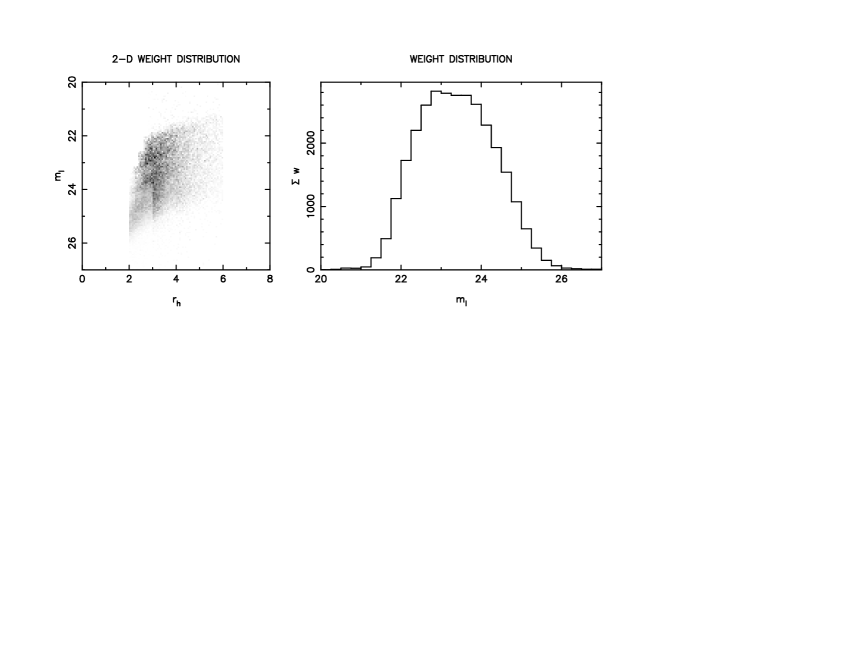
Figure 12: Left panel shows the distribution of weight as a function of size and magnitude. The edges of the coarse bins can be seen as discontinuities in the weight density. Right panel shows the distribution as a function of magnitude. Roughly half of our weight comes from galaxies brighter than $m_{I}=23.5$, where the redshift distribution is fairly well established Cowie et al. (1996), but half comes from fainter magnitudes where there is only very poor sampling as yet.

The largely unknown redshift distribution for galaxies at this range of magnitudes and sizes is a major source of systematic uncertainty in weak lensing mass estimation. For $m_{I}\lesssim 23$ there are reasonably complete statistical samples Cowie et al. (1996) but at fainter magnitudes things become progressively uncertain. For sources at a single redshift $z_{s}$, the dimensionless surface density $\kappa$ that we measure for a lens of physical mass surface density $\Sigma_{m}$ is $\kappa=\Sigma_{m}/\Sigma_{\rm crit}(z_{s})$ where

$$\Sigma_{\rm crit}={c^{2}\over 4\pi GD_{l}}{D_{s}\over D_{ls}}\equiv\Sigma_{\rm crit}^{\infty}\beta^{-1}$$ (9)

where $D_{ls}$ is the angular diameter distance relating physical distance on the source plane to angles at the lens and where the factor $\beta\equiv D_{ls}/D_{s}$ is the distortion strength relative to that of sources at infinite distance. With sources at a range of distances what we measure is the physical surface density times an average inverse critical density, or $\kappa=(\Sigma_{m}/\Sigma_{\rm crit}^{\infty})\langle\beta\rangle$. The critical surface density and the $\beta$ parameter are shown, for a lens redshift $z_{l}=0.42$ in figure 13.

Figure 13: Left panel shows the inverse critical surface density as a function of source redshift for a lens at $z_{l}=0.42$. The physical surface density of a lens is obtained by dividing $\kappa$ by a weighted average inverse critical surface density taken over the distribution of background galaxies. The panel on the right shows the $\beta$ parameter; for a lens of given velocity dispersion, X-ray temperature, the predicted shear is proportional to $\beta$. The three lines are for EdS (solid), empty open (dot-dash) and $\Lambda$ dominated cosmology (dotted).

Using the photometric redshifts in the Hubble Deep Field from Sawicki et al. (1997) and assuming an empty open universe gives $\langle\beta\rangle\simeq 0.46$. Using an alternative, and more recent, HDF photo-z catalog calculated Fern’andez-Soto et al. (1998) we find similar results. Both catalogs contain about 1000 galaxies. The $\langle\beta\rangle$ value was calculated by transforming HDF $I_{\rm F814W}$ AB magnitudes to Cousins $I$-band magnitudes according to the WFPC2 Handbook and HDF web-page, and corresponds to that for a single screen of background galaxies at $z_{s}\simeq 1.0$.

There is considerable uncertainty in this value. There are some questions about the reliability of photometric redshifts, the calculation above does not incorporate the weighting as a function of size, and the cosmological background model may be inappropriate. Another result which casts some doubt on the detailed accuracy of the distribution of photometric redshifts is that they are somewhat hard to reconcile with weak lensing results for $z\simeq 1$ clusters (Luppino & Kaiser (1997); Clowe et al. (1998)). In what follows we shall adopt a value of $\Sigma_{\rm crit}=4.33\times 10^{15}hM_{\odot}/{\rm Mpc}^{3}$, slightly higher than that derived from the photometric redshifts, and corresponding to a single screen redshift of $z_{s}\simeq 1.5,\;1.2;0.75$ for EdS, empty open and $\Lambda$ dominated cosmologies respectively.

4.2 Predicted Dimensionless Surface Density

We now compute the dimensionless surface density $\kappa$ that would be generated by the optical structures assuming that galaxies are good tracers of the total mass with some constant mass-to-light ratio We know of course that on mass scales of the order of tens of kpc the dark matter distribution is much more extended than the light, but on larger scales this ‘what you see is what you get’ picture remains an interesting and viable hypothesis.

If all of the structures lay at the same lens-redshift $z_{l}$ this would be straightforward since we then have

$$\kappa\equiv{\Sigma_{\rho}\over\Sigma_{\rm crit}}=(M/L)\Sigma_{l}/\Sigma_{\rm crit}(z_{l})$$ (10)

where $\Sigma_{l}$ is the rest frame luminosity surface density, which we can compute from the observed surface brightness.

This would be adequate to compute the contribution just from the $z=0.42$ supercluster, but, as we have seen, there are other structures at different redshifts that we would like to include, and one cannot then use this simple procedure because it would cause one to grossly overestimate the effect of foreground structures. This is because, for a lens with given rest-frame surface luminosity and mass surface density, the observed surface brightness falls very rapidly with increasing lens redshift (roughly as $(1+z)^{-4}$ but with an extra decrease for early type galaxies which tend to have $\lambda f_{\lambda}$ increasing with $\lambda$) while the dimensionless surface density $\kappa\propto 1/\Sigma_{\rm crit}$ is a strongly increasing function of lens redshift for $z_{l}\ll z_{s}$. These trends are quantified in figure 14. For early type galaxies, and in the $I$-band, the ratio of $\Sigma_{l}/\kappa$ falls by about a factor of 3 as the lens redshift is varied from 0.2 to 0.4. Note also that high redshift clusters, if they exist, could give quite a strong lensing effect while being relatively inconspicuous in photometric surveys (the $\kappa$ curve is rather flat, while the $\Sigma_{l,{\rm obs}}$ curve plunges rapidly). For example, a cluster at redshift unity produces a shear per surface brightness about one order of magnitude larger than the same cluster at redshift $0.42$ (this is neglecting the evolution of the cluster galaxies which tends to act in the opposite direction).

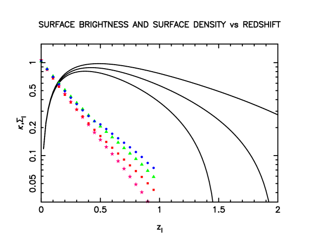
Figure 14: The filled symbols show the observer-frame surface brightness (in the UH8K $I$-band) of a cluster lens as a function of lens redshift and for various galaxy types, assuming no evolution in the rest-frame surface brightness. Symbols encode the galaxy type as follows: E0 = stars; Scd = squares; Sbc = triangles; Im = circles. The lines show the inverse critical surface density, which for a lens of a given physical surface density density, is proportional to the observed dimensionless surface density $\kappa$, for sources at redshifts $z_{s}=(1.5,2.0,3.0)$.

To make an accurate prediction for the dimensionless surface density $\kappa$ then, it is not sufficient just to use the net surface brightness; one needs some idea of the distances to the galaxies. Ideally, one would obtain redshifts for all of the bright galaxies and then one could correctly account for this, but as yet we do not have this information. A solution to this problem is suggested by figure 5. If we only use galaxies redder than $V-I\simeq 1.6$ then we should see elliptical galaxies at $z\gtrsim 0.2$, and later type galaxies only at $z\gtrsim 0.4$. For an elliptical galaxy, we can read off the redshift from the color using figure 5 (we model the color-redshift relation as a linear trend fixed by the values at $z=0.2$ and $z=0.4$). We can then compute the physical luminosity, and thereby the mass (assuming a constant $M/L$), and thereby compute it’s contribution to the $\kappa$ field. For a single galaxy with observed magnitude $m$, and for an EdS cosmology, the contribution to an image of $\kappa$ from a galaxy which falls in a pixel with solid angle $d\Omega$ is

$$\kappa d\Omega={M\over L}{4\pi GM_{\odot}a_{0}\over c^{2}(10{\rm pc})^{2}}(1+z)^{3}{\omega_{l}\omega_{ls}\over\omega_{s}}10^{0.4(M_{B\odot}-m-k(z))}$$ (11)

where $M/L$ is in solar units and $\omega=1=1/\sqrt{1+z_{l}}$.

If we generate a surface density prediction $\kappa$ in this manner we will, to a very good approximation have isolated the contribution from the early type galaxies at $z\gtrsim 0.2$ alone. To see why, consider first the blue galaxies associated with the clusters at $z\simeq 0.42$, which we have seen contribute at most about 30% of the cluster $B$-band light. Some fraction of these — the very reddest — will survive the color limit of $V-I=1.6$, but by the above prescription they will be assigned a redshift of $\sim 0.2$, rather than their actual redshift of $0.42$ and so their contribution to $\kappa$ as calculated above will be suppressed in proportion to the lens redshift dependent factors in equation (11): $(1+z)^{3}\omega_{l}(z_{l})\omega_{ls}(z_{l},z_{s})10^{-0.4k(z_{l})}$ or about a factor 6 in this example, so, even if we assume that say 30% survive the color selection, the contribution to $\kappa$ will only be about $1/20$ of the true contribution of all the blue galaxies, or about $1/60$ of the contribution of the elliptical galaxies. At higher redshift a larger fraction of later type galaxies survive the color selection, but for these the contribution to $\kappa$ will be suppressed by an even larger factor. Moreover, these galaxies are found to be very nearly uniformly distributed on the sky; thus their contribution to the fluctuating part of $\kappa$ — which is entirely responsible for the shear we are trying to predict — is expected to be very small and it should be safe to neglect them as compared to the early type galaxies at lower redshift. Also, our linear extrapolation of the color-redshift relation exceeds the actual predicted colors for $z\gtrsim 0.6$, and this effectively suppresses the contribution from higher redshifts.

With this color-based redshift estimation we obtain a prediction for $\kappa$ which will be correct if early type galaxies trace the mass with some constant $M/L$, (though missing some or all of the contribution from very distant structures where our selection function cuts off around $L_{*}$ or brighter). We should stress that this is a rather unconventional hypothesis. The general picture of the structure of superclusters, supported by the ?) morphology density relation, galaxy correlation functions Loveday et al. (1995) and studies of individual structures like the Virgo Supercluster, is of the elliptical galaxies residing in dense compact clusters, with the later type galaxies (which dominate the total luminosity) being much more extended. If this supercluster conforms to the norm, then the mass should be more extended than the early type galaxies and we should see this in the gravitational shear field, and if one incorporates statistical ‘biasing’ (e.g. Bardeen et al. (1986)) then the mass would be expected to be still more extended.

The resulting predicted $\kappa$ field smoothed with a Gaussian kernel of scale length $31^{\prime\prime}$ is shown in figure 15. We show both the $\kappa$ just due to the $z\simeq 0.42$ cluster galaxies and also for a broader color selection. These were made with $M/L=200h$ which, as we shall see, is similar to the value preferred by our shear measurements. The differences are not large, though there is some contribution from the structure extending West from CL-S which lie at $z\simeq 0.3$, and there are several other weaker features.

The luminosity density field we measure is obtained from fluxes measured within apertures around the galaxies (these were taken to be three times the Gaussian scale length of the detection filter) and so will differ slightly from the total luminosity dependence because of two competing effects; the apertures are finite and so miss some of the light, but also sometimes overlap so that light gets double counted. To test how large the net bias is we have made estimates of the total extra-galactic surface brightness field in two ways: by summing the fluxes from the catalog and by using all the light in an image from which we have masked out all the stars. The results agree to better than 10 percent, so we conclude that we are measuring essentially the total luminosity.

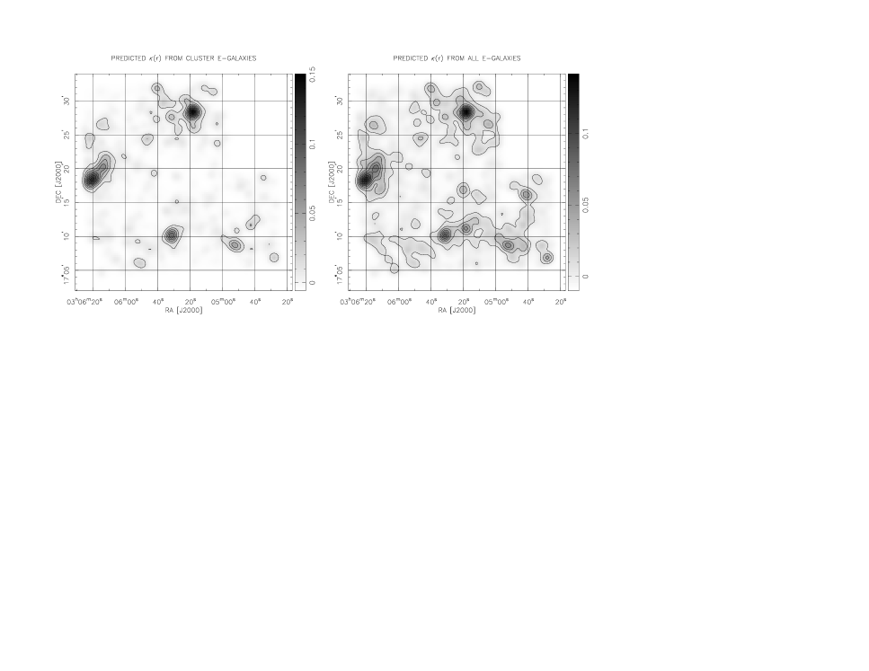
Figure 15: Predicted dimensionless surface density $\kappa$. Images have been smoothed with a $31^{\prime\prime}$ arcmin Gaussian low pass filter. The mean has been subtracted from each image. The left panel shows the predicted $\kappa$ only from galaxies in a narrow band of color around $V-I\simeq 2.2$ for elliptical galaxies $z=0.42$. The right hand panel shows the results for all galaxies redder than $V-I=1.6$ and with contribution given by equation 11.

4.3 Predicted and Observed Shear

Armed with the predicted $\kappa(r)$ from the previous section we can compute the shear field and compare with what we observe. To generate the predicted shear from the $\kappa$ images we solve the 2-dimensional Poisson’s equation by FFT techniques (padding the predicted $\kappa$ image out to twice its original size with zeros to suppress the effect of periodic boundary conditions) to obtain the surface potential $\Phi$, and then differentiate this to compute the shear $\gamma_{\alpha}=M_{\alpha lm}\Phi_{lm}/2$. This provides us with an image of the shear field, and with this we can generate for each galaxy in our faint galaxy catalog the value of the predicted shear, and we can then ask, for instance, what is the multiple of the predicted shear which, when subtracted from the observed shear minimizes the summed squared residuals. We can also bin the galaxies according to predicted shear — here we treat the two components of the shear for each galaxy as independent measurements — and plot the average measured shear versus that predicted. To minimize the effect of shear generated by structures outside the field in this analysis, we subtract, from both the observed and predicted shears, the mean shear.

If we assume that light traces mass and that the errors are predominantly in the shear measurement then to obtain the mass-to-light ratio we should compute $\alpha=\sum\gamma^{\rm obs}\cdot\gamma^{\rm pred}/\sum\gamma^{\rm pred}\cdot\gamma^{\rm pred}$, and then multiply this by our nominal value to obtain $M/L_{B}=200h\alpha$. We find $\alpha=1.20$, with this value giving a reduction in $\chi^{2}\equiv\sum(\gamma-\gamma_{\rm model})^{2}/\sigma_{\gamma}^{2}$ of $79$ relative to the value for $\alpha=0$, from which we infer $M/L_{B}\simeq 240h$. The correlation between the predicted and observed shear is shown in figure 16 and is significant at about the $\sim 10$-sigma level.

Figure 16: Predicted vs observed shear assuming $M/L_{B}=200h$. Error estimates were obtained from an ensemble of catalogs with randomized shear values.

A weakness of this method is that the light was smoothed, whereas the shear values are unsmoothed. If light really traces mass fairly on all scales, then this would cause our estimate to underestimate the true mass to light ratio by a factor $\int d^{2}kP(k)\omega(k)^{2}/\int d^{2}kP(k)\omega(k)$ where $\omega(k)$ is the smoothing filter and $P(\omega)$ is the luminosity power spectrum. If mass were distributed around galaxies in halos of shape proportional to $\omega(r)$, however, then we would obtain the correct $M/L$. Conversely, if it were the case that the dark matter distribution is more extended than our smoothing filter then we will have underestimated the global $M/L$. We will return to this issue shortly.

4.4 2-D Surface Density Reconstruction

We now show 2-D mass-reconstructions and compare with the projected luminosity density. We will also compare the results obtained using the $V$- and $I$-band observations separately, and with the level of noise expected due to the random intrinsic galaxy shapes. We use the ?) reconstruction algorithm. This is a stable and fast reconstruction method which has very simply defined noise properties; essentially Gaussian white noise. Its main drawbacks are that it does not properly account for patchy data and the finite data boundaries. We have found from simulations that the former is not a serious problem for these data, but the latter is worrying, particularly for cluster CL-E, which lies right at the edge of the field and so some of the shear signal is lost, resulting in a suppression of the recovered mass. To get around this we proceed as follows: first we make a shear field image prediction from the constant $M/L$ $\kappa$ prediction. We then sample this at the actual positions of our faint galaxies to generate a synthetic catalog (that which would have been observed with no intrinsic random shape or measurement noise), and then generate a reconstruction from that synthetic catalog which will have the same finite-field bias as the real reconstructions. To match the spatial resolution to that of the real reconstructions (a $45^{\prime\prime}$ Gaussian) we make the predicted shear with a smoothing scale $45^{\prime\prime}/\sqrt{2}$ and make the reconstruction from the synthetic catalog with the same smoothing. Note that while correctly accounting for the finite field effect on structures within the field, the actual shear may still feel some effect from structures outside of the field.

In figure 17 we show the mass reconstruction from our combined faint galaxy sample on the left and that predicted (for a nominal $M/L_{B}=200h$) on the right. There is generally quite good agreement between the mass and the light. All three of the main $z\simeq 0.42$ clusters are clearly detected in the reconstruction, and the locations of these peaks coincide very accurately. We see no obvious indication that the mass in these clusters is more extended than the elliptical galaxy light. The lower redshift structure extending to the South-West of CL-S is also recovered in our reconstructions. There is some indication of a ‘bridge’ linking CL-S, CL-N, which is suggestive of the kind of features predicted by the ‘cosmic-web’ theory Bond et al. (1996). Part of this bridge is a clump at $\alpha\simeq 3^{h}05^{m}15^{\prime\prime}$, $\delta\simeq 17^{\circ}16^{\prime}$ which roughly matches a predicted, though somewhat weaker, feature. However, this is not at the supercluster redshift, and so part of the ‘bridge’ may be a coincidental projection. There is a rather conspicuous mass clump around $\alpha\simeq 3^{h}05^{m}57^{\prime\prime}$, $\delta\simeq 17^{\circ}14^{\prime}$ which has no apparent counterpart in the predicted field.

There is considerable noise in the reconstructions. The noise power spectrum is white, while the galaxy power spectrum is relatively red, so we might expect to see better agreement if we further smooth both the light and mass maps, and to this end we show in the lower pair of panels of figure 17 the results for a smoothing scale of $\simeq 90^{\prime\prime}$.

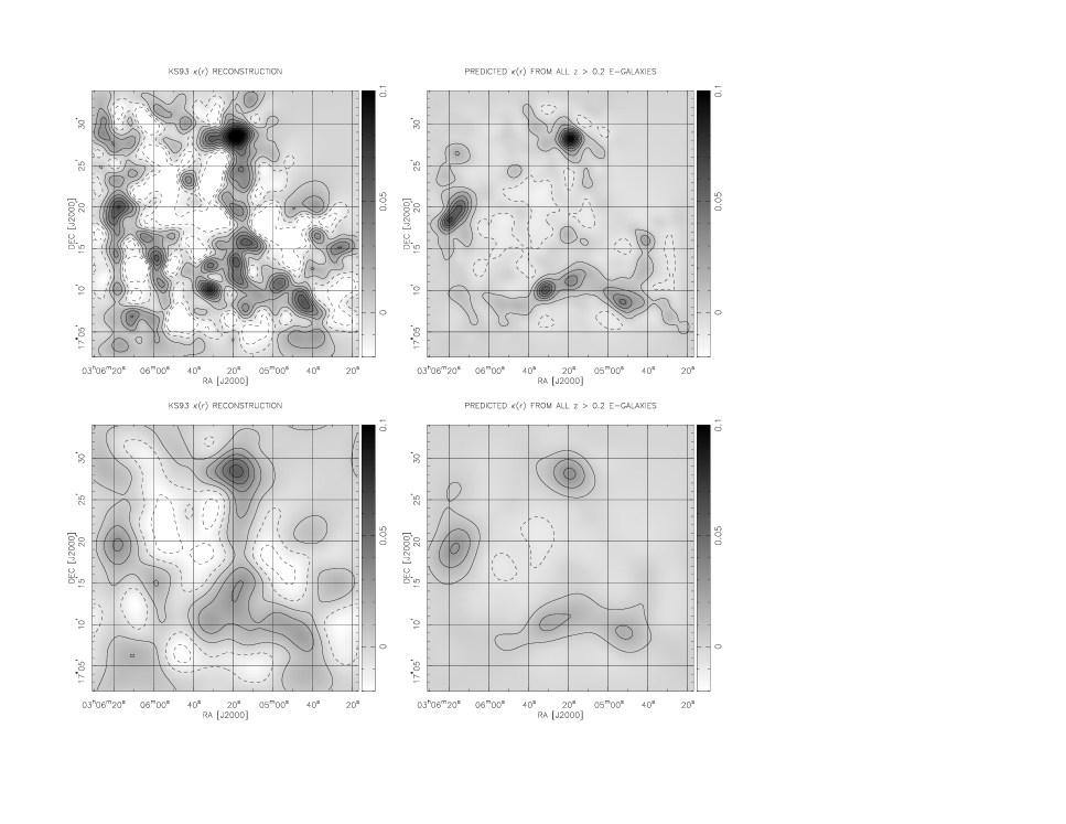
Figure 17: Left panel shows the recovered mass using the ?) reconstruction method. Right panel shows the predicted 2-D reconstruction using the shear predicted from the light-map (but sampled at the actual locations of the faint galaxies) which should have the same finite field biases as the real reconstructions. The lower panels show the same images smoothed with a Gaussian of scale $90^{\prime\prime}$

Figure 18 shows mass reconstructions made from the I-band and V-band observations separately. These show generally very good agreement, with most of the features described above being visible in both images. The anomalous ‘dark clump’ lying between CL-S and CL-E is however not very evident in the $V$-band reconstruction. Also shown is a reconstruction obtained using a catalog with the real faint galaxy positions but with the measured shear values shuffled (i.e. reassigned to the galaxies in random order). The fluctuations in this random reconstruction show the expected noise level due to random intrinsic ellipticities. We have made an ensemble of 32 such realizations and we use these below to quantify the significance of our results.

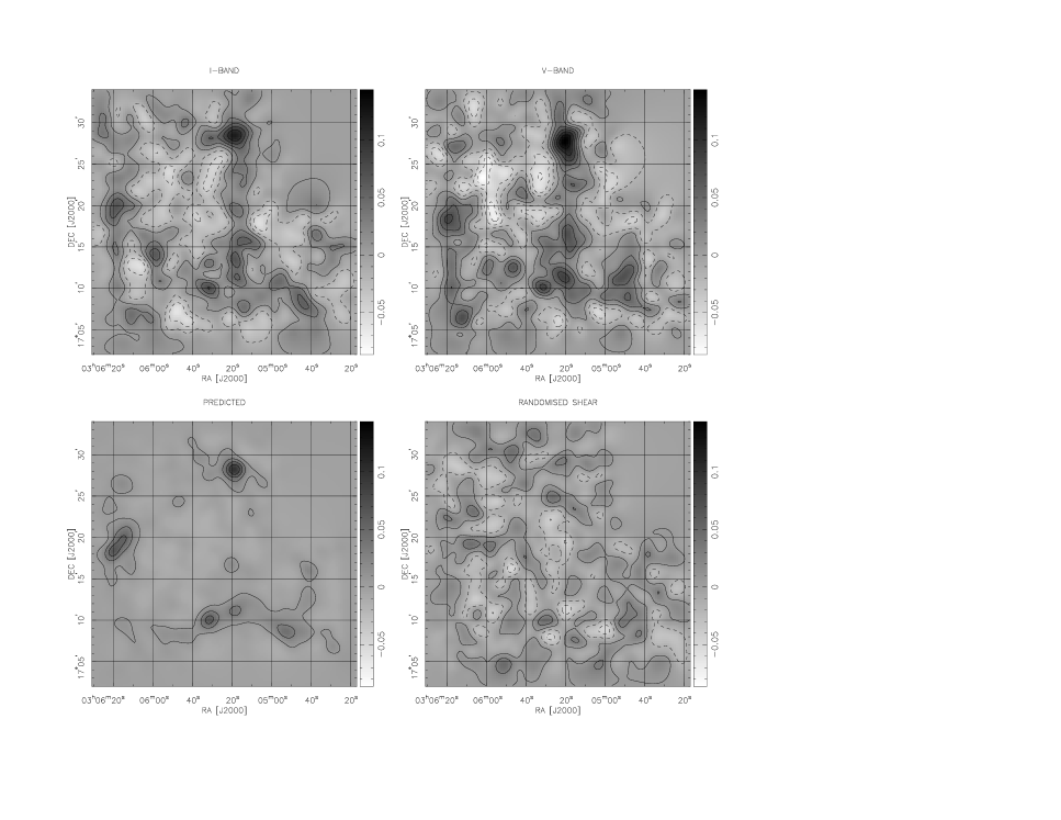
Figure 18: Upper panels show the reconstructions from catalogs made from the $I$ and $V$ band images separately and show generally very good agreement. Lower left panel shows the early-galaxy $M/L=200h$ prediction. Lower right panel shows the reconstruction from a catalog with randomized ellipticities, which indicate the expected noise fluctuations due to intrinsic random galaxy shapes.

4.5 Cluster Masses and Mass to Light Ratio’s

We now estimate the masses of the three $z\simeq 0.42$ clusters. We will use these to derive mass-to-light ratios, and also to compare with independent mass estimates from the X-ray temperature and velocity dispersions. We compute the masses within circular apertures of radius $1^{\prime}.5$ and $3^{\prime}.0$ from the reconstructions (which have been smoothed with a $45^{\prime\prime}$ Gaussian), and we estimate mass-to-light ratios by dividing the mass by the predicted mass within the same apertures. Thus, the $M/L$’s we obtain should be corrected for finite field effects. The results are tabulated in table 3.

cluster	$r_{\rm{ap}}$/arcmin	$\overline{\kappa}$	$\nu$	$h^{-1}M/L$	$hM/10^{12}M_{\odot}$
CL-S	$1.5$	$0.0318\pm 0.0096$	$3.3$	$241\pm 72$	$37.9\pm 11.4$
CL-E	$1.5$	$0.0455\pm 0.0164$	$2.8$	$182\pm 65$	$54.2\pm 19.6$
CL-N	$1.5$	$0.0758\pm 0.0100$	$7.6$	$342\pm 44$	$90.5\pm 11.9$
E+N+S	$1.5$	$0.1586\pm 0.0234$	$6.8$	$263\pm 38$	$189.1\pm 27.9$
CL-S	$3.0$	$0.0131\pm 0.0066$	$2.0$	$296\pm 149$	$62.4\pm 31.5$
CL-E	$3.0$	$0.0206\pm 0.0065$	$3.1$	$193\pm 61$	$98.1\pm 31.2$
CL-N	$3.0$	$0.0434\pm 0.0081$	$5.3$	$466\pm 87$	$206.9\pm 38.7$
E+N+S	$3.0$	$0.0764\pm 0.0140$	$5.4$	$314\pm 57$	$364.7\pm 66.9$

Table 3: Cluster masses and mass to light ratios. The mean dimensionless surface density $\overline{\kappa}$, the mass $M$, and the mass to light ratio have been corrected for finite field effects. The $\nu$ value is the significance of the measurement determined by comparing with the rms mass measured for the ensemble of randomised catalogs.

Table 3 shows an increase in $M/L$ with aperture radius for all three clusters. For CL-E, CL-S, this is slight and not particularly significant. For CL-N the increase is larger, but we caution that there is a foreground cluster which lies just to the East of CL-N and which falls within the larger aperture. While we have argued above that there should in general be a rather weak contribution from low redshift structures, in this case the foreground cluster is particularly bright, and so may contribute significantly to the increase in $M/L$ for CL-N. Redshift information is needed to properly quantify this. We note that these $M/L$ values, averaging around $260h$ for our $1^{\prime}.5$ apertures (which give the highest signal to noise for $M/L$) are much lower than has been found for other, generally more massive, clusters like A1689 Fischer & Tyson (1997). In so far as only a tiny fraction of the Universe resides in such super-rich systems, it may well be that the value obtained here is more representative. It is also interesting to note that these $M/L$’s only include the contribution from early type galaxy light in a rather narrow band of color. CL-N was found by ?) to contain a number of bluer ‘Balmer-line’ galaxies, about $\sim 25$% of the total, which would bring the total $M/L$ is more in line with that for CL-S, which they found to be almost entirely early galaxy dominated.

It is of interest to compare these masses with those obtained from the CL-S temperature and with velocity dispersions for all 3 clusters. For CL-S, our mass is in good agreement with the X-ray mass (which in turn is in good agreement with the velocity dispersion). For CL-N, we model the galaxies as an isothermal gas with profile index $d\log n/d\log r\simeq-1.5$ as measured from the observed counts profile to find a predicted $\overline{\kappa}\simeq 0.93$ (for the $1^{\prime}.5$ aperture) as compared to the measured value $\overline{\kappa}=0.076\pm 0.01$, again in reasonably good agreement given the statistical and systematic modeling uncertainties. For CL-E the same exercise gives a predicted surface density about a factor two higher than what we measure, but this may be due to departures from assumed equilibrium in this clearly non-relaxed system.

4.6 Light-Mass Cross-Correlation

In this section we show the results of cross-correlating the mass and the light. Our goals are both to determine the $M/L$ parameter and also to test the hypothesis of a constant $M/L$ which is independent of scale. We perform the correlation both in real space and Fourier space.

The real space cross-correlation function is shown in figure 19. In computing this we padded the source images with zeros to twice the original image size. Also shown is a typical random realization from the ensemble used to estimate the noise fluctuations. We see a strong cross-correlation peak at close to zero lag. The significance, estimated as the strength of the zero-lag correlation relative to the rms found from our ensemble of randomized catalogs is $9.3$-sigma. The correlation strength at zero lag implies a mass-to-light ratio $M/L=(224\pm 24)h$ in solar units.

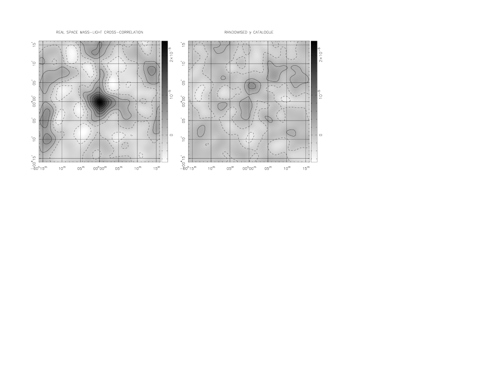
Figure 19: Cross-correlation of light with mass reconstruction and with randomized catalog reconstruction. Left panel shows that actual cross correlation and right panel shows the result of cross correlating the light with a $\kappa$ reconstruction generated from a catalog with randomized (shuffled) shear values.

To see if $M/L$ changes with scale, in figure 20 we show the profile of the luminosity-mass cross-correlation and the luminosity auto-correlation function. These are very similar in shape. We caution that these should in no way be taken to be indicative of the mass-luminosity auto-correlation function in general; the field is small, so the ‘cosmic-variance’ or sampling variance is very large, and the field is also unusual in that it was chosen because it contains a prominent supercluster. What this figure shows though is that aside from a slight enhancement of the luminosity auto-correlation function at very small lag — which might plausibly be due to dynamical segregation — the cross- and auto-correlation functions have very similar shapes indeed. This suggests that on scales $\gtrsim 1^{\prime}$ the early type galaxies trace the mass quite faithfully.

Figure 20: Azimuthally averaged profile of the mass-luminosity cross-correlation function (boxes with error bars) and the luminosity auto-correlation function (circles). In normalizing these we have adopted a mass-to light ratio of $M/L=280h$, somewhat larger than that obtained by simply comparing the correlation strengths at zero lag.

Another way to see if $M/L$ changes with scale is to perform the correlation in Fourier space. The discrete Fourier transform of the $\kappa$ image provides a set of estimates of the actual mass transform which have essentially statistically independent measurement errors. The errors are exactly independent only if the data fully cover the field - here there are some gaps in coverage like the N-W corner which introduce slight correlations between neighboring Fourier coefficients. This slight covariance is properly accounted for by our Monte-Carlo error estimation. The results are shown in figure 21. Here the transform was taken without zero padding. If we use all modes with $k<8$ times the fundamental frequency for our square box (corresponding to wavelengths $\lambda=0.75-6h^{-1}$Mpc) we obtain a correlation which is significant at the the $8.3$-sigma level and we obtain $M/hL=233\pm 28$. If we split the modes into low and high frequency subsets we find $M/hL=280\pm 42$ for $0<k<4$ and $M/hL=176\pm 38$ for $4\leq k<8$ so again, we find a slight, though barely significant, increase in $M/L$ with scale.

Figure 21: Cross-correlation of light with mass reconstruction in Fourier space. Left panel shows that actual cross correlation and right panel shows the result of cross correlating the light with a $\kappa$ reconstruction generated from a catalog with randomized (shuffled) shear values. Box symbols are for modes with $\lambda=1.5-6h^{-1}$Mpc and $+$ symbols are for modes with wavelength $\lambda=0.75-1.5h^{-1}$Mpc.

5 Discussion

The foregoing analysis shows in a number of ways that we have clearly detected the gravitational shear from mass concentrations in this field. All of the major concentrations apparent in the X-ray and optical images are detected in the mass reconstructions, as well as a foreground structure at $z\simeq 0.3$. While the mass reconstructions are somewhat noisy, we have shown by a number of different (though not independent) methods that there is a strong correlation between the observed shear and that predicted assuming early type galaxy light traces the mass, which allow fairly precise estimate of the total mass associated with these galaxies, and we find that the $M/L$ parameter does not vary much with scale.

The dynamical state of the $z\simeq 0.42$ super-cluster is that most of the mass in this region is concentrated into the three clusters. Following ?) we have modeled CL-S as a test particle on a radial orbit around CL-N and CL-E as a test particle on a radial orbit under the combined attraction of CL-N and CL-S. We find generally similar results, but as our masses our somewhat lower than they assumed (by scaling to Coma using the velocity dispersion), our orbital solutions are less tightly bound. We find that CL-S is only marginally bound to CL-N. Equivalently, the mass of CL-N, if spread over a sphere or radius equal to the distance to CL-S, gives a density about equal to that of a critical density Universe at that epoch. We find that CL-E is on an unbound trajectory, though the latter conclusion could possibly be modified if it turns out that CL-N, CL-S have massive neighbors outside of the field we have surveyed. While the clusters are bound and have collapsed, the super-cluster as a whole is still rapidly expanding and may never turn around.

As remarked earlier, the conclusion that early type galaxies trace the mass is rather surprising. The conventional picture of the morphological segregation in superclusters is heavily influenced by the Local Supercluster. There one finds Binggeli et al. (1987) a E-rich core of dimension $\sim 1h^{-1}$Mpc surrounded by a spiral rich ‘halo’ extending to large radii ($\sim 10h^{-1}$Mpc) roughly as $1/r^{2}$ and which dominates the total light. This picture is supported in a statistical sense by the ?) morphology-density relation and also by galaxy correlation studies Loveday et al. (1995). It is commonly assumed either that galaxies in general trace the mass, or, in biased theories and in hot dark matter models, that the mass distribution is even more extended. What we have found is in conflict with either of these pictures; the mass around the clusters in this field is no more extended than the early type galaxies.

Exactly what this implies for the global density parameter $\Omega$ remains somewhat unclear because of the possibility of bias; as with other dynamical estimates of cluster masses one can estimate $M/L$ and then extrapolate to the entire Universe as a simple accounting exercise to obtain the mass density as the product of $M/L$ with the luminosity density measured from redshift surveys, but there is of course no guarantee that the cluster $M/L$’s are really representative. Nonetheless, and with the foregoing caveat, it is of interest to make this extrapolation to obtain $\Omega$ assuming that galaxy formation is unbiased and one can then say what level of bias is implied for other values of $\Omega$.

If we assume that galaxies of all types formed with their usual abundance in this region then we have to ask what has happened to the late types. One possibility is that they are still there and are more broadly distributed than the early types as is the case in other ‘normal’ systems (we know from the spectroscopic studies that they are not in the clusters themselves). Our data do not really support this picture, but we cannot firmly rule it out either. If so, these galaxies have very little mass associated with them, and the total density of the Universe is essentially just the luminosity density in early type galaxies times our $M/L$ and is very small. ?), for example, find a total luminosity density of $\simeq 2\times 10^{8}hL_{\odot}/{\rm Mpc}^{3}$ of which about 20% is due to the early types, and we thereby find $\Omega\simeq 280\times 0.2/1500\simeq 0.04$. The other possibility is that the late type galaxies in this region have, like the early types, fallen into the clusters, but have had their disks extinguished by ram pressure. If there were much mass associated with these galaxies then we should have seen very high mass-to-light ratios for these clusters, but we didn’t, so again this would suggest there is very little mass associated with late types. However, the bulges of the spirals will survive, and would have inflated the cluster luminosity functions at the faint end and the true value of $\Omega$ is then slightly higher.

If galaxy formation was unbiased then, our results suggest a very low value for the density parameter, and, if $h$ is at the lower end of the allowed range, this is mostly or all baryonic. We do not know that early type galaxies are unbiased tracers, but the assumption that they are is at least consistent with the general idea that they formed early (so any statistical bias they may have had a the time of formation may have been washed out) and that they seem to be evolving slowly, and therefore seem to be obeying the continuity equation in an average sense. To avoid this rather radical conclusion one would have to invoke a bias. However, it would seem to be very hard to accommodate these data with say a flat EdS model, since in that case one has a region with net mass density at about or even slightly below the mean, but where the formation of early type galaxies was apparently biased upwards by a factor 20 or so. This seems unreasonable. More modest positive bias cannot be ruled out, and it is also possible that the early type galaxies are ‘anti-biased’; i.e. the abundance of these galaxies per unit mass is lower than average in clusters, in which case the global $\Omega$ is still lower than the above estimate.

We note that our mass determination is blind to any uniform density component, so we cannot rule out the possibility of a contribution to $\Omega$ from very hot dark matter or an ultra-light scalar field, the latter having an effective Jeans length on the order of the geometric mean of the horizon size and the Compton wavelength and which could be very large.

While the density parameter we find seems low as compared to other estimates from e.g. virial analysis (Davis & Peebles (1983); Carlberg et al. (1996)), this is not because our cluster $M/L$ values are much lower, it is because we do not extrapolate to the Universe at large assigning the same $M/L$ to late type galaxies. The interesting new conclusion from our results is that if late types do have the same net $M/L$ as early types — so $\Omega\simeq 0.2-0.3$ — then their formation in the rather large region of space originally occupied by the matter now in the supercluster must have been strongly suppressed and the galaxy formation process must have arranged to create essentially only early type galaxies, and with an abundance several times higher than average to compensate.

Our cluster $M/L$s are considerably lower than that obtained from weak lensing analyses of super-massive clusters like A1689 (e.g. Fischer & Tyson (1997)), and it is interesting to note that the most massive of the three clusters here has a higher $M/L$ than the other two. If these results are indications of a general trend then this would seem to argue against a positive bias for clusters, since the most extreme clusters seem to be less positively biased than more common poorer clusters like those studied here. Equally if $\Omega$ is really $0.2-0.3$ as often assumed then this requires non-monotonicity of bias with both extremely massive clusters and field galaxies being essentially unbiased, but with intermediate mass clusters being positively biased. This seems contrived. Finally, it is also interesting to briefly compare our results with peculiar velocity analyses which provide an alternative probe of the total (dark plus light) mass distribution. Barring some very hot or ultra-light mass component, our low $\Omega$ would seem to be very hard to reconcile with the generally high values found from large-scale ‘bulk-flows’ Dekel (1994). On the other hand, if there is really very little mass outside of clusters, as our data suggest, then this would be compatible with the very cold nature of the Hubble flow in the field (Sandage (1986); Brown & Peebles (1987); Ostriker & Suto (1990)).

6 Acknowledgements

We thank John Tonry, Pat Henry and Harald Ebeling for many helpful conversations and practical aid. GW gratefully acknowledges financial support from the estate of Beatrice Watson Parrent, from Mr. & Mrs. Frank W. Hustace, Jr., and from Victoria Ward, Limited. This work was supported by NASA grant NAG5-7038, NSF grant AST95-00515, NASA grants NAG5-1880 and NAG5-2523, and CNR-ASI grants ASI94-RS-10 and ARS-96-13. H.D. acknowledges support from a research grant provided by the Research Council of Norway, project number 110792/431.

References

- Abell (1958) Abell, G. O. 1958, ApJS, 3, 211
- Bardeen et al. (1986) Bardeen, J., Bond, J., Kaiser, N., & Szalay, A. 1986, ApJ, 304, 15
- Binggeli et al. (1987) Binggeli, B., Tammann, G. A., & Sandage, A. 1987, AJ, 94, 251
- Bond et al. (1996) Bond, J. R., Kofman, L., & Pogosyan, D. 1996, Nature, 380, 603
- Bonnet et al. (1993) Bonnet, H., Fort, B., Kneib, J. P., Mellier, Y., & Soucail, G. 1993, A&A, 280, L7
- Bonnet et al. (1994) Bonnet, H., Mellier, Y., & Fort, B. 1994, ApJ, 427, L83
- Bower & Smail (1997) Bower, R. G., & Smail, I. 1997, MNRAS, 290, 292
- Brainerd et al. (1996) Brainerd, T. G., Blandford, R. D., & Smail, I. 1996, ApJ, 466, 623
- Brown & Peebles (1987) Brown, M. E., & Peebles, P. J. E. 1987, ApJ, 317, 588
- Carlberg et al. (1996) Carlberg, R. G., Yee, H. K. C., Ellingson, E., Abraham, R., Gravel, P., Morris, S., & Pritchet, C. J. 1996, ApJ, 462, 32
- Clowe et al. (1998) Clowe, D., Kaiser, N., Luppino, G., Henry, J. P., & Gioia, I. M. 1998, ApJ, 497, L61, http://xxx.lanl.gov/abs/astro-ph/9805177
- Coleman et al. (1980) Coleman, G. D., Wu, C.-C., & Weedman, D. W. 1980, ApJS, 43, 393
- Cowie et al. (1996) Cowie, L. L., Songaila, A., Hu, E. M., & Cohen, J. 1996, AJ, 112, 839
- Dahle et al. (1994) Dahle, H., Maddox, S. J., & Lilje, P. B. 1994, ApJ, 435, L79
- Davis & Peebles (1983) Davis, M., & Peebles, P. J. E. 1983, ApJ, 267, 465
- Dekel (1994) Dekel, A. 1994, ARA&A, 32, 371
- Dell’Antonio & Tyson (1996) Dell’Antonio, I. P., & Tyson, J. A. 1996, ApJ, 473, L17
- Dickey & Lockman (1990) Dickey, J. M., & Lockman, F. J. 1990, ARA&A, 28, 215
- Dressler (1980) Dressler, A. 1980, ApJ, 236, 351
- Dressler & Gunn (1992) Dressler, A., & Gunn, J. E. 1992, ApJS, 78, 1
- Efstathiou et al. (1988) Efstathiou, G., Ellis, R. S., & Peterson, B. A. 1988, MNRAS, 232, 431
- Ellingson et al. (1997) Ellingson, E., Yee, H. K. C., Abraham, R. G., Morris, S. L., Carlberg, R. G., & Smecker-Hane, T. A. 1997, ApJS, 113, 1
- Fabricant et al. (1994) Fabricant, D. G., Bautz, M. W., & McClintock, J. E. 1994, AJ, 107, 8
- Fahlman et al. (1994) Fahlman, G., Kaiser, N., Squires, G., & Woods, D. 1994, ApJ, 437, 56, http://xxx.lanl.gov/abs/astro-ph/9402017
- Fern’andez-Soto et al. (1998) Fern’andez-Soto, A., Lanzetta, K. M., & Yahil, A. 1998, ApJsubmitted
- Fischer et al. (1997) Fischer, P., Bernstein, G., Rhee, G., & Tyson, J. A. 1997, AJ, 113, 521
- Fischer & Tyson (1997) Fischer, P., & Tyson, J. A. 1997, AJ, 114, 14
- Fort & Mellier (1994) Fort, B., & Mellier, Y. 1994, A&A Rev., 5, 239
- Fort et al. (1996) Fort, B., Mellier, Y., Dantel-Fort, M., Bonnet, H., & Kneib, J. P. 1996, A&A, 310, 705
- Gioia & Luppino (1994) Gioia, I. M., & Luppino, G. A. 1994, ApJS, 94, 583
- Gioia et al. (1990) Gioia, I. M., Maccacaro, T., Schild, R. E., Wolter, A., Stocke, J. T., Morris, S. L., & Henry, J. P. 1990, ApJS, 72, 567
- Giraud (1992) Giraud, E. 1992, A&A, 259, L49
- Greisen & Calabretta (1995) Greisen, E. W., & Calabretta, M. 1995, ASP Conf. Ser. 77: Astronomical Data Analysis Software and Systems IV, 4, 233
- Griffiths et al. (1996) Griffiths, R. E., Casertano, S., Im, M., & Ratnatunga, K. U. 1996, MNRAS, 282, 1159
- Henry (1998) Henry, J. P. 1998, in preparation
- Hudson et al. (1998) Hudson, M. J., Gwyn, S. D. J., Dahle, H., & Kaiser, N. 1998, ApJ, in press, pp, http://xxx.lanl.gov/abs/astro-ph/9711341
- Kaiser (1988) Kaiser, N. 1988, in preparation, lensing methods paper
- Kaiser (1991) Kaiser, N. 1991, ApJ, 358, 1
- Kaiser (1998) Kaiser, N. 1998, ApJ, 498, 26, http://xxx.lanl.gov/abs/astro-ph/9610120
- Kaiser & Squires (1993) Kaiser, N., & Squires, G. 1993, ApJ, 440, 441
- Kaiser et al. (1995) Kaiser, N., Squires, G., & Broadhurst, T. 1995, ApJ, 449, 460, http://xxx.lanl.gov/abs/astro-ph/9411005
- Kaiser et al. (1988) Kaiser, N., Wilson, G., Luppino, G., & Dahle, H. 1988, in preparation, image processing pipeline
- Loveday et al. (1995) Loveday, J., Maddox, S. J., Efstathiou, G., & Peterson, B. A. 1995, ApJ, 442, 457
- Loveday et al. (1992) Loveday, J., Peterson, B. A., Efstathiou, G., & Maddox, S. J. 1992, ApJ, 390, 338
- Luppino & Kaiser (1997) Luppino, G., & Kaiser, N. 1997, ApJ, 475, 20, http://xxx.lanl.gov/abs/astro-ph/9601194
- Luppino et al. (1995) Luppino, G., Metzger, M., Kaiser, N., Clowe, D., Gioia, I., & Miyazaki, S. 1995, in 1995 PASP Conference ‘‘Clusters of Galaxies’’
- Mathez et al. (1992) Mathez, G., Fort, B., Mellier, Y., Picat, J. P., & Soucail, G. 1992, A&A, 256, 343
- Mellier et al. (1994) Mellier, Y., Dantel-Fort, M., Fort, B., & Bonnet, H. 1994, A&A, 289, L15
- Monet (1998) Monet, D. 1998, www
- Mould et al. (1994) Mould, J., Blandford, R., Villumsen, J., Brainerd, T., Smail, I., Small, T., & Kells, W. 1994, MNRAS, 271, 31
- Ostriker & Suto (1990) Ostriker, J. P., & Suto, Y. 1990, ApJ, 348, 378
- Sandage (1986) Sandage, A. 1986, ApJ, 307, 1
- Sarazin (1988) Sarazin, C. L. 1988, in Cambridge ; New York : Cambridge University Press, 1988., 227...
- Sawicki et al. (1997) Sawicki, M. J., Lin, H., & Yee, H. K. C. 1997, AJ, 113, 1
- Schlegel et al. (1998) Schlegel, D. J., Finkbeiner, D. P., & Davis, M. 1998, ApJ, 500, 525
- Schneider (1998) Schneider, P. 1998, ApJ, 498, 43
- Schneider et al. (1998) Schneider, P., Van Waerbeke, L., Mellier, Y., Jain, B., Seitz, S., & Fort, B. 1998, A&A, 333, 767
- Seitz et al. (1996) Seitz, C., Kneib, J. P., Schneider, P., & Seitz, S. 1996, A&A, 314, 707
- Smail & Dickinson (1995) Smail, I., & Dickinson, M. 1995, ApJ, 455, L99
- Smail et al. (1997) Smail, I., Ellis, R. S., Dressler, A., Couch, W. J., Oemler, J., Augustus, Sharples, R. M., & Butcher, H. 1997, ApJ, 479, 70
- Snowden (1998) Snowden, S. L. 1998, ApJS, 117, 233
- Stocke et al. (1991) Stocke, J. T., Morris, S. L., Gioia, I. M., Maccacaro, T., Schild, R., Wolter, A., Fleming, T. A., & Henry, J. P. 1991, ApJS, 76, 813
- Tyson & Fischer (1995) Tyson, J. A., & Fischer, P. 1995, ApJ, 446, L55
- Tyson et al. (1984) Tyson, J. A., Valdes, F., Jarvis, J. F., Mills, A. P., & , J. 1984, ApJ, 281, L59
- Tyson et al. (1990) Tyson, J. A., Wenk, R. A., & Valdes, F. 1990, ApJ, 349, L1
- Valdes et al. (1983) Valdes, F., Jarvis, J. F., & Tyson, J. A. 1983, ApJ, 271, 431