The distribution of nearby stars in phase space mapped by Hipparcos

Abstract

A volume limited and absolute magnitude limited sample of A-F type dwarfs within 125 parsecs of the Sun is searched for inhomogeneities in the density-velocity space, expecting signatures of the cluster evaporation, phase mixing and possible disc heating mechanisms. A 3-D wavelet analysis is used to extract inhomogeneities, both in the density and velocity distributions. Thus, a real picture of the phase space is produced. Not only are some clusters and streams detected, but the fraction of clumped stars can be measured. By estimating individual stellar ages one can relate the streams and clusters to the state of the interstellar medium (ISM) at star formation time and provide a quantitative view of cluster evaporation and stream mixing. As a result, we propose a coherent interpretation of moving groups or so-called superclusters and derive some quantitative evolutionary tracers which we expect to serve in the understanding of the large scale evolution of the galactic disc.
The sample is relatively well mixed in the position space since less than 7 per cent of the stars are proper motion confirmed cluster members. We also detect star evaporation out of the Hyades open cluster.
Only two components of the velocity vectors are provided by Hipparcos measurements. Then, the 3D velocity field is reconstructed from a statistical convergent point method. The wavelet analysis exhibits strong velocity structuring at typical scales of velocity dispersion $\overline{\sigma}_{stream}\sim$ 6.3, 3.8 and 2.4 $km\cdot s^{-1}$. The majority of large scale velocity structures ($\overline{\sigma}_{stream}\sim$ 6.3 $km\cdot s^{-1}$) are Eggen’s superclusters. As illustrated by the Pleiades supercluster these structures are all characterized by a large age range which reflects the overall sample age distribution. These large velocity dispersion structures represent 63$\%$ of the sample. This percentage drops to 46$\%$ if we subtract the velocity background expected by a smooth velocity ellipsoid in each structure. Smaller scales ($\overline{\sigma}_{stream}\sim$ 3.8 and 2.4 $km\cdot s^{-1}$) reveal that superclusters are always substructured by 2 or more streams which generally exhibit a coherent age distribution. At these scales, the contribution of background stars is negligible and percentages of stars in streams are 38$\%$ and 18$\%$ respectively. The detailed analysis of the phase space structures provides a scenario of kinematical evolution in the solar neighbourhood: star formation in the galactic disc occurs in large bursts (possibly subdivided into smaller bursts) separated by quiescent periods. The velocity space is gradually populated by these star formation bursts which preferentially fill the center of the velocity ellipsoid. Stars form in groups reflecting the clumpy structure of the ISM: about 75$\%$ of recently formed stars belong to streams whose internal velocity dispersions do not exceed 4 $km\cdot s^{-1}$. Most of them dissolve rapidly. A fraction of the initial groups are gravitationally bound and form open clusters. Open clusters sustain a longer term streaming with quite similar velocity by an evaporation process due to internal processes or encounters with permanent or transient large mass concentrations. These streams are detected with $\overline{\sigma}_{stream}\sim$ 2.3 and 3.8 $km\cdot s^{-1}$ and have a coherent age content. This process explains the survival of streams up to $10^{9}$ yr. The existence of streams as old as 2 Gyr seems to require other physical mechanisms. The typical scale of so-called Eggen’s superclusters ($\overline{\sigma}_{stream}\sim$ 6.3 $km\cdot s^{-1}$) does not seem to correspond to any physical entity. The picture they form, their frequency and their divisions at smaller scales are well compatible with their creation by chance coincidence of physically homogeneous smaller scale structures ($\overline{\sigma}_{stream}\sim$ 3.8 or 2.4 $km\cdot s^{-1}$).

1 Introduction

1.1 A tentative observation of the stellar gas kinetics

Providing a complete probe of the kinematics of early type stars within a well defined local sphere, Hipparcos data Hip97 (ESA, 1997) offer the first opportunity to get an unbiased look into the stellar kinematics at small scales. In paper I (Crézé et al, (1998)), we used the average density trend and vertical velocity dispersion to map the potential well across the galactic plane. Beyond this 0-order analysis, we now try to get a picture of the kinematic mixture, its inhomogeneities at small scales and their dating. This paper explains the methods used and gives the general results obtained with our sample. Details both in the methodology and the results can always be found in Chereul et al, (1998) (hereafter Paper III). A fourth paper will be dedicated to the physical interpretation of evolutionary aspects.
Wavelet analysis is extensively used to extract deviations from smooth homogeneity, both in density (clustering) and velocity distribution (streaming). A 3-D wavelet analysis tool is first developed and calibrated to recognize physical inhomogeneities among random fluctuations. It is applied separately in the position space (Section 4) and in the velocity space (Section 5). Once significant features are isolated (whether in density or in velocity), feature members can be identified and their behaviour can be traced in the complementary space (velocity or density). Thus, a real picture of the phase space is produced. Not only are some clusters and streams detected, but the fraction of stars involved in clumpiness can be measured. Then, estimated stellar ages help connecting streams and clusters to the state of the ISM at star formation time and providing a quantitative view of cluster melting and stream mixing at work.
Only once this picture has been established on a prior-less basis we come back to previously known observational facts such as clusters and associations, moving groups or so-called superclusters. As a result, we propose a coherent interpretation of this phenomenology and derive some quantitative evolutionary tracers which we expect to serve in the understanding of the large scale evolution of the galactic disc.
A sine qua non condition for this analysis to make sense is the completeness of data within well defined limits. In so far as positions, proper motions, distances, magnitudes and colours are concerned, the Hipparcos mission did care. Things are unfortunately not so simple concerning radial velocities and ages. More than half radial velocities are missing and the situation regarding Strömgren photometry data for age estimation is not much better. So we developed palliative methods which are calibrated and tested on available true data to circumvent the completeness failure. The palliative for radial velocities is based on an original combination of the classical convergent point method with the wavelet analysis, it is presented in Paper III, Section 5.1. The palliative for ages (Section 3) is an empirical relationship between age and an absolute-magnitude/colour index. It has only statistical significance in a very limited range of the HR diagram.

1.2 Review of known facts

While clumpy at the time of star formation, the distribution of stars in phase space gradually evolves towards a state of smoother homogeneity. The precise mechanism of this mixing is not elucidated: there are reports of moving groups (also named superclusters by Eggen) with large velocity dispersions (6-8 $km\cdot s^{-1}$) surviving after many galactic rotations (Eggen 1991, 1992abc) although not obviously bound by internal gravitation. Considering the very short phase mixing time (a few 10⁸ yr, Hénon, (1964)) such streams, exhibiting also large age ranges, cannot be explained by the fact that stars originate in a same cell of the phase space.
The study of these moving groups is extensive. A large part of the recent work deals with their precise identification among early-type (O through F spectral types) main sequence stars (Gomez et al, 1990, Chen et al, 1997, Figueras et al, 1997, and Chereul et al, 1997) which permit both to probe them far from the Sun and to have an individual age estimation using Strömgren photometry (Figueras et al, (1991) and Asiain et al, 1997). Nevertheless, their age content which sometimes spreads over several hundred million years, as noticed in Eggen’s work, is still a puzzle. Two main explanations have been suggested. On one hand, a supercluster is formed from several star formation bursts occurring at different times in a common molecular cloud (Weidemann et al, 1992) which experiences perturbations such as large scale spiral shocks (Comerón et al, 1997). These bursts can be gravitationally bound and maintain streams by cluster evaporation process during their lifetime. Dynamics of star clusters and giant molecular clouds (hereafter GMC) in the galactic disc are different. Thus, different star formation episodes in a same GMC separated by several galactic rotation periods will hardly result in giving a supercluster velocity structure. On other hand, asupercluster is a chance superposition of several cluster evaporations or remnants (and also phase mixing process of unbound recent groups) in a same cell of the phase space. Then, a supercluster-like velocity structure do not need any physical process to be maintained. At a given time in the solar neighbourhood, the juxtaposition at random of several cluster remnants creates over densities in the velocity field which mimics the existence of a physical entity with large velocity dispersion.

1.3 Hipparcos sample

Hipparcos data Hip97 (ESA, 1997), providing accurate distances and proper motions for complete volume limited samples of nearby stars, offer the first opportunity to look at the phase mixing process and the disc heating mechanisms in action. Such signatures are searched for with a sample that provides all the stars with same physical properties within a well defined volume. The sample was pre-selected inside the Hipparcos Input Catalogue (ESA, (1992)) among the “Survey stars”. The limiting magnitude is $m_{v}\leq 7.9+1.1\cdot\sin\mid b\mid$ for spectral types earlier than G5 (Turon & Crifo, (1986)). Spectral types from A0 to G0 with luminosity classes V and VI were kept. Within this pre-selection the final choice was based on Hipparcos magnitude ($m_{v}\leq 8.0$), colours ($-0.1\leq B-V\leq 0.6$), and parallaxes ($\pi\geq 8mas$). The sample studied (see sample named h125 in Paper I, Crézé et al, (1998)) is a slice in absolute magnitude of this selection containing 2977 A-F type dwarf stars with absolute magnitudes brighter than 2.5. It is complete within 125 pc from the Sun.

1.4 Where to find…

The wavelet analysis procedure is described and discussed in Section 2. Age determination methods follow in Section 3. Main results of the density analysis in position space (clustering) are given in Section 4. The analysis of the velocity space (streaming) is given in Section 5. A critical review of uncompleteness and other systematic effects can be found in Paper III, Sections 5.1 and 5.2. Section 5.5 presents our understanding of the supercluster concept based on all the results detailed in Paper III. Conclusions in Section 6 present a simple scenario which organizes the main results of this paper to explain observed phase space structures in the solar neighbourhood.

2 Density-velocity analysis using wavelet transform

An objective method should first be adopted to identify structures and determine their characteristic scales and amplitudes. The wavelet transform does provide such an accurate local description of signal characteristics by projecting it onto a basis of compactly supported functions (Daubechies, (1991)). The basis of wavelet functions is obtained by dilatation and translation of a unique, oscillating and zero integral function: the mother wavelet. The wavelet representation gives signal characteristics in terms of location both in position and scale simultaneously.

2.1 The wavelet transform

The wavelet transform by $\Psi(x)$ of a real one-dimensional signal $F(x)$ is defined as the scalar product:

$$W_{s}(i)=\frac{1}{\sqrt{s}}\int^{+\infty}_{-\infty}F(x)\cdot\Psi^{\ast}(\frac{x-i}{s})dx\\$$ (1)

where $s$ is the scale and $i$ the position of the analysis. Shape and properties of the so-called mother wavelet $\Psi(x)$ are similar to a Mexican Hat and ensure a quasi-isotropic wavelet transform of the signal. It is constructed from a $B_{3}$ spline function $\Phi(x)$ which is compact and regular up to the second order derivative:

$$\Phi(x)=(\mid x-2\mid^{3}-4\mid x-1\mid^{3}+6\mid x\mid^{3}$$

$$\hskip 28.45274pt-4\mid x+1\mid^{3}+\mid x+2\mid^{3})/12$$ (2)

leading to:

$$\Psi(x)=\Phi(x)-\frac{1}{2}\Phi(\frac{x}{2})\\$$ (3)

The 3-D scaling function $\Phi(x,y,z)$ used to analyze the observed $F(x,y,z)$ distribution is a separable function

$$\Phi(x,y,z)=\Phi(x)\cdot\Phi(y)\cdot\Phi(z)\\$$ (4)

Among several possible implementations of the wavelet analysis, the “à trou” algorithm, previously used for the analysis of large scale distribution of galaxies (Lega et al, 1996, Bijaoui et al, 1996) has been selected. The reasons for this choice and the principles of the method are given in the following Section.

2.2 The “à trou” algorithm

Two main lines of algorithms have been used in order to implement the wavelet analysis concept. The pyramidal approach (Mallat, (1989)), used by Meneveau (1991) for turbulence analysis, with orthogonal wavelet basis addresses orthogonality problems in a rigorous way but it fails providing convenient tools to localize structures. On the contrary, the “à trou” algorithm associated with non orthogonal wavelet basis, giving an identical sampling at each scale (same number of wavelet coefficients at each scale), is appropriate for such practical purpose. For a detailed description of the “à trou” algorithm the reader is referred to Holschneider et al (1989), Starck (1993), Bijaoui et al (1996) and details are also provided in Paper III.
The 3-D distribution $F(x,y,z)$ is binned in a 128 pixel edge cube which is wavelet analyzed on five dyadic scales. The analyzing function is dilated so that the distance between two bins increases by a factor 2 from scale $s-1$ to scale $s$. So it is a suitable framework in which local over-densities of unknown scales and low amplitude can be pointed at. The wavelet coefficient value depends on the gradient of the signal $F(x,y,z)$ in the neighbourhood of point $(i,j,k)$ considered at a given scale $s$: the absolute value of the coefficient increases all the more since the signal varies on this scale. For a positive or null signal like the observed distributions (star counts in the solar neighbourhood), over-density structures mainly lead to strong positive values of wavelet coefficients while under-densities cause strong negative coefficients.

2.3 Thresholding and segmentation

Once the wavelet decomposition of the real signal is obtained, significant wavelet coefficient structures are separated from those generated by random fluctuations of a uniform background. A thresholding is applied at each scale in the space of wavelet coefficients. Thresholds are set at each scale and each position by estimating the noise level generated at the same scale by a uniform random signal built with the same gross-characteristics as the observed one at the position considered. Then a segmentation procedure returns pixel by pixel the characteristic extent of structures in each dimension. The thresholding and segmentation procedures are sketched out in Paper III.

Since we are aiming at an estimation of the total fraction of stars actually involved in physical structures, one has to care for the casual presence of background stars at the position (or velocity) of structures. Cluster membership is classically tested by the coincidence of tangential velocities (Section 4.1). This is not possible for stream membership. In this last case, only the fraction of non-members can be evaluated (Paper III, Section 5.2). Eventually the age distribution of members is discussed in the light of various possible scenarii.

3 Individual age determination

3.1 Introduction

In order to bridge the observed phenomenology with the galaxy evolution, it is essential that structures in the phase space be dated. Once structure members have been duly identified they should be given an age. Strömgren photometry is available for some 1608 stars out of a total sample of 2977. When Strömgren photometry is available, ages are estimated in a now classical way (Section 3.2). There is however a strong suspicion that the age distribution of stars observed in Strömgren photometry is biased. At least, even though observers are not likely to have selected their targets on a prior age indicator, they are likely to have favoured stars in clusters and streams, which is highly damageable for the present investigation. In order to correct at least statistically the suspected resulting bias, we propose an empirical palliative age estimation method based on the Hipparcos absolute magnitude and colour. This method is fully described in Paper III.

3.2 Ages from Strömgren photometry

We find 1608 stars with published Strömgren photometry (Hauck & Mermilliod, 1990) in our sample. For this sub-sample, the effective temperature $T_{eff}$, the surface gravity $\log g$ and their errors, the metallicity [Fe/H] are derived from the photometric indices $(b-y)$, $m1$, $c1$, $H_{\beta}$, the visual magnitude $m_{v}$ and the rotational velocities $v\cdot\sin i$ (if published in Uesugi & Fukuda, (1981)) using a program developed by E. Masana (Figueras et al, (1991), Masana, (1994), Jordi et al, (1997)). Based on the above three physical parameters and a model of stellar evolution taking into account overshooting effects and mass loss (Schaller et al, 1992), ages and masses are inferred with the code developed by Asiain (Asiain et al, 1997). By means of the stellar metallicity, this algorithm interpolates the set of stellar evolutionary models to work at the appropriate metallicity. Ages and masses determination were possible for only 1077 stars (a third of the sample) due to the failure of the method to get reliable metallicities for spectral types between A0 and A3.

The mean error on age determination is 30 $\%$ ($\sim$0.2 in logarithmic scale) for the bulk of the stars (Figure 1) and rarely exceed 60 $\%$ ($\sim$0.3 in logarithmic scale). Only the youngest stars, between 10⁷ and 10⁸ years, have errors above 100 $\%$ ($\sim$0.5 in logarithmic scale). Nevertheless, this precision is sufficient to unambiguously attach them to the youngest age group.

Figure 1: Strömgren age determinations and their errors for 1077 stars.

The distribution of Strömgren ages (Figure 2) for these 1077 stars ranges from 10 Myr to 3 Gyr with a peak around 650 Myr ($\log$(age) = 8.8).

3.3 Palliative ages from $(M_{v},(B-V))$

On a first step, we use existing ages to draw a plot of ages versus (Mv, (B-V)). A primary age parameter is assigned as the mean age associated to a given range of (Mv, (B-V)). Then Strömgren age data are used a second time to assign a probability distribution of palliative ages as a function of the primary age parameter (See details in Paper III).

Figure 2: Strömgren age distribution obtained with 1077 stars (full line) and palliative age distribution for the same sub-sample (dotted line).

Figure 3: Strömgren age distribution obtained with 1077 stars (full line) and palliative age distribution for the remainder, i.e stars without Strömgren photometry (dotted line).

This process produces a palliative age distribution which is free from possible biases affecting the sub-sample of stars with Strömgren photometry for stars with B-V $\geq$ 0.08.
The palliative age distribution of stars with Strömgren photometry is presented on Figure 2. The small deviations from the distribution of original Strömgren ages are due to finite bin steps used in the discretisation process. The palliative age distribution of the sub-sample without Strömgren photometry (Figure 3) shows a great difference for very young ages with respect to the Strömgren age distribution. The great peak at $10^{7}$yr means that more than 400 stars are clearly younger than 2-3 $10^{8}$ yr (see explanations in Paper III) and compose a separate population from the rest of the sample.
These palliative ages have only statistical significance. Hence, they sometimes produce artifacts or young ghost peaks in some stream age distributions. Such dummy young peaks will always appear as the weak counterpart of a heavy peak around $log(age)=8.7$. Nevertheless palliative ages permit to shed light on the age content of the phase space structures when Strömgren data are sparse.

4 Clustering

4.1 Searching for clusters

(X,Y,Z) distributions range from -125 pc to +125 pc and are binned in a Sun centered orthonormal frame, X-axis towards the galactic center, Y-axis in the rotation direction and Z-axis towards the north galactic pole. The discrete wavelet analysis is performed on five scales: 9.7, 13.6, 21.5, 37.1 and 68.3 pc. These values correspond to the size of the dilated filter at each scale.
Over-densities are identified at each scale (Figure 4) by the segmentation procedure and the stars belonging to each volume are collected. Due to the over-sampling of the signal by the “à trou” algorithm, some structures are detected on several scales. A cross-correlation has been done between all scales to keep the structure at the largest scale provided that there is no sub-structure at a lower scale (higher resolution). An iterative 2.5 sigma clipping procedure on tangential velocity distributions for each group remove field stars and select structures with coherent kinematics.
The same work has been performed to search for under-densities (signed by negative wavelet coefficients). No convincing evidence of the presence of void has been found. In the following we only pay attention to the detection of over-densities.

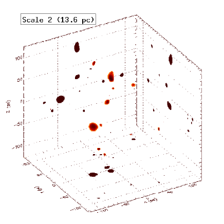
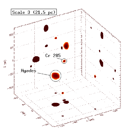
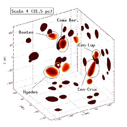
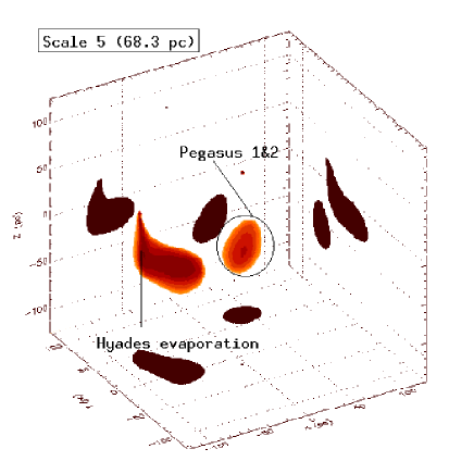
Figure 4: Significant over-densities in wavelet coefficient spaces for space distributions (grey clumps) and their projections on the three main planes (black clumps): (X,Y) plane (bottom) - (Y,Z) plane (right) - (X,Z) plane (background). Some cluster identifications are given. Scale 2, 3, 4 and 5.

4.2 Main results

The space distribution is essentially smooth at all scales. The volumes selected by the segmentation procedure contain 10 per cent of the stars. After the 2.5 sigma clipping procedure on the tangential velocities, only 7 per cent are still in clusters or groups. Most of them are well known: Hyades, Coma Berenices, Ursa Major open clusters (hereafter OCl) and the Scorpio-Centaurus association. Otherwise, three new groups, probably loose clusters, are detected: Bootes and Pegasus 1 and 2. Paper III provides a detailed review of all these cluster characteristics. Here, we just focus on a newly discovered feature concerning the Hyades OCl: its evaporation track.

The Hyades open cluster’s tail is clearly visible at scale 5 on Figure 4. After selection on tangential velocities, 39 stars of the over-density tail are found to have similar motions (Figure 5). The tangential velocity component along the $l$ axis is nearly the same as the Hyades OCl’s one (20.8 $km\cdot s^{-1}$ vs. 19.4 $km\cdot s^{-1}$ respectively) but differs along the $b$ axis (-2.6 $km\cdot s^{-1}$ vs. 14.2 $km\cdot s^{-1}$ respectively). The extremely peaked age distribution at $5-6.3\cdot 10^{8}$ yr shows that stars are slightly younger on average than the Hyades’ ones ($6.3-8\cdot 10^{8}$ yr). Both age determinations are in agreement with recent age determination by Perryman et al (1998) who give $6.25\pm 0.5\cdot 10^{8}$ yr.

Figure 5: The Hyades open cluster’s tail after selection on tangential velocities (top) and its age distribution (middle), Hyades OCl members age distribution (bottom).

Nevertheless, the density distribution along the tail are a spectacular confirmation of the theoretical predictions proposed by Weidemann et al (1992) concerning the distributions of evaporated stars from the Hyades OCl. These authors expect stars evaporated from the Hyades to be distributed in a needlelike ellipsoid centred on the cluster center and with longest axis pointing towards $(l=97.7^{o},b=+1.7^{o})$. The space distribution of the 39 stars exhibit an obvious major axis, with respect to the Hyades OCl, pointing towards $(l=94.0^{o},b=+7.0^{o})$ but are only distributed further forward in the direction of Galactic rotation. This feature can be produced by escaping stars orbiting closer to the Galactic center than the cluster members (Weidemann et al, 1992). These stars have a smaller guiding radius implying a shorter rotation period. The authors speculate for this type of escaping stars, the existence of a phase advance in the vertical oscillation which could agree with the difference observed in the $T_{b}$ components. Moreover, we observe these stars higher in the plane as it is expected because the open cluster is on the upswing.
It is striking to notice that stars as massive as 1.8$M_{\odot}$ (which is the typical mass in our sample) are also evaporating from the cluster. Whatever the cause of the “evaporation” process, slow random change of star binding energies due to a large number of weak encounters (Chandrasekhar, 1942) or sudden energy increase by few close encounters (Hénon, 1960) inside the cluster, it produces a mass segregation among still clustered stars. Indeed, low mass stars are preferentially evaporated and massive stars are retained as shown by means of numerical simulations in Aarseth (1973) and Terlevich (1987) and as reported in Reid (1992) who find a steeper density gradient among the brighter Hyades stars. The asymmetry in the density distribution of the escaping stars could have two main explanations. We cannot rule out a non detection by the wavelet analysis of a symmetric tail provided that its size is larger than the coarser scale of analysis. But if it were not the case, it might sign an encounter between the Hyades OCl and a massive object on the Galactic center side of the cluster. This hypothesis was previously investigated by Perryman et al (1998) who find it highly improbable because of the velocity with respect to the LSR (30 $km\cdot s^{-1}$) and the mass ($\sim 10^{6}M_{\odot}$) needed for such an object. A more detailed analysis should be done to conclude on the origin of this tail.

5 Streaming

5.1 Mean velocity field

Global characteristics of the triaxial velocity ellipsoid are obtained from a sub-sample of 1362 stars which have observed and published radial velocities (ESA, (1992)). The centroid and the velocity dispersions in the orthonormal frame centred on the Sun’s velocity with U-axis towards the galactic center, V-axis towards the rotation direction and W-axis towards the north galactic pole, are the following:

• $\overline{U}_{sample}$ = -10.83 $km\cdot s^{-1}$ and $\sigma_{U}$= 20.26 $km\cdot s^{-1}$

• $\overline{V}_{sample}$ = -11.17 $km\cdot s^{-1}$ and $\sigma_{V}$= 12.60 $km\cdot s^{-1}$

• $\overline{W}_{sample}$ = -6.94 $km\cdot s^{-1}$ and $\sigma_{W}$= 8.67 $km\cdot s^{-1}$
  

The sub-sample with observed radial velocities is incomplete and contains biases since the stars are not observed at random. To keep the benefits of the sample completeness, a statistical convergent point method is developed to analyze all the stars (see Paper III, Section 5.1).

5.2 Wavelet analysis of the velocity field

In a recent paper Dehnen (1998) criticizes this methodology which could be less rigorous than maximizing the log-likelihood of a velocity distribution model. The author argues that direct determination of velocity dispersions based on a convergent point method produces overestimation and may create spurious structures on small scales by noise amplification. Both risks are clearly ruled out by the calibration process described above :

1. the thresholding is calibrated on numerical experiments so as to exclude spurious structure detection at any meaningful level (see Paper III, Section 2.2).

2. the fraction of spurious members in real groups created by the convergent point method is estimated from the available subset of true 3D velocities based on observed radial velocity data (see Paper III, Section 5.2.1).

3. estimated group velocity dispersions are derived from radial velocity subset as well, excluding convergent point reconstructed data.

The confusion in Dehnen’s comment is probably related to another misunderstanding. In a footnote dedicated to a preliminary version of our work, this author explicitly suggests that the convergent point method “which stems for the times when more rigorous treatment was impractical on technical ground” was adopted by plain anachronism or ignorance of “more rigorous treatment”. Actually, the choice was guided by the requirements of the wavelet analysis which gives access to a fine perception of 3D structures. Dehnen’s analysis fits more rigorously a velocity field model with an initial coarse resolution of 2-3 $km\cdot s^{-1}$ depending on the velocity component considered while our bin step is 0.8 $km\cdot s^{-1}$. As a result we get (calibrated) significant signal one scale below the finest resolution of Dehnen’s work. Moreover, the significance threshold of velocity field features obtained by Dehnen is somewhat arbitrary: features are relevant if they appear in more than one of the studied sub-samples.
Velocities of open cluster stars are poorly reconstructed by this method because their members are spatially close. For such stars, even a small internal velocity dispersion results a poor determination of the convergent point. For this reason, we have removed stars belonging to the 6 main identified space concentrations (Hyades OCl, Coma Berenices OCl, Ursa Major OCl and Bootes 1, Pegasus 1, Pegasus 2 groups) found in the previous spatial analysis. Eventually, the reconstruction of the velocity field is performed with 2910 stars.

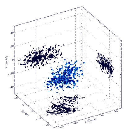
Figure 6: Isosurfaces (grey clumps) in wavelet space after thresholding for velocity distributions - Projections (black clumps) on (U,V) plane (bottom), (V,W) plane (right) and (U,W) plane (background) - Scale 1 (3.2 $km\cdot s^{-1}$).

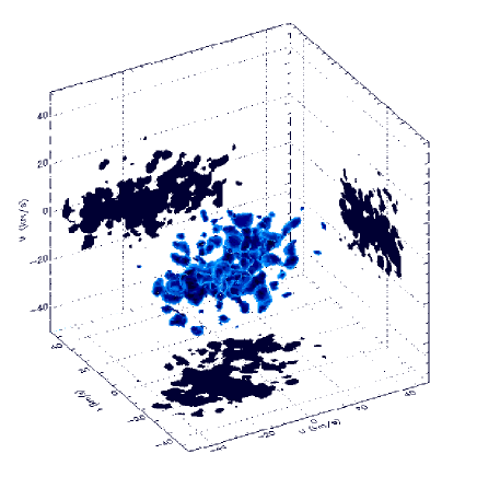
Figure 7: Same as Figure 6 for scale 2 (5.5 $km\cdot s^{-1}$).

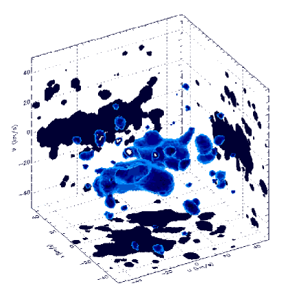
Figure 8: Same as Figure 6 for scale 3 (8.6 $km\cdot s^{-1}$).

Reconstructed (U,V,W) distributions are given in an orthonormal frame centred in the Sun velocity (see Section 5.1) in the range [-50,50] $km\cdot s^{-1}$ on each component. The wavelet analysis is performed on five scales: 3.2, 5.5, 8.6, 14.9 and 27.3 $km\cdot s^{-1}$. In the following, the analysis focuses on the first three scales revealing the stream-like structures (see Figures 6, 7 and 8), larger ones reach the typical size of the velocity ellipsoid. Once the segmentation procedure is achieved, stars belonging to velocity clumps are identify. Structures found in this reconstructed velocity field are contaminated by spurious members created by the method. This contamination is evaluated from the sub-sample with observed $V_{R}$ by a procedure described in Paper III, Section 5.2.1 (hereafter procedure 5.2.1). The proportion of field stars is also evaluated in Paper III, Section 5.2.2 (hereafter procedure 5.2.2).

5.3 Stream phenomenology

The A-F type star 3D velocity field turns out highly structured at the first three scales. In a previous analysis Chereul et al, (1997), it has been found that structures are mainly revealed in the (U,V) plane rather than in the (U,W) plane. This is, probably, the signature of a faster phase mixing process along the vertical axis.
In Paper III, Tables 2, 3 and 4 provide mean velocities, velocity dispersions and numbers of stars remaining after correction procedures 5.2.1 and 5.2.2 for streams at respectively scale 3, 2 and 1. Here, Table 1 summarizes characteristics of the streaming organization. For each scale, Table 1 gives the number of detected velocity groups after wavelet analysis, the number of confirmed streams remaining after elimination of spurious members (procedure 5.2.1) and the fraction of confirmed stars in streams after corrections 5.2.1 and 5.2.2. The number of confirmed streams gives a lower estimation of the real number of streams since sometimes the selection of real members is performed on very few radial velocity data with respect to the potential members. We can notice that the fraction of stars involved in streams at scale 2 ($\sim$ 38 $\%$) is roughly the same as the fraction involved in larger structures at scale 3 ($\sim$46$\%$) when field stars are removed. It already gives a strong indication that large structures at scale 3 could be mainly composed by clustering of streams with smaller velocity dispersions from scale 2.
The wavelet scales can be calibrated a posteriori in terms of stream velocity dispersions. The distribution of mean velocity dispersions ($\overline{\sigma}_{stream}=(\frac{1}{3}\cdot(\sigma_{u}^{2}+\sigma_{v}^{2}+\sigma_{w}^{2}))^{\frac{1}{2}}$) for the streams at a given scale yields a better indicator of the characteristic scale than the filter size (Figure 9). The typical velocity dispersions of detected streams at scales 1, 2 and 3 are respectively 2.4, 3.8 and 6.3 $km\cdot s^{-1}$.
Streams appearing at scale 3 ($\overline{\sigma}_{stream}\sim$ 6.3 $km\cdot s^{-1}$) correspond to the so-called Eggen superclusters. At smaller scales ($\overline{\sigma}_{stream}\sim$ 3.8 and 2.4 $km\cdot s^{-1}$) superclusters split into distinct streams of smaller velocity dispersions.

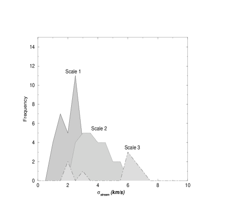
Figure 9: Distribution of stream mean velocity dispersions per scale.

Table 1: Number of streams detected per scale by the wavelet analysis and the percentage of stars involved in streams after cleaning up spurious members and field stars.

Scale	1	2	3
Filter size ($km\cdot s^{-1}$)	3.2	5.5	8.6
$\overline{\sigma}_{stream}$ ($km\cdot s^{-1}$)	2.4	3.8	6.3
Detected velocity groups
after wavelet analysis	63	46	24
Confirmed streams after elimination
of spurious members (Procedure 5.2.1)	38	26	9
$\%$ of stream stars after elimination
of spurious members (Procedure 5.2.1)	17.9$\%$	38.3$\%$	63.0$\%$
$\%$ of stream stars after elimination
of background (Procedure 5.2.1 and 5.2.2)	17.9$\%$	38.3$\%$	46.4$\%$

The age distribution inside each stream is analyzed. The analysis is performed on three different data sets:

• the whole sample (ages are either Strömgren or palliative),

• the sample restricted to stars with Strömgren photometry data (without selection on radial velocity),

• the sample restricted to stars with observed (as opposed to reconstructed) radial velocity data (ages are either Strömgren or palliative).

The selection on photometric ages gives a more accurate description of the stream age content while the last sample permits to obtain a reliable kinematic description since stream members are selected through procedure 5.2.1. All mean velocities and velocity dispersions of the streams are calculated with the radial velocity data set. Combining results from these selected data sets generally brings unambiguous conclusions.
Results obtained for all the streams found on these 3 scales are fully repertoried in Paper III. Here, we focus on the results for the Pleiades supercluster (hereafter Pleiades SCl). This example illustrates very well the advance realized in the understanding of supercluster inner structure.

5.4 Inner structure of the Pleiades supercluster

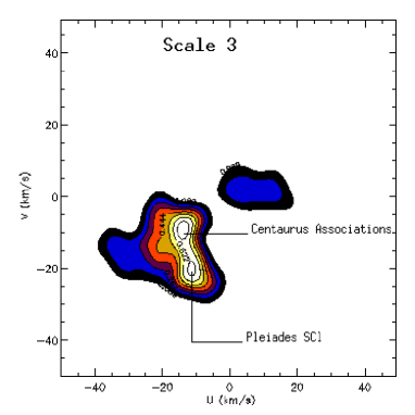
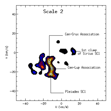
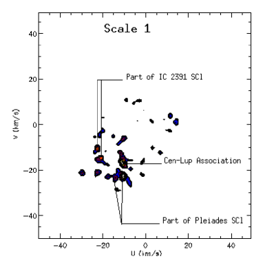
Figure 10: Pleiades SCl. Thresholded wavelet coefficient isocontours at W=-6.2 $km\cdot s^{-1}$ of the velocity field at scale 3 (top), scale 2 (middle) and scale 1 (bottom). Scale 2 shows the dichotomy between Cen-Crux and Cen-Lup associations (streams 2-26 and 2-12 in Paper III, Table 3) embedded in the same clump at scale 3. Scale 1 exhibits clearly the sub-structuring of the Pleiades SCl (streams 1-6 and 1-7 in Paper III, Table 4).

Figure 11: Pleiades SCl. Age distributions of the Pleiades SCl (stream 3-8 in Paper III, Table 2) at scale 3 (top) and scale 2 (stream 2-5 in Paper III, Table 3) (bottom) .

Figure 12: Pleiades SCl. Age distributions of the two sub-streams: stream 1-6 and 1-7 (in Paper III, Table 4) discovered in the Pleiades SCl at scale 1. The oldest population is mainly present in the stream 1-6 (top) while the youngest one composes stream 1-7 (bottom).

The Pleiades supercluster (stream 3-8 in Paper III, Table 2) is detected at scale 3 (see Figure 10 for velocity distributions, Figures 11, 12 for age distributions and Figures 13 for space distributions) and the set of stars selected on their observed radial component gives a mean velocity (U,V,W)=(-14.4,-20.1,-6.2) $km\cdot s^{-1}$ and velocity dispersions ($\sigma_{U},\sigma_{V},\sigma_{W}$)=(8.4,5.9,6.3) $km\cdot s^{-1}$. The age distribution (Figure 11) covers the whole sample age range. The interval is larger than the one mentioned by Eggen (1992a): 6$\cdot 10^{6}$ to 6$\cdot 10^{8}$ yr. Pure Strömgren age distribution, peaks between $6\cdot 10^{8}$ and $10^{9}$ yr. The $V_{R}$ selected set with palliative ages, shows clearly the preponderance of a very young population: a peak at $10^{7}$ yr. A second peak at $6\cdot 10^{8}$ yr is also present. Part of this peak can be due to the statistical age assignation of very young stars as well as to a real stream. But this scale (scale 3) is still too coarse to improve previous analysis.
Scale 2 reveals unambiguously two groups (Figure 11) of mean ages $10^{7}$ and $10^{9}$ yr in stream 2-5 (Paper III, Table 3). The $6\cdot 10^{8}$ year old group is no more present among Strömgren age distribution and the reminiscence found in the palliative age distribution is clearly due to intrinsically very young stars. At this scale, the stream is localized at (U,V,W)=(-12.0,-21.6,-5.3) $km\cdot s^{-1}$ with velocity dispersions ($\sigma_{U},\sigma_{V},\sigma_{W}$)=(5.3,4.7,5.9) $km\cdot s^{-1}$.
At the highest resolution (scale 1) the main velocity clump splits into two components. The first one, at (U,V,W)=(-13.1,-21.9,-7.1) $km\cdot s^{-1}$ with ($\sigma_{U},\sigma_{V},\sigma_{W}$)=(3.1,3.3,2.5) $km\cdot s^{-1}$ (stream 1-6 in Table 4, Paper III) contains almost all the oldest stars ($10^{9}$ yr). The second component at (U,V,W)=(-11.1,-21.9,-5.9) $km\cdot s^{-1}$ with ($\sigma_{U},\sigma_{V},\sigma_{W}$)=(1.7,3.0,1.9) $km\cdot s^{-1}$ (stream 1-7 in Paper III, Table 4) is almost exclusively composed of the youngest population (Figure 12). Moreover, the youngest component has significantly smaller velocity dispersions and its space distribution is more clumpy (Figure 14).
The interpretation comes out quite naturally. The Pleiades SCl is a chance superposition of two main streams originating from two different star formation epochs. One very young stream is a few $10^{7}$ year old and is related with the Pleiades open cluster. The relative large velocity difference with the Pleiades OCl ($\sim$ 8 $km\cdot s^{-1}$) and the space concentration (Figure 14) suggest that these stars were formed from the same interstellar cloud complex and at the same time as the Pleiades OCl, yet separately. The second stream is much older (roughly $10^{9}$ yr) and is probably related to an old cluster loosely bound by internal gravitation which is finishing to dissolve now. The probability to find such a coincidence in the velocity volume covered by the Eggen’s supercluster is quite high (see Section 5.5).

Figure 13: Space distribution of Pleiades SCl obtained from the $V_{R}$ selected sub-sample at scale 3 (stream 3-8 in Paper III, Table 3).

Figure 14: Space distribution of the 2 sub-streams of Pleiades SCl from the V_R selected sub-sample at scale 1: stream 1-6 (top) and stream 1-7 (bottom) in Paper III, Table 4.

5.5 How about Eggen’s superclusters

The review of age and space distributions of the largest velocity structures detailed in paper III puts some classification in the understanding of the so-called superclusters. As it is shown in Section 5.4 for the Pleiades SCl, it is clear that most superclusters, when looked at sufficient resolutions (small scales), split into sub-components covering much restricted age ranges. The question then arises whether superclusters are real significant structures involving stars born at different epochs but tied to the same cell of the phase space by any binding mechanism or are they only chance coincidences between streams at smaller scales, each essentially coeval. In the first case, a complex scenario such as the one proposed by Weidemann et al (1992) might be necessary. In such a scenario, cluster stars are formed at different epochs out of a single molecular cloud and remain gravitationally bound to the cloud. A process which looks hard to maintain over long periods.
It is easy to evaluate the probability that superclusters are formed by chance coincidence of smaller velocity dispersion streams. In Paper III, Section 5.2.2 we computed the fraction of a smooth gaussian 3D distribution embedded in the velocity volume covered by superclusters to estimate the fraction of field stars. This fraction was found to be 0.192 for the 6 identified superclusters. That is an average of 0.032 per supercluster. Under the assumption that the 38 streams appearing at scale 1 with $\overline{\sigma}_{stream}\sim$2.4 $km\cdot s^{-1}$ (see Table 1 and Paper III, Table 4) correspond roughly to 38 real independent causes, most originating at different epochs and different places, the average number of such low dispersion streams expected to occur in a typical supercluster velocity volume is 38$\cdot$0.032=1.216. In Table 2 we give the poissonian probability to get 0, 1, 2… coincidences in any supercluster velocity volume, and the number of superclusters built out of 1, 2,… elementary streams that one would expect to get by chance in the explored velocity volume. The total velocity volume contains 1/0.032=31.2 typical supercluster volumes. These average numbers should be compared with the observed statistics of supercluster richness in elementary streams. Clearly enough no meaning full test at any reasonable significance level can be built to reject the null hypothesis that superclusters have no physical reality.

Table 2: Observed number of superclusters including n or more elementary streams, compared with what would be expected if 38 independent elementary streams were distributed randomly in the whole velocity volume.

n	Probability	Probability	Expected number	Observed number
			of superclusters	of superclusters
	k=n	k$\geq$n	k$\geq$n	k$\geq$n
0	0.296	1
1	0.360	0.704	22.0	26
2	0.219	0.343	10.7	6
3	0.089	0.124	3.9	3
4	0.027	0.035	1.1	1
5	0.007	0.008	0.3	1
6	0.001	0.002	0.1	0

So superclusters most likely result from the chance coincidence in a large cell of the velocity space of several small streams, and the physical interpretation has to be searched for only at the smaller scale. Almost all the phenomena observed here can be explained by a single scenario resulting from two dominant mechanisms: phase mixing and cluster evaporation or disruption. At formation most stars form in clump of the ISM generating short lived streams which dissolve essentially over mixing time scales ($\sim$10⁸ yr): it is probably the case of the Centaurus associations and the very young component of the Pleiades SCl. Only streams massive enough to create some self gravitationally bound systems (more or less loose clusters) survive and create, as they dissolve, moderately old streams with age between 5$\cdot 10^{8}$ and $10^{9}$ yr (see streams in Hyades SCl, Sirius SCl and New SCl in Paper III). In some cases those moderately old streams can be explicitly connected to the cluster they are escaping from (Ursa Major OCl for the old component of Sirius SCl and possibly Coma Berenices OCl for the New SCl 6$\cdot 10^{8}$ year old component). However, there are a few much older groups unrelated to heavy superclusters (streams 3-9, 3-11 and 3-14 in Paper III, Table 2). In those rare cases, all connected to highly eccentric orbits, a completely different mechanism should be advocated which might be trapping on resonant orbits generated by the potential of the bar (Dehnen, 1998).

6 Conclusions

A systematic multi-scale analysis of both the space and velocity distributions of a thin disc young star sample has been performed.
The sample is well mixed in position space since no more than 7$\%$ of the stars are in concentrated clumps with coherent tangential velocities. In this paper we focus on the detection of the evaporation of relatively massive stars (1.8 M$\odot$) out of the Hyades open cluster. The mapping we realized show an asymmetric pattern further forward the Hyades OCl orbit. This could be the signature of a violent encounter on one side of the open cluster with a massive molecular cloud. Such a picture is in agreement with the origin of streams from open cluster evaporation or disruption.
The 3D velocity field reconstructed from a statistical convergent point method exhibits a strong structuring at typical scales of $\overline{\sigma}_{stream}\sim$ 6.3, 3.8 and 2.4 $km\cdot s^{-1}$. At large scale (scale 3) the majority of structures are identified with Eggen’s superclusters. These large scale velocity structures are all characterized by a large age range which reflects the overall sample age distribution. Moreover, few old streams of $\sim$ 2 Gyr are also extracted at this scale with high U components towards the Galactic center (see Paper III). Taking into account the fraction of spurious members, evaluated with an observed radial velocity data set, into all these large velocity dispersion structures we show that they represent 63$\%$ of the sample. This percentage drops to 46$\%$ if we remove the velocity background created by a smooth velocity ellipsoid in each structure. Smaller scales ($\overline{\sigma}_{stream}\sim$ 3.8 and 2.4 $km\cdot s^{-1}$) reveal that superclusters are always substructured by 2 or more streams which generally exhibits a coherent age distribution. The older the stream, the more difficult the age segregation between close velocity clumps inside the supercluster velocity volume. At scale 2 and 1, background stars are negligible and percentages of stars in streams, after evaluating the fraction of spurious members, are 38$\%$ and 18$\%$ respectively.

All these features allow to describe and organize solar circle kinematics observations in a simple scenario.

Figure 15: Main bursts in the A-F type star sample. Distribution of all the stars (full line) and stars involved in streams with typical velocity dispersion $\overline{\sigma}_{stream}\sim$ 3.8 $km\cdot s^{-1}$ (dashed line)

1. Star formation in the galactic disc occurs in large bursts separated by quiescent periods (Figure 15). The most recent of these bursts started $\sim$ $10^{8}$ yr ago (streams in Pleiades SCl, IC2391 SCl and Centaurus associations) and includes the formation of the Gould Belt. It seems to be the start of a new active era after a half-billion year quiescent period. Within the look-back time of our sample, there is evidence for two long active periods, one around 1 Gyr (streams in Hyades SCl, IC2391 SCl, Sirius SCl and New SCl) and another around 2 Gyr (the oldest streams). The typical duration of burst eras is also of the order of half a billion years. It is not clear, given the time resolution of this investigation whether during active periods the average star formation intensity oscillates on shorter time scales. Streams in the 1 Gyr burst reveal preferential ages at $6\cdot 10^{8}$, $8\cdot 10^{8}$ and $10^{9}$ yr favouring this idea of oscillations, possibly related to spiral waves. It may also reflect more local phenomena.
   

2. Under burst conditions, stars mainly form in groups reflecting the clumpy structure of the interstellar medium sporadically sampled by the star formation process. As a consequence, the velocity space is gradually filled by successive star formation bursts. Formation puts stars preferentially on near circular orbits filling the center of the velocity ellipsoid (young streams in Pleiades SCl, IC2391SCl and Centaurus). About 75$\%$ of recently formed stars belong to streams which internal velocity dispersions do not exceed 4 $km\cdot s^{-1}$. A limited fraction of the initial groups are gravitationally bound and form open clusters.
   

3. Open clusters sustain a stream of stars with similar velocity by an evaporation process due to internal processes or tidal disruption by gravitational potential large scale inhomogeneities (encounters with GMCs). This phenomenon is well illustrated by the needlelike density structure found around the Hyades OCl. Streams found at scale 1 and 2 ($\overline{\sigma}_{stream}\sim$ 2.3 and 3.8 $km\cdot s^{-1}$) seem to be in agreement with this scenario despite the fact that age and membership accuracy does not always permit to show clear correlation between age and velocity.
   

4. In this picture the survival of streams as old as $10^{9}$ yr is satisfactorily explained as the end of the evaporation process of the most concentrated clusters. Observational evidences obtained by Wielen, (1971) and Lyngå, (1982) show that the half lifetime of open clusters in the solar neighbourhood is between 1-2 10⁸ yr. A longer survival for streams can be explained in terms of resonant trapped orbits by the Galactic bar gravitational potential. Indeed, all the streams older than $10^{9}$ yr are on the external part of the velocity ellipsoid with a high absolute value of their U component. They probably have been formed in the inner part of the disc where the bar potential is capable to lock them into an orbital resonance (Dehnen, 1998).
   

5. The typical scale of Eggen’s superclusters ($\overline{\sigma}_{stream}\sim$ 6.3 $km\cdot s^{-1}$) does not seem to correspond to any physical entity. For one thing, the picture they form, their frequency and their divisions at smaller scales are compatible with their creation by chance coincidence of physically homogeneous smaller scale structures ($\overline{\sigma}_{stream}\sim$ 3.8 or 2.4 $km\cdot s^{-1}$). For the other thing, their internal age distributions more or less reflect the overall age distribution of the whole sample, with occasionally some preference for the typical age of the dominant sub-structure.
   

Beyond this phenomenological classification, the 6D analysis of this complete sample of nearby A-F stars provides the first time dependent picture of the mechanism creating the stellar velocity distribution in the disc.