THE IONIZATION FRACTION IN DENSE MOLECULAR GAS II: MASSIVE CORES

Abstract

We present an observational and theoretical study of the ionization fraction in several massive cores located in regions that are currently forming stellar clusters. Maps of the emission from the J $=1\rightarrow 0$ transitions of C¹⁸O, DCO⁺, N₂H⁺, and H¹³CO⁺, as well as the J $=2\rightarrow 1$ and J $=3\rightarrow 2$ transitions of CS, were obtained for each core. Core densities are determined via a large velocity gradient analysis with values typically $\sim 10^{5}$ cm^-3. With the use of observations to constrain variables in the chemical calculations we derive electron fractions for our overall sample of 5 cores directly associated with star formation and 2 apparently starless cores. The electron abundances are found to lie within a small range, $-$6.9 $<$ log₁₀($x_{e}$) $<-7.3$, and are consistent with previous work. We find no difference in the amount of ionization fraction between cores with and without associated star formation activity, nor is any difference found in electron abundances between the edge and center of the emission region. Thus our models are in agreement with the standard picture of cosmic rays as the primary source of ionization for molecular ions. With the addition of previously determined electron abundances for low mass cores, and even more massive cores associated with O and B clusters, we systematically examine the ionization fraction as a function of star formation activity. This analysis demonstrates that the most massive sources stand out as having the lowest electron abundances $(x_{e}<10^{-8}$).

Harvard-Smithsonian Center for Astrophysics, 60 Garden St., Cambridge, MA 02138-1596; ebergin, rplume, jpw, pmyers@cfa.harvard.edu

1 Introduction

In the standard model of star formation the magnetic field plays the major role in the support of dense cores against gravitational contraction (e.g. Shu, Adams, & Lizano 1987). While the mechanism for the magnetic support may be direct support by the field and/or by turbulent motions induced by the field, it is certain that the magnetic field can only directly influence the motions of charged species inside the cloud. Thus the majority of gas mass, residing in neutral species, is only influenced via collisions with the ionized species, and the level of ionization inside the core becomes a critical factor in the dynamics of the star formation process.

The standard model has predominantly focused on the formation of low mass stars, because these objects sometimes form in an isolated fashion and, therefore, are easier to study individually. In this model the diffusion of magnetic flux inside the core is controlled by the ionization fraction through ion-neutral collisions, or ambipolar diffusion, and the initially magnetically subcritical core evolves to the supercritical state and collapse ensues (e.g. McKee et al. 1993). However, the majority of star formation (both high and low mass) does not occur in an isolated fashion. Instead most stars generally form in clusters or aggregates (Lada & Lada 1991; Zinnecker, McCaughrean, & Wilking 1993). Thus, the standard model of star formation may not be applicable to most stars. In particular, the enhanced radiation fields in regions of cluster formation may increase ion abundances and, therefore, the coupling of the magnetic field to the gas. Star formation may, therefore, require a different formation mechanism.

To examine the coupling of the magnetic field to the gas in dense cores we have undertaken an observational and theoretical study to survey the ionization fraction in dense cores with a variety of star forming properties. In the companion paper to this work, Williams et al. (1998; hereafter Paper I), we combined observations of molecular neutrals and ions with chemical theory and determined electron abundances inside an isolated sample of low mass cores. We found that the ionization fraction ($x_{e}=n_{e}/n_{H_{2}})$ is typically $\sim 10^{-7}$ and shows no difference between cores with embedded stars and those without (see also Caselli et al. 1998). This value is in agreement with previous estimates of the ionization fraction in Guélin, Langer, & Wilson (1982) and Wootten et al. (1982), which were based on observations of fewer cores and on less detailed chemical models. In this paper we extend upon the previous work by deriving the ionization fraction in cores located in the L1641 and L1630 molecular clouds – two regions that are currently forming stellar clusters (e.g. Lada et al. 1991a; Strom, Strom, & Merrill 1993). The molecular cores in these regions have properties that are typically associated with clouds forming high mass stars and stellar clusters in that they are generally larger, more massive and turbulent, than the low mass cores observed in Paper I.

Using a set of consistent assumptions and the same chemical model, we will compare the fractional ionization of these objects with their low mass counterparts. With the addition of previously determined ionization fractions in even more massive star forming sites in de Boisanger et al. (1996), and the low mass results in Paper I we examine the abundance of electrons throughout most of the range of star formation conditions currently found in the galaxy. In §2 we discuss the observations. In §3 we present the integrated intensity maps for the observed transitions in each source. Section 4 discusses the physical and chemical models adopted for these sources and the electron abundances derived from the analysis. Finally, §5 discusses the implications of these results on field-gas coupling and on the stability of molecular cores.

2 Observations

2.1 Sources

The L1641 and L1630 molecular clouds are part of Orion A and Orion B respectively. Both Orion A and Orion B have been extensively surveyed in CO (Maddalena et al. 1986), ¹³CO (Bally, Langer, & Liu 1991), and CS (Lada et al. 1991b; Tatematsu et al. 1993a) with each cloud having $\sim 10^{5}$ M_⊙ of H₂; L1641 alone contains $\sim 2\times 10^{4}$ M_⊙ (Fukui et al. 1986). These clouds are at a distance of 400 – 500 pc and are active sites of star formation. In L1641 Strom et al. (1993) and Allen (1996) surveyed the stellar population and suggest that there is a distributed population of young stars scattered throughout the entire cloud, and also several stellar groups of stars or aggregates of $\sim 10-50$ stars. In direct contrast to the Trapezium Cluster in the northern portion of L1641, the population of young stars in the southern end appears to be predominantly low to intermediate mass. A census of young stars in the L1630 cloud finds that between 54–96% of the stars in the cloud are grouped into dense stellar clusters (Lada et al. 1991a). A more recent J, H, and K photometric search for a population of stars on the edges of L1630 finds little evidence for a distributed population (Li, Evans, & Lada 1997).

Within L1641 and L1630 we have chosen sources based upon the IRAS-selected NH₃ survey of Harju, Walmsley, & Wouterloot (1993; hereafter HWW) who mapped the NH₃ $(J,K)=(1,1)$ and $(2,2)$ emission in dense cores associated with IRAS point sources. In some instances, while mapping NH₃ emission around IRAS sources, HWW found local maxima in the NH₃ emission maps that were apparently unassociated with star formation activity.

We have mapped the emission of 3 molecular ions (DCO⁺, H¹³CO⁺, N₂H⁺) and two neutral species (C¹⁸O, CS) around five IRAS sources, containing a total of 8 ammonia cores as defined by local maximum of the NH₃ emission mapped by HWW. For the purposes of this paper we define a “core” as the position corresponding to a local maximum in the DCO⁺ and H¹³CO⁺ data and not in NH₃ emission. Thus, mostly as a result of our lower angular resolution, the targeted 8 HWW ammonia peaks reduce to a total of 7 cores (5 with stars and 2 without) in our sample of molecular ions. Of these, six are directly associated with the target HWW sources and one is a newly discovered starless core near IRAS05389–0756 that is discussed in §3.4.

The central map coordinates are given in Table 1. We have adopted the nomenclature of HWW in our discussion of source names. Of the sources contained in our survey all cores designated with (a) are associated with IRAS sources and cores with (b,c,…) are starless cores without any apparent star formation activity. The designation of sources as “starless” is determined by comparison to the IRAS point source catalog. In addition, one source (IRAS05369–0728a,b) was studied in the J, H, and K-band survey of Strom et al. (1993) and we have used their observations to perform a deeper search for associated embedded stars. We find that all infrared sources coincident with core (b) have colors consistent with those of background stars seen through the edges of the core, although there is a 3.6 cm continuum source (without a near-IR counterpart) that is on the edge of the emission region (Anglada et al. 1992). The region surrounding core (a) has been discussed in detail by Tatematsu et al. (1993b), who argue that there are potentially two young stellar objects associated with the core. Except for IRAS05369–0728a, none of the cores in our survey is directly associated with stellar clusters or associations. However, these sources all have near neighbors that are currently forming clusters or associations.

2.2 Sample Properties and Differences

HWW presented a comparison of the properties of cores found in Orion with those in the Taurus molecular cloud. They demonstrate that the Orion cores have masses, sizes, and velocity line widths that are more than a factor of two higher than the Taurus cores. Among our sample of the HWW Orion cores the average radius and temperature is 0.16 pc and 15 K, respectively. The low mass cores in Paper I have an average radius of $\sim$ 0.09 pc, with an average temperature of 10 K (Benson & Myers 1989). Furthermore, the character of stars forming within our sample of Orion cores is distinctly different when compared to those in Paper I. The median infrared luminosity of the stars in the Orion sample (as derived from IRAS) is $\sim 25$ $L_{\odot}$, as compared to a median of $\sim$3 $L_{\odot}$ for stars associated with the cores observed in Paper I. The low mass cores are also primarily associated with one or no star, while the Orion cores are in a region where cores form single stars or small groups of $<30$. These characteristics also distinguish our sample of Orion cores (and the low mass cores) from even more massive objects such as OMC-1 in Orion or W3. These more massive cores have greater levels of turbulence with typical line widths of $2-5$ km s^-1, as compared to $\sim 1$ km s^-1 for our surveyed cores, and $<$ 0.4 km s^-1 for Taurus cores (Goldsmith 1987; HWW). Such regions are also warmer with gas temperatures typically $>30$ K, and are associated with stellar clusters containing $\sim 100-1000$ stars, including luminous O and B stars.

For the purposes of this paper, following the notation of Myers, Ladd, & Fuller (1991) and Caselli & Myers (1995), we refer to our sample of Orion cores as “massive” cores, while those in Paper I are labeled as low mass cores. This label does not readily distinguish the “massive” Orion cores from the more massive regions, such as OMC-1 in Orion, or W3. As such when we refer to OMC-1, W3, or sources with similar characteristics, we add the additional qualifier of “very” massive.

2.3 Molecular Lines

Beam sampled H¹³CO⁺ and DCO⁺ J $=1\rightarrow 0$ maps of each core were obtained at the National Radio Astronomy Observatory (NRAO) 12m antenna on January 18 – 21, 1997. The line center frequencies are listed in Table 2. In good weather, the dual channel 3mm receiver achieved system temperatures of 250–300 K. The data were obtained using a combination of backends, but we present only the data from the hybrid correlator operating with 12.5 MHz bandwith and 24.4 kHz channel spacing providing velocity resolution of 0.10 km s^-1 at 72 GHz and 0.08 km s^-1 at 86 GHz. To improve the signal to noise these data have been boxcar smoothed by a factor of two in velocity. The maps were created on a point by point basis with 75^′′ spacing in order to sample the emission. Integration times varied with source and position but ranged from 2 to 5 min. Also at the NRAO on October 8, 1997 we obtained single pointed observations of the J = 3 $\rightarrow$ 2 transition of CS towards the central position of each source. These data were taken with a system temperature of $200-250$ K, an integration time of eight minutes per point, and the 100 kHz filterbanks with a velocity resolution of 0.05 km s^-1. All observations were obtained using frequency switching with a 6 MHz offset.

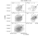
Figure 1: Integrated intensity maps ($\int T_{R}dv$) for the molecular transitions mapped in IRAS 05399–0121. The letters denote the position of the NH₃ core as listed by Harju et al. (1993) and the star symbol represents the IRAS point source. In this source the ammonia peak position and the IRAS source are at the same position. Contour levels and grey scale intensities for DCO⁺ and H¹³CO⁺ begin at 0.2 K km s^-1 and increase in steps of 0.2 K km s^-1. For CS and N₂H⁺ the contour levels begin at 0.4 K km s^-1 and increase in steps of 0.4 K km s^-1. C¹⁸O contour levels begin at 2.0 K km s^-1 and increase in steps of 0.4 K km s^-1. Peak values are listed in Table THE IONIZATION FRACTION IN DENSE MOLECULAR GAS II: MASSIVE CORES.

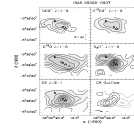
Figure 2: Integrated intensity maps ($\int T_{R}dv$) for various molecular transitions mapped in IRAS 05302–0537. Symbols are defined as given in Fig. 1. DCO⁺ and H¹³CO⁺ contour levels and grey scale intensities begin at 0.25 K km s^-1 and increase in steps of 0.25 K km s^-1. For CS and N₂H⁺ contour levels begin at 0.5 K km s^-1 and increase in steps of 0.5 K km s^-1. Peak values are given in Table THE IONIZATION FRACTION IN DENSE MOLECULAR GAS II: MASSIVE CORES. Contour levels for both the blue (solid line) and red (dashed line) outflow lobes begin at 0.2 K km s^-1 and increase by 0.2 K km s^-1. The high velocity blue emission was integrated from 6.4 to 7.6 km s^-1 and the red from 9.7 to 11.0 km s^-1.

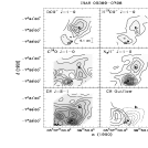
Figure 3: Integrated intensity maps ($\int T_{R}dv$) for various molecular transitions mapped in IRAS 05369–0728. Symbols are defined as given in Fig. 1. DCO⁺ and H¹³CO⁺ contour levels and grey scale intensities begin at 0.25 K km s^-1 and increase in steps of 0.25 K km s^-1. N₂H⁺ contour levels are 1.0 K km s^-1 to 10.0 K km s^-1 by steps of 1.0 K km s^-1. CS levels begin at 0.5 K km s^-1 and increase in steps of 0.5 K km s^-1. Peak values are given in Table THE IONIZATION FRACTION IN DENSE MOLECULAR GAS II: MASSIVE CORES. Contour levels for both the blue (solid line) and red (dashed line) outflow lobes are 0.4 K km s^-1 to 4.0 K km s^-1 by 0.3 K km s^-1. The high velocity blue emission was integrated from 2.0 to 3.7 km s^-1 and the red from 6.0 to 8.0 km s^-1.

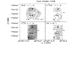
Figure 4: Integrated intensity maps ($\int T_{R}dv$) for various molecular transitions mapped in IRAS 05389–0756. Symbols are defined as given in Fig. 1, except for the open triangle which denotes the DCO⁺ peak that we call IRAS 05389–0756d in the text. Contour levels and grey scale intensities for DCO⁺ and H¹³CO⁺ begin at 0.2 K km s^-1 and increase in steps of 0.2 K km s^-1. C¹⁸O contour levels begin at 2.0 K km s^-1 and increase in steps of 0.4 K km s^-1. CS and N₂H⁺ levels begin at 0.4 K km s^-1 and increase in steps of 0.4 K km s^-1. Peak values are given in Table THE IONIZATION FRACTION IN DENSE MOLECULAR GAS II: MASSIVE CORES.

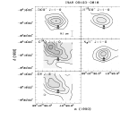
Figure 5: Integrated intensity maps ($\int T_{R}dv$) for various molecular transitions mapped in IRAS 05403–0818. Symbols are defined as given in Fig. 1. For DCO⁺ and H¹³CO⁺ maps, contour levels and grey scale intensities begin at 0.2 K km s^-1 and increase in steps of 0.2 K km s^-1. All other species begin at 0.4 K km s^-1 and increase in steps of 0.4 K km s^-1. Peak values are given in Table THE IONIZATION FRACTION IN DENSE MOLECULAR GAS II: MASSIVE CORES.

During March 1997 each source was mapped in the J $=1\rightarrow 0$ transitions of C¹⁸O and N₂H⁺, and the J $=2\rightarrow 1$ transition of CS using the Five College Radio Astronomy Observatory 14m antenna equipped with the 15-element focal plane array. The maps were full beam sampled and cover the entire region mapped in H¹³CO⁺ and DCO⁺ at NRAO. We used the autocorrelator spectrometer with 20 MHz bandwith and velocity resolutions of 0.11 km s^-1, 0.13 km s^-1, 0.12 km s^-1 for C¹⁸O, N₂H⁺, and CS respectively. All observations were obtained using frequency switching with a 4 MHz throw. In the contour maps (Figures 1 – 5) and for the analysis we convert all data to $T_{R}=T_{A}^{*}/\eta_{MB}$ using the efficiencies given in Table 2 (see Kutner & Ulich 1982).

3 Results

3.1 IRAS05399–0121a

Figure 1 presents integrated intensity maps of DCO⁺, H¹³CO⁺, N₂H⁺, C¹⁸O, and CS in the molecular core surrounding IRAS05399–0121. The morphology of the emission maps is similar, except that the N₂H⁺ emission appears to peak closer to the star than seen for other molecular species. The C¹⁸O integrated intensity map is somewhat larger than observed in the other tracers, and is most likely due to the lower critical density of this transition, n${}_{cr}\sim 10^{3}$ cm^-3, as compared to the other tracers which all have n${}_{cr}>10^{5}$ cm^-3 (e.g. Ungerechts et al. 1997). HWW list this core as a possible outflow candidate on the basis of ¹²CO emission widths greater than 10 km s^-1. Our CS spectra show some slight evidence for line wings, but there is no other evidence for an outflow in our data. This core has been observed previously and is listed as LBS30 in the Lada et al. (1991b) study and OriB9 in Caselli & Myers (1995). LBS30 has also been observed in dust continuum emission at both moderate ($\sim 30^{\prime\prime}$) and high ($\sim 12^{\prime\prime}$) resolution (Launhardt et al. 1996). The moderate resolution maps exhibit a clumpy structure with the strongest emission found near the IRAS source and a second weaker peak about $\sim 1^{\prime}$ to the southeast. The high resolution data show a single small condensation located within 20^′′ of IRAS05399, but within the IRAS error ellipsoid. The emission extent in our (lower resolution) molecular data encompasses all of the dust continuum emission. However, the molecular integrated intensity peaks appear to correspond with the second weaker dust continuum peak and not with the condensation directly associated with the young star.

3.2 IRAS05302–0537a,b

Contour maps of the integrated intensity from each of the lines observed towards IRAS05302–0537 are presented in Figure 2. The N₂H⁺ emission peaks directly to the north of the IRAS source and extends to the northeast. A similar distribution is observed for DCO⁺ and H¹³CO⁺. HWW designate the core to the northeast as a separate core (IRAS05302–0537b), but our lower resolution maps do not resolve a separate source. However, there are some observed emission differences. The C¹⁸O distribution encompasses all of the peaks found by other molecules, while the intensity of the other molecular species are highest near the IRAS source. IRAS05302–0537a does have an associated molecular outflow (Fukui et al. 1986), which is observed in the CS emission (shown on the bottom right-hand panel of Figure 2). However, because the outflow contribution to the CS emission is relatively weak it does not appreciably affect the overall CS distribution. The young star IRAS05302–0537 is also referred to as Orion A-W and a discussion of its properties can be found in Meehan et al. (1998).

3.3 IRAS05369–0728a,b

Figure 3 shows maps of the integrated intensity in the molecular gas near IRAS05369–0728 (also known as Haro 4-255). Towards this source Anglada et al. (1989) and HWW observed two NH₃ cores, with one sharply peaked condensation near the IRAS source and another less defined maximum 2^′ to the northwest. The distribution of our N₂H⁺ data closely resembles their ammonia observations. The second maximum away from the IR source is the starless core labeled as IRAS05369-0728b. For the other molecular ions, the structure also appears to be reasonably close to that seen in N₂H⁺. In contrast, the observed emission from both neutral species, CS and C¹⁸O, exhibits some differences from the ion distribution.

For CS the differences can be accounted for by the presence of an outflow from the IRAS source which contributes to the CS emission. An outflow associated with Haro 4-255 has been reported previously on the basis of CS J $1\rightarrow 0$ emission (Tatematsu et al. 1993b). The red and blue lobes of the outflow as observed by the J$=2\rightarrow 1$ transition of CS are shown in the bottom right-hand panel of Figure 3. This distribution is quite similar to that found in emission from the lower transition in Tatematsu et al. (1993b). If we remove the outflow contribution from the CS integrated intensity map by restricting the integration to the line core we find that the distribution is comparable to that observed in the other high dipole moment tracers (DCO⁺, H¹³CO⁺, N₂H⁺). The morphological differences between C¹⁸O and the other molecules are somewhat harder to reconcile and are most likely related to the differences in excitation requirements discussed in §3.1.

3.4 IRAS05389–0756a,b,d

Figure 4 presents the intensity maps for surveyed species towards IRAS05389–0756. For this source we do not have maps of the N₂H⁺ emission. While HWW detected 3 components in this core, our maps only cover two of these components (a and b). In NH₃ emission core (a) is a spatially broad condensation located near the star, while core (b) is a weak NH₃ maximum to the south. In our observations we see little evidence for the second core, and it is likely that core (b) is unresolved within our larger beam. Comparing the emission morphologies of H¹³CO⁺ and DCO⁺ we find distributions similar to ammonia, except that H¹³CO⁺ has an additional maximum 3^′ north of the IRAS source. This core was not detected in NH₃ emission because the maps did not extend this far to the north. We label this new starless core as IRAS05389–0756d.

Some of the C¹⁸O and H¹³CO⁺ spectra in this source show evidence for two velocity components centered near 4 and 5 km s^-1 (see Table 3). As the spatial and velocity resolution of the DCO⁺ observations are not high enough to resolve these components we have integrated over the entire line profile when calculating column densities (§4.1.2).

3.5 IRAS05403–0818a

Maps of the integrated intensity towards IRAS05403–0818 are presented in Figure 5. Again general agreement is observed between the various tracers. CS, DCO⁺, H¹³CO⁺, and N₂H⁺ exhibit a single emission peak $\sim 1^{\prime}$ north of the IRAS source. The NH₃ peak seems to disagree with the peak position observed for other tracers by $\sim 0.3-0.6^{\prime}$. However, closer examination of the ammonia emission distribution in HWW shows that the peak could also be assigned at $\sim 0.33^{\prime}$ north, close to the peak positions observed in our data. Similar to the other sources, C¹⁸O is distributed over a larger area and has a more extended peak. The C¹⁸O spectra have an additional component at $V_{lsr}\sim 5.7$ km s^-1, in contrast to the single component at $V_{lsr}\sim 3.0$ km s^-1 observed in other tracers. This extra C¹⁸O velocity component is probably due to a background cloud and has not been included in the intensity map in Figure 5. This source is also listed as containing a molecular outflow by HWW. Our CS maps show no evidence for any high–velocity gas.

4 Analysis

To derive electron abundances we utilize the [DCO⁺]/[HCO⁺] and [HCO⁺]/[C¹⁸O] column density ratios. Using these ratios requires reasonably high signal to noise for all relevant species as the relative errors will add in quadrature. In order to obtain the maximum signal to noise, we restrict our determination of molecular column densities and line parameters to the DCO⁺ emission peaks for each core. The integrated intensities and line parameters derived toward these positions for C¹⁸O, DCO⁺, H¹³CO⁺, and N₂H⁺are given in Table THE IONIZATION FRACTION IN DENSE MOLECULAR GAS II: MASSIVE CORES, and CS in Table 4. The offsets are relative to the central coordinate provided in Table 1. The resolution of the C¹⁸O observations were obtained with a slightly smaller beam size than those of H¹³CO⁺ and we have smoothed the C¹⁸O observations to a resolution of 65^′′. Since we have emission maps for each core – which contain additional information on electron abundances at the core edges – in Section 5.2 we will also examine a column density computed from averaging the integrated intensities away from the peak.

4.1 Physical Properties and Molecular Abundances

As discussed in detail in Paper I, the determination of electron abundances from observations of molecular ions requires information on the physical structure of the cloud, in particular the density and temperature of the gas probed by the respective tracers. These parameters are required to constrain the chemical model and also to calculate the molecular column densities from the integrated intensities.

4.1.1 Density and Temperature

The temperature of these cores, as traced by the symmetric top molecule NH₃, is typically $T_{k}\sim 15$ K (HWW) and we will adopt this value for our excitation and initial chemical analysis. Because the derivation of electron abundances relies on column density ratios derived from transitions with similar excitation requirements (see Table 2) our results are not highly sensitive to this choice.

To determine the density and column density in each core we have used a Large Velocity Gradient (LVG) code to calculate the radiative transfer of CS (Snell 1981). We ran a 20$\times$20 grid of models in density – column density space and then fitted our observed CS J = $2\rightarrow 1$ and J = $3\rightarrow 2$ observations to the grid of models using a $\chi^{2}$ minimization routine. The densities in the grid ranged from $10^{4}$ to $10^{6}$ cm^-3 and the column densities per velocity interval, $N/\Delta V$ from $10^{11}$ to $10^{14}$ cm^-2 (km s^-1)^-1. We ran two grids: one for T_k = 15 K and one for 25 K to allow for slightly hotter gas. The best fit models are presented in Table 5 and show that the densities of the gas probed by CS are typically $\sim 10^{5}$ cm^-3.

The density uncertainty is also listed in Table 5 and this value is based on the observed baseline rms noise, and an assumed systematic uncertainty of 30%. One concern is that the density is derived on the basis of two adjacent rotational transitions that may not be sensitive to material with a density much greater than the critical density of the $J=3\to 2$ transition. We can attempt to address these questions by comparison to other measurements in the literature. One core (IRAS05399) was included in a multitransitional CS study in Lada, Evans, & Falgarone (1997) who detected emission from the $J=5\to 4$ transition. They derive a density of n${}_{H_{2}}$ $=2\times 10^{5}$ cm^-3, analogous to our result. However, Launhardt et al. (1996) derive a density of $>$ 2.9 $\times 10^{7}$ cm^-3 on the basis of 1.3mm dust continuum observations of the same object. Another dust continuum study of the gas associated with IRAS05389 derives a density for the envelope (r $>10^{\prime\prime}$) of $\sim 10^{5}$ cm^-3 (Zavagno et al. 1997; S72 in their notation), similar to our value. The large difference between CS and dust continuum density measurements in IRAS05399 may be due to the higher resolution of the dust continuum observations ($\sim 12^{\prime\prime}$), which will result in greater sensitivity to warmer, denser, material close to IRAS05399. Our lower resolution molecular data ($60-80^{\prime\prime}$) using transitions with low excitation energies may only probe outer layers which have lower (and more average) densities.

4.1.2 Molecular Column Densities and Ratios

Column density estimates for CS have been made on the basis of the non-LTE excitation model described in the preceding paragraph. For C¹⁸O, DCO⁺, H¹³CO⁺, and N₂H⁺ we assume that the emission is optically thin and that the excitation temperature is greater than the background. As in Paper I we initially compute column densities using LTE. However, at the densities of these cores, n${}_{H_{2}}\sim 10^{5}$ cm^-3, the level populations will not be in LTE and the column densities derived via observations of low–J levels will be overestimated. We have used a statistical equilibrium model at n${}_{H_{2}}=10^{5}$ cm^-3 and $T_{k}=15$ K to estimate the non-LTE correction factor for each species assuming optically thin emission. The non-LTE correction factors are 0.96 for C¹⁸O, 0.51 for DCO⁺, 0.58 for H¹³CO⁺, and 0.65 for N₂H⁺. The column densities corrected using the beam efficiencies listed in Table 2, and corrected for non-LTE populations, are listed in Table 7. To estimate the column density of HCO⁺ and CO we have used [¹²C]/[¹³C] $=60$ and [¹⁶O]/[¹⁸O] $=500$.

In the above analysis we have assumed that the emission is optically thin. We have some support for this assumption from observations of HC¹⁸O⁺ J $=1\rightarrow 0$ ($\nu=$ 86.75433 GHz) at two positions in IRAS05369-0728. These observations were obtained at the H¹³CO⁺ peak and at $\sim 0.75^{\prime}$ east of that position. For these positions we find 1$\sigma$ detection limits of $\int T_{R}dv$(HC¹⁸O⁺) $<0.12$ K km s^-1 and $<0.02$ K km s^-1 respectively. Using the isotope ratios listed above, the opacity of H¹³CO⁺ is $<1$ for both positions. Thus, the H¹³CO⁺ emission for this core, and by extension the others, is likely to be thin. For C¹⁸O and DCO⁺ we have no independent information on the opacity. However, the DCO⁺ and C¹⁸O lines are typically gaussian shaped with $T_{R}<3.0$ K, which is below the estimated temperature of 15 K, suggesting that the emission is thin.

4.2 Chemical Model

To derive ionization fractions we have adopted the method described in Paper I. In particular, we vary both physical parameters and atomic abundances in the chemical model to match observed abundances of molecular ions and column density ratios and derive electron fractions. The chemical model is described in Bergin & Langer (1997) and uses the pure gas-phase reaction network from Millar, Farquhar, & Willacy (1996).

The physical parameters varied are the density ($n_{H_{2}}$), gas temperature ($T_{gas}$), cosmic ray ionization rate of H₂ ($\zeta_{H_{2}}$), visual extinction ($A_{V}$), and the enhancement, $\chi$, of the local ultra-violet (UV) radiation field above the normal interstellar value of 1.6 $\times 10^{-3}$ erg cm^-2 s^-1 (Habing 1968). The density in these sources is constrained by the emission analysis discussed in Section 4.1 to lie within a range of $n_{H_{2}}=3-30\times 10^{4}$ cm^-3, and we adopt $n_{H_{2}}=10^{5}$ cm^-3 for our analysis. The visual extinction within a C¹⁸O beam can be determined using the C¹⁸O column densities provided in Table 7. If we assume that [C¹⁸O]/[H₂] $=5.0\times 10^{-7}$ (based on direct H₂ and CO measurements in Lacy et al. (1994) and [¹⁶O]/[¹⁸O] = 500), and N(H₂) $=10^{21}A_{V}$ then extinctions range from $A_{V}=4-12$ mag at the chosen positions. We have adopted a value of $A_{V}=7.5$ mag for our analysis, which is near the middle of this range. On the basis of the ammonia observations we adopt $T_{k}=15$ K, but we allow for the temperature to be as high as 30 K in the chemical calculations. Since the cores are located in a region of massive star formation where the radiation field could be higher than average we examine changing the UV enhancement factor and the visual extinction (discussed in §5.2).

In Paper I, to constrain the range of potential cosmic ray ionization rates, we balanced the heating due to a variable cosmic ray flux with the molecular line cooling calculations of Neufeld, Lepp, & Melnick (1995) and Goldsmith & Langer (1977) for a cloud temperature of 10 K. A similar analysis allowing for temperatures as high as 15–20 K suggests that ionization rates between $\zeta_{H_{2}}\sim 1-15\times 10^{-17}$ s^-1 will heat the gas to temperatures that lie within the allowed range. We have therefore performed model runs with $\zeta_{H_{2}}=$ 1, 5, 10, and 15 $\times 10^{-17}$ s^-1. This was done for all permutations of varied parameters (i.e. density, temperature, initial atomic abundances). From these models we found that $\zeta_{H_{2}}=5\times 10^{-17}$ s^-1 best reproduced the observations and we have adopted this value for the remainder of this paper. This value of $\zeta_{H_{2}}$ is consistent with the value found in Paper I for low mass cores.

Additional parameters in our model are the initial abundances of carbon, oxygen, nitrogen, and heavier “metal” atoms. As in Paper I we alter the initial chemical abundances from fiducial values which represent abundances typically used for theoretical chemical models. These fiducial conditions have C, O, and N with mild depletions with respect to solar (factor of 2–3), and the heaver species (Mg, Fe, S….) depleted by several orders of magnitude from solar values. Thus the fiducial set of initial atomic abundances are already depleted from Solar and we will raise and lower our initial model abundances from these fiducial values. We use the same fiducial set of abundances as given in Paper I. For each set of parameters (density, temperature, cosmic ray flux, etc.) the abundances of metal ions are varied from 1/10 to 150 times the normal value. For a given cosmic ray ionization rate this will effectively raise and lower the ionization level respectively. Upon comparison with observations we found that only a small range of factors between 2 – 10 times fiducial values is required. To account for variable depletions in the carbon and oxygen pools the carbon and oxygen abundances were also varied from 0.5 to 1.2 times the fiducial values. We also varied the nitrogen abundance and found that it does not affect the derived $x_{e}$.

In summary, perhaps one of the greatest uncertainties in the calculation of theoretical chemical abundances is the large number of variables involved in the calculation. In this work we have attempted to avoid this obstacle by computing over 600 model runs covering as many permutations of the parameter space as possible. Where possible we have used observations to constrain particular variables. In the following section we demonstrate that a reasonable range of these parameters can cover the observed spread in the data – and allow for an estimation of electron abundances in these cores. A compilation of the chosen model parameters for our “best fit” model is provided in Table 6.

4.3 Electron Abundances

Figure 6 plots the abundance of HCO⁺ relative to CO against the deuterium fractionation ratio: [DCO⁺]/[HCO⁺] for our sample of Orion cores (as open diamonds). Also shown as solid dots are the same ratios for low mass cores taken from Paper I. Comparing our data to the low mass cores shows general agreement in the same overall range of HCO⁺ abundances. However, the level of fractionation in deuterium is slightly different: the majority of massive cores have very low deuterium fractions (log₁₀([DCO⁺]/[HCO⁺]) $<-1.45$). Moreover, the two cores with the lowest fractionation ratios have outflows that are traced by CS emission.

Figure 7 overlays the best-fit chemical models on the Orion core data (same axes as Figure 6). Vertical lines in Figure 7 indicate the model temperature, whereas the horizontal contours denote the log of electron abundance (log${}_{10}x_{e}$). This family of models has $\zeta_{H_{2}}=5\times 10^{-17}$, $n_{H_{2}}=10^{5}$ cm^-3, carbon and oxygen abundances depleted by 20% from the nominal values (see Table 6). The cores containing stars are plotted as filled circles and starless sources are open circles. As in Paper I the vertical spread in the data is accounted for by variations in metal ion abundances. The line for log${}_{10}(x_{e})=-7.3$ in Figure 7 corresponds to 2 times the fiducial metal abundances and the line for log${}_{10}(x_{e})=-6.9$ corresponds to 10 times the fiducial values. Thus the range of our observations requires only a small variation in metal abundances. As the fiducial abundances are already heavily depleted from the observed abundances in diffuse clouds (and even more so from solar values) our results still require highly depleted metals. The electron abundances derived for the surveyed Orion cores are determined on the basis of the best fit model shown in Figure 7. Values are given in Table 7 along with the maximum and minimum abundances derived from the model and the 1 $\sigma$ observational errors in the ratios.

There is one major difference between the models presented here and those constructed for low mass cores (Paper I). The range of densities observed in low mass cores allowed us to fit models with constant temperature and a small range of C and O depletions (0.5 to 1.2 times the fiducial values). However, the densities in the massive cores are constrained to a fairly narrow range, with most falling around 10⁵ cm s^-1 (Table 5). At this density models similar to those presented in Paper I are unable to reproduce the low [DCO⁺]/[HCO⁺] ratios observed in some cores. For a fixed temperature the lowest ratios require high carbon and oxygen abundances, to a degree that is inconsistent with observed depletions towards diffuse clouds. Moreover the Orion cores observed here are much denser than diffuse clouds and should, if anything, show larger depletions.

Temperature variations within the sample of massive cores offer a simple solution to account for the observed differences. The main reaction that forms H₂D⁺ (and eventually DCO⁺) is:

$${\rm H}^{+}_{3}+{\rm HD}\rightleftharpoons{\rm H}_{2}{\rm D}^{+}+{\rm H}_{2}.$$ (1)

The forward reaction (formation of H₂D⁺) is favored at low temperatures, but once the temperature becomes greater than $\sim$20 K the reverse reaction will begin to contribute significantly and the [DCO⁺]/[HCO⁺] ratio will be lowered. Therefore, we account for the range of [DCO⁺]/[HCO⁺] ratios in Figure 7 by varying the temperature from 15 K to 30 K (vertical lines). We believe this explanation is plausible because the cores that contain stars and molecular outflows have the lowest fractionation ratios, whereas the starless cores have [DCO⁺]/[HCO⁺] ratios close to those observed in the colder low mass cores (Paper I). A similar analysis of deuterium fractionation in a wide range of cores by Wootten et al. (1982) also suggests that temperature variations are necessary to account for the observed differences.

Carbon and oxygen depletion is still a variable in the model calculations. As demonstrated in Paper I changes in the carbon and oxygen depletion can alter the electron fraction (a depletion of 25% from the normal values raises $x_{e}$ by $\sim$25%). The best fit to our data requires an additional depletion of 20% from the nominal values of [C]/[H₂] = $1.46\times 10^{-4}$ and [O]/[H₂] = $3.52\times 10^{-4}$. However, our data are consistent with C and/or O depletions of 50% and enhancements as high as 125%, provided that the temperature is still a variable. Chemical models of the Orion ridge near the Trapezium cluster, a region that is quite unique compared to the rest of the Orion cloud, suggest that oxygen atoms might be more depleted than carbon atoms (giving higher C/O ratios: Bergin et al. 1997a). In addition a recent compendium of oxygen depletion measurements from the Goddard High Resolution Spectrometer suggests that the total oxygen abundance is homogeneous in the solar vicinity and is two-thirds of the solar value (Meyer, Jura, & Cardelli 1998). Given the best fit C and O abundances, and the range of allowed depletions in the models, our results do not disagree with the chemical models of the Orion ridge or with the recent oxygen measurements.

5 Discussion

5.1 Comparison with Previous Models

Within the observational and theoretical errors (estimated to be a factor of 4; see discussion in §5.3) our electron abundances are consistent with those estimated by Wootten et al. (1982). However, our paper uses a direct comparison to chemical models, with associated improvements in reaction rates. Another study observed several molecular ions and neutrals, and with comparison to current equilibrium chemical models, derived electron abundances in several massive star forming cores (de Boisanger et al. 1996). Their chemical models are similar to ours in the sense that the cosmic ray flux is constant for an entire cloud (or complex), but their sources contain a significantly larger amount of mass and are located near O and B clusters. Our approach of fixing the ionization rate is different from that found in Caselli et al. (1998) who derived electron abundances for a sample of low mass cores (mostly in Taurus and Ophiuchus). Caselli et al. (1998) used the cosmic ray ionization rate as a true variable parameter in their analysis and account for the spread in [DCO⁺]/[HCO⁺] and [HCO⁺]/[CO] ratios through an intrinsic variation of the cosmic ray flux from core to core. Our analysis takes the flux of cosmic rays as a variable only to fit the entire sample. Slight differences in temperature between cores can account for the changes in deuterium fractionation between the different cores. Since our small sample of cores is located solely in the Orion complex, it is likely that the exteriors of these cores are bathed in a similar cosmic ray flux. A single value for the cosmic ray flux for a region several parsecs in size is also supported by the large-scale consistency of the diffuse gamma-ray emission, which is believed to originate from cosmic ray interactions with matter, with the large-scale distribution of the ISM (see Bertsch et al. 1993 and references therein).

An important source of concern in our models is the requirement that metal ions vary in abundance among our small sample of cores by a factor of 6. As noted in §4.2 this small variation still implies that metal abundances are heavily depleted from diffuse cloud values. Such a variation could be found if these cores have slightly different density structures and formation histories. In this regard it is encouraging that the electron abundances and predicted metal depletions in the two sources with multiple cores are quite similar. Another complication is that the non-linear character of chemical equations has been shown to give rise to multiple solutions with high- and low-ionization phases (Le Bourlot, Pineau des Forêts, & Roueff 1995). These solutions are found to be dependent on the initial conditions. Thus, the fractional ionization may not be uniquely determined from the molecular column density ratios used here. However, in our models we have examined a large fraction of the parameter space (abundances of metals, cosmic ray ionization rate, temperature, and density). In all, over 1200 models were run for this paper and in Paper I to find the the best match to the data. In no case was a bistable solution found and our results are consistent with the low-ionization phase (see Plume et al. 1998). Finally, the non-inclusion of gas-grain interactions could be important. For a detailed discussion of these effects and other possible sources of electrons the reader is referred to the discussion in Paper I.

5.2 The Effect of the Radiation Field

In terms of electron abundances and the radiation field there are two possible effects. One concern is that the local radiation from an associated young star may heat the surrounding molecular envelope and produce a gradient in the deuterium fractionation along the line of sight. In contrast the HCO⁺ abundance will not be as strongly affected. Using Figure 7 we can attempt to quantify these effects. Along a line of constant [HCO⁺]/[CO], the derived electron fraction increases by a factor of 1.6 as the deuterium fractionation ratio declines. Thus, a gradient in D-fractionation will result in an overestimation of the actual electron abundance.

For most cases we have avoided this particular concern by performing our analysis along lines of sight away from the stellar position. The analysis for one source, IRAS05389–0756a, is performed near the position of the IRAS source and it is possible that this could affect our determination of the electron abundance. If we examine Figure 7 the [DCO⁺]/[HCO⁺] ratio for IRAS05389 core (a), which is near the IR source, and core (d), which is apparently unassociated with star formation, are nearly identical. This suggests that, for this source at least, such line of sight effects may not be a dominating factor. To probe this question further we can compare the [DCO⁺]/[HCO⁺] ratio computed at the stellar position with a single position away from the source for all surveyed cores. We find that, on average, the change is 20% in the direction of lower fractionation. A typical statistical error in the D/H ratio is $\sim 30$% which suggests that, on average, this effect is not important at the observed spatial resolution. One source, IRAS05302–0537, one of the more luminous stars in our sample ($L_{IR}=57L_{\odot}$), shows a 67% decrease. Thus, there is some (inconclusive and limited) evidence of this effect. A larger sample of sources and data with greater spatial resolution and sensitivity will be required to examine this question in more detail.

A second potential effect is from the external radiation field. McKee (1989) showed that for a homogeneous gas layer illuminated by the normal interstellar radiation field, cosmic ray ionization and photoionization contributed equally at $A_{V}\sim 4$. We have investigated the effects of the radiation field on our chemical calculations by lowering the visual extinction or, equivalently, raising the external UV field. Since these cores are located in the Orion cloud, which have several local sources of intense radiation (e.g. Genzel & Stutzki 1989), we have investigated raising the UV radiation field by a factor of 500. We find that our results are unaltered. Raising the UV field to $\chi=500$ corresponds to lowering the visual extinction to $A_{V}\sim 2-3$ (depending on the molecular photoabsorption cross-section), and at these depths CO molecules are still partially shielded from radiation. It is important to note that our models do account for the self-shielding of CO.

We have further investigated the effect of the radiation field by comparing the [DCO⁺]/[HCO⁺] ratio and the H¹³CO⁺ abundances in the core edges to those found in the center. The separation between the core edges and center is defined as the contour at which the DCO⁺ J = $1\rightarrow 0$ integrated intensity is equal to half the peak value. For a particular molecule, all spectra that lay in the “edge” region ($\int{T_{R}dV(DCO^{+})}<1/2\int{T_{R}dV_{peak}}$) were combined to produce a single “edge” spectrum whereas those that fell in the “center” were combined to produce a single “center” spectrum. In this fashion, we obtained average “edge” and “center” spectra for each molecule in each of the cores in our sample. This analysis was performed on IRAS05399–0121 and IRAS05302–0537, since these cores are centrally condensed and have enough spectra to construct meaningful averages. We find that, in IRAS05399–0121, the [DCO⁺]/[HCO⁺] ratio increases by only 0.1 in the log between the edge to the center, and the [HCO⁺]/[CO] ratio increases by less than 0.3 in the log. In IRAS05302–0537, both the [DCO⁺]/[HCO⁺] and [HCO⁺]/[CO] ratios increase by only 0.1 in the log as one goes from the edge to the center. Inspection of Figure 7 shows that these small changes in the abundance ratios lie well within our observational error bars and have a minimal effect upon the derived electron abundance. Thus, we find no difference in the deuterium fraction or the H¹³CO⁺ abundance between the low visual extinction core edges and the core centers. The ionization fraction implied by this result depends on the unknown density structure of these cores. For a constant density (and temperature) our models will predict similar ionization levels between edge and center of the maps. If these cores have a power-law density profile as found for some low mass cores (Goldsmith & Arquilla 1985; Ward-Thompson et al. 1994) and suggested by Zavagno et al. (1997) for IRAS05389–0756, then the model predicts a slightly higher level of ionization at the core edges. However, for both scenarios cosmic ray ionization provides the main source of electrons.

In order to more carefully investigate the effects of photoionization we can utilize the model of Jansen et al. (1995) who examined the depth dependent chemistry of IC63, which has a B star located $\sim 1$ pc away. This work includes a detailed treatment of the observed UV field of the B star, and its coupling to the photodissociation rates for various molecules. In their model, the abundance of HCO⁺ is $\sim 10^{-11}$ near the core edges, due to the increased abundance of photo-produced electrons. At larger depths ($A_{V}>$ 4) the abundance increases to $\sim 10^{-9}$. Since our results show no evidence for a decline in the HCO⁺ abundance we conclude that we are tracing gas that is shielded from UV radiation and ionized primarily by cosmic rays. The lack of abundance variation from the edge to the center is similar to recent measurements of abundances across the M17 molecular cloud/ionization front interface where molecular abundances show little variation despite large changes in the radiation field (Bergin et al. 1997b).

5.3 Electron Abundances and Star Formation

It is worthwhile to compare the electron abundances between our sample of massive and low mass objects. In order to extend our study towards even more massive cores we use previous studies in the literature. Wootten et al. (1982) surveyed many sources for emission from DCO⁺, H¹³CO⁺, and ¹³CO. We have used their raw data from NGC1333 and in Serpens (Ser MC1 in their notation) to derive column densities and, with comparison to our models, electron abundances. We find that $x_{e}=4\times 10^{-8}$ in NGC1333 and $x_{e}=5\times 10^{-8}$ in Serpens. We can also draw upon the recent work of de Boisanger et al. (1996) who examined electron abundances in denser, very massive sources: W3 IRS5 ($x_{e}=1\times 10^{-8}$) and NGC2264 ($x_{e}=5\times 10^{-9}$). Finally, we compare the observations of Bergin et al. (1997a) in the OMC-1 core to our chemical models to obtain $x_{e}=2\times 10^{-8}$.

Before we compare the electron abundances between our work here and in Paper I with those of de Boisanger et al. (1996) it is worthwhile to estimate the total uncertainty in the derived electron fraction. In Table 7 we provide an estimate of the minimum and maximum electron abundance that is consistent with the statistical errors in the observed column density ratios. The average range is $\Delta$log₁₀($x_{e})=0.3$, which suggests that the uncertainty is, roughly, a factor of $\sim$1.4. This range does not include any systematic error that might be introduced by our assumptions with regard to the physical parameters such as the density and temperature. For the massive cores sampled here, the uncertainty in the determined density, including statistical and systematic effects, is typically a factor of $\leq$3 (see Table 5). This produces a factor of two uncertainty in the derived ionization fraction. For the temperature, if we assume that the allowed range is between 15 and 25 K then this is an additional factor of 1.5. Therefore, with the additional assumption that the cosmic ray ionization rate is the same for each core (see §5.1), the total uncertainty in the derived electron fraction is a factor of $\sim$4. The same reasoning applies to the analysis in Paper I, while de Boisanger et al. (1996) find that their chemical model predictions are within a factor of two of the observed abundances of 7 ions.

Perhaps the most meaningful comparison between electron abundances among the overall sample of cores would compare the level of ionization to the density of each core. However, there is no comprehensive examination of the density using similar models, observations, and methods for the entire range of objects. The densities of the very massive cores (e.g. OMC-1) have been determined via excitation analyses of CS, H₂CO, and HC₃N, with values ${}_{\sim}^{>}10^{6}$ cm^-3 (e.g. Mundy et al. 1985; Plume et al. 1997; Bergin, Snell, & Goldsmith 1997). The massive cores studied in this work have lower densities, $n_{H_{2}}\sim 10^{5}$ cm^-3, from our CS analysis. However, the low mass cores have not been systematically studied using these techniques, although Caselli & Myers (1995) show that for a given radius low mass cores have smaller densities by about a factor of three (i.e. massive cores are larger and denser).

Since the density is not consistently derived for each source we have opted to use the total H₂ column density along the line of sight. The H₂ column density is determined using N(C¹⁸O), and an assumed fractional abundance of $5\times 10^{-7}$. H₂ column densities for W3 IRS5 and NGC2264 are taken from de Boisanger et al. (1996), while for OMC-1 we use the C¹⁸O column densities in Bergin et al. (1997a). The electron abundance shown as a function of N(H₂) is presented in Figure 8. Examining Figure 8, the abundances for the low mass cores show a large degree of scatter, with a median value of $<x_{e}>\sim 10^{-7}$. The massive cores (along with Serpens and NGC1333) overlap with the low mass sources, but are more clustered with a lower median electron abundance of 6 $\times 10^{-8}$. Given the estimated uncertainties, which will be reduced by $\sqrt{N}$ (N $=$ the number of cores) for the median, and the small number of data points for massive cores, the differences between these two samples are only suggestive. However, there is a significant difference in the ionization fraction between the very massive (and densest) cores (W3, OMC-1, and NGC2264) and the low mass cores. These results suggest that the regions with the highest column and volume densities also have lower electron abundances, as would be expected from the conventional picture of cosmic ray ionization. However, these results must be viewed with caution as there are only 3 data points for very massive sources and the electron abundances for these sources were derived from a different (although equally valid) model. It is noteworthy that there appears to be no difference in the ionization fraction between cores directly associated with star formation and cores without any activity.

5.4 Ion-Neutral Coupling in Massive Cores

In Paper I we examined the question of the ion-neutral coupling in low mass cores in terms of the wave coupling parameter. The wave coupling parameter, $W$, is defined as the ratio of the core size, $R$, to cutoff wavelength $\lambda_{0}$. The cutoff wavelength is defined by $\lambda_{0}=\pi v_{A}/[n_{i}<\sigma_{in}v>]$, where $v_{A}$ is the Alfvén speed, $n_{i}$ the ion density, and $<\sigma_{in}v>$ the ion-neutral collision coefficient. If W $\gg 1$ the field and gas are coupled over a large range of size scales. For W $\ll 1$ the ions are decoupled from the field and MHD waves are suppressed (see Paper I for a more comprehensive discussion).

The ionization fraction is determined by the balance of cosmic ray ionization and recombination, along with any contribution from metal ions with low ionization potential and longer recombination timescales. The relation between these values can be expressed as

$$x_{e}=C_{i}n_{H_{2}}^{-1/2}\zeta_{H_{2}}^{1/2}$$ (2)

where $C_{i}$ is a constant that contains the relative contributions of molecular ions and metals to the ionization balance. McKee (1989) derives $C_{i}=3.2\times 10^{3}$ cm^-3/2s^1/2 for an idealized model of cosmic ray ionization. In Paper I we derived a value of $C_{i}=2.0\times 10^{3}$ cm^-3/2s^1/2. If we use our average electron abundance of $8\times 10^{-8}$ and density of 10⁵ cm^-3, we find, for the massive cores in Orion, a value of $C_{i}=3.6\times 10^{3}$ cm^-3/2s^1/2. Considering the error in the electron fraction the difference between the value derived here and for low mass cores is not significant.

For cores which are ionized primarily by cosmic rays and are dominated by non-thermal motions, the wave coupling parameter is independent of density and can be expressed as:

$$W=\frac{C_{i}<\sigma_{i}v>}{\pi}\left[\frac{10\zeta_{H_{2}}}{4\pi mG}\right]^{1/2}$$ (3)

where $<\sigma_{i}v>=1.5\times 10^{-9}$ cm³s^-1, and $m$ is the mean molecular mass per particle. The equation is listed for the case of maximum turbulence as appropriate for massive cores. Both of these conditions, high non-thermal width and cosmic ray ionization, are satisfied for the massive cores in our study and using our best fit value of the ionization rate, $\zeta_{H_{2}}=5\times 10^{-17}$ s^-1, gives $W=20$.

Thus the field-neutral coupling W of the seven massive cores analyzed here is similar to, or perhaps slightly larger than, that deduced for the 20 low mass cores in Paper I (W = 11). For both samples, the coupling is “marginal,” i.e. strong enough to allow propagation of MHD waves, but weak enough for some wave damping to occur (Martin, Heyvaerts, & Priest 1997, Nakano 1998, Myers & Lazarian 1998). This suggests that both low mass and massive cores are more vulnerable to fragmentation and dissipation of their turbulence than are their lower-density, better-coupled environs (Myers 1997).

However, the massive cores considered in this paper appear better able to form stellar groups and clusters than the low mass cores in Paper I, for two reasons. First, the massive cores can be “clumpier” than low mass cores, because they have a greater ratio of turbulent to thermal speeds than do the low mass cores (Myers 1998). Second, the typical massive core is a factor of $\sim$2 larger than the typical low mass core, so the massive core has more high-density gas and more volume available in which to form stars, than does the typical low mass core. It will be useful to extend the observations and analysis presented here to more “very” massive regions forming OB stars and rich clusters.

6 Conclusions

We have mapped the emission of three molecular ions (DCO⁺, H¹³CO⁺, and N₂H⁺) and two neutral species (CS and C¹⁸O) in massive dense cores. In all we survey 5 cores that are currently associated with star formation and 2 that are starless. These cores are located in the L1630 and L1641 star forming regions, and are more massive, turbulent, and larger than the sample of low mass cores subject to a similar study in Paper I. We have used these observations to derive electron abundances using the same method and chemical model as applied to the low mass cores in Paper I. The principal results of this study are:

1) With use of observations to constrain variables in the chemical calculations, we have constrained the electron fraction in our sample to lie within a small range –6.9 $<$ log₁₀($x_{e}$) $<$ –7.3, with an average value of –7.11 $\pm 0.15$. These values are consistent with previous analyses of ionization fractions in other star forming regions. No difference is found between the electron abundances inferred for cores with and without stars. However, the cores directly associated with stars and molecular outflows have lower levels of deuterium fractionation, which can be attributed to differences in temperature between the various sources.

2) Among our sample of cores we have searched for differences in the ionization level between the core edges and center. For the two cores that we examined in detail, the observed levels of deuterium fractionation and HCO⁺ abundances do not change with position. The exact value of ionization fraction implied by the constant ratios depends quite critically on the unknown density/temperature structure of these sources. However, the lack of variation suggests that even the core edges probed by these high dipole moment molecules are shielded from ultra-violet radiation and cosmic rays remain the primary source of ionization.

3) Using the previously determined electron fractions in low mass cores forming single isolated stars, and other values for very massive cores associated with O and B stars, we have systematically examined electron abundances over a wide spectrum of star formation activity. The very massive sources, such as OMC-1 or W3, have ionization fractions typically an order of magnitude below those estimated for low mass cores where $<x_{e}>\sim 10^{-7}$.

4) The issue of ion-neutral coupling is examined as a function of core properties. We find that the size of the decoupled region is larger for more massive cores; thus massive cores have a greater amount of mass with lower field-gas coupling available to form stars.

We are grateful to K. Strom and L. Allen for making available their near-infrared data in L1641. We also thank P. Caselli and M. Walmsley for several discussions on the topic of electron abundances and A. Dalgarno for discussions on cosmic ray ionization. E.A.B. and R.P. thank the AAS for a small research grant to support this work and also acknowledge support from NASA’s SWAS contract to the Smithsonian Institution (NAS5-30702). P.C.M. and J.P.W. acknowledge partial support from NASA Origins of Solar Systems Program grant NAGW-374.

Table 1: Map Central Positions

Source	$\alpha(1950)$	$\delta(1950)$
IRAS05399–0121a	05h39m55.1s	–01∘21′24′′
IRAS05302–0537a	05 30 15.8	–05 37 32
IRAS05369–0728b	05 36 51.1	–07 25 34
IRAS05389–0756a	05 38 56.6	–07 56 40
IRAS05403–0818a	05 40 23.3	–08 18 26

Table 2: Observed Transitions and Telescope Parameters

Molecule	Transition	$\nu$(GHz)	$E_{u}$ (K)	Telescope	$\theta_{MB}$	$\eta_{MB}$
DCO+	$J=1\rightarrow 0$	72.039331	3.46	NRAO	80′′	0.93
H13CO+	$J=1\rightarrow 0$	86.754329	4.16	NRAO	67′′	0.91
N2H+	$J=1\rightarrow 0$	93.1737	4.47	FCRAO	56′′	0.51
CS	$J=2\rightarrow 1$	97.981011	2.35	FCRAO	53′′	0.50
C18O	$J=1\rightarrow 0$	109.782182	5.27	FCRAO	47′′	0.46
CS	$J=3\rightarrow 2$	146.969049	7.05	NRAO	43′′	0.75

Table 4: CS Line Parameters

Source	J $=2\rightarrow 1$			J $=3\rightarrow 2$
	TR (K)	Vlsr (km s-1)	$\Delta v$ (km s-1)	TR (K)	Vlsr (km s-1)	$\Delta v$ (km s-1)
IRAS05399–0121a	1.08(0.10)	9.0	1.1	1.32(0.06)	9.0	1.2
IRAS05302–0537a	0.82(0.10)	8.5	2.3	1.38(0.06)	8.3	1.8
IRAS05369–0728a	1.00(0.10)	4.3	0.8	1.17(0.07)	4.6	3.5
IRAS05369–0728b	0.92(0.07)	5.0	1.5	0.91(0.06)	4.9	1.4
IRAS05389–0756a	0.56(0.09)	4.7	1.4	0.42(0.06)	4.6	1.2
IRAS05403–0818a	1.09(0.14)	3.2	0.7	1.14(0.06)	3.1	1.2

Table 5: Core Densities and CS Column Densities

	Tk = 15 K		Tk = 25 K
Source	log10 n${}_{H_{2}}$	log10 N(CS)	log10 n${}_{H_{2}}$	log10 N(CS)
IRAS05399–0121a	5.2(0.3)	13.2(0.2)	5.0(0.3)	13.2(0.3)
IRAS05302–0537a	5.6(0.4)	13.2(0.3)	5.4(0.3)	13.1(0.3)
IRAS05369–0728a	5.2(0.4)	13.4(0.5)	4.9(0.4)	13.4(0.6)
IRAS05369–0728b	4.9(0.5)	13.3(0.3)	4.7(0.6)	13.2(0.4)
IRAS05389–0756a	4.5(1.2)	13.3(1.5)	4.1(2.0)	13.2(0.3)
IRAS05403–0818a	5.0(0.4)	13.2(0.3)	4.7(0.5)	13.2(0.4)

Table 6: Adopted Model Parameters

Parameter	Value
$\zeta_{H_{2}}$	5 $\times 10^{-17}$ s-1
$n_{H_{2}}$	1.0 $\times 10^{5}$ cm-3
$T_{k}$	$15-30$ K
$A_{V}$	7.5 mag
$\chi$	1.0
He	0.28
HD	2.8 $\times 10^{-4}$
C+	1.17 $\times 10^{-4}$
O	2.82 $\times 10^{-4}$
N	4.28 $\times 10^{-5}$
M+	2 – 10 M${}^{+}_{0}$

Table 7: Molecular Column Densities and Electron Abundances

Source	log10 N(DCO+)	log10 N(H13CO+)	log10 N(N2H+)	log10 N(C18O)	$x_{e}$	Min	Max
IRAS05399–0121a	12.15(11.2)	11.84(11.1)	12.60(11.4)	15.76(14.3)	–6.87	–6.74	–7.03
IRAS05302–0537a	12.21(11.1)	12.01(10.9)	12.84(11.3)	15.48(14.2)	–7.22	–7.14	–7.31
IRAS05369–0728a	11.95(11.1)	11.87(11.0)	12.61(11.4)	15.35(14.3)	–7.18	–7.05	–7.33
IRAS05369–0728b	12.22(11.2)	11.78(11.1)	12.59(11.3)	15.43(14.3)	–7.28	–7.15	–7.40
IRAS05389–0756a	12.06(11.0)	11.73(11.0)	$\cdots$	15.51(14.1)	–7.00	–6.83	–7.17
IRAS05389–0756d	12.15(11.1)	11.84(11.1)	$\cdots$	15.58(14.5)	–7.04	–6.86	–7.20
IRAS05403–0818a	12.11(11.1)	11.87(10.9)	12.42(11.5)	15.38(14.2)	–7.20	–7.08	–7.31

Figure 6: Column density ratios for the low mass cores surveyed in Paper I and the massive cores in the current study.

Figure 7: Contours of ionization fraction as a function of column density ratio. The logarithm to base 10 of the electron fraction is labeled in each plot along the right hand side of the contours. The model is for a density of n${}_{H_{2}}=10^{5}$, $\zeta_{H_{2}}=5\times 10^{-17}$ s^-1, $A_{V}=7.5$ mag, and the normal interstellar radiation field (see Table 6 for listing of other parameters). Variations in $y$, the gas kinetic temperature in the model, is labeled along the upper side of each plot. Filled circles mark cores associated with stars and open circles mark the starless cores.

Figure 8: Plot of the electron abundance shown as a function of total H₂ column density. This plot combines electron abundances derived in this work, from Paper I, from de Boisanger et al. (1996), and using the data from Wootten et al. (1982) and Bergin et al. (1997a).

References

- Allen (1996) Allen, L.E. 1996, Ph.D. Thesis, University of Massachusetts
- Anglada et al. (1989) Anglada, G., Rodriguez, L., Estalella, R., Torrelles, J.M., Ho, P.T.P., Cantó, J., López, R., & Verdes-Montenegro, L. 1989, ApJ, 341, 208
- Anglada et al. (1992) Anglada, G., Rodriguez, L.F., Cantó, J., Estalella, R., Torrelles, J.M. 1992, ApJ, 395, 494
- Bally, Langer, & Liu (1991) Bally, J., Langer, W.D., & Liu, W. 1991, ApJ, 393, 645
- Benson & Myers (1989) Benson, P.J. & Myers, P.C. 1989, ApJS, 71, 89
- Bergin & Langer (1997) Bergin, E.A., & Langer, W.D. 1997, ApJ, 486, 316
- (7) Bergin, E. A., Goldsmith, P. F., Snell, R.L., & Langer, W.D. 1997a, ApJ, 482, 285
- (8) Bergin, E.A., Ungerechts, H., Goldsmith, P.F., Snell, R.L., Irvine, W.M., Schloerb, F.P. 1997b, ApJ, 482, 267
- Bergin, Snell, & Goldsmith (1996) Bergin, E.A., Snell, R.L., & Goldsmith, P.F. 1996, ApJ, 460, 343
- Bertsch et al. (1993) Bertsch, D. L., Dame, T. M., Fichtel, C. E., Hunter, S. D., Sreekumar, P., Stacy, J. G., & Thaddeus, P. 1993, ApJ, 416, 587
- de Boisanger et al. (1996) de Boisanger, C., Helmich, F.P., & van Dishoeck, E.F. 1996, A&A, 310, 315
- Caselli et al. (1998) Caselli, P., Walmsley, C.M., Terzieva, R., & Herbst, E. 1997, A&A, in press
- Caselli & Myers (1995) Caselli, P. & Myers, P.C., 1995, ApJ, 446, 665
- Fukui et al. (1986) Fukui, Y., Sugitani, K., Takaba, H., Iwata, T., Mizuno, A., Ogawa, H., Kawabata, K. 1986, ApJ, 811, 85L
- Genzel & Stutzki (1989) Genzel, R. & Stutzki, J. 1989, ARA&A, 27, 41
- Goldsmith (1987) Goldsmith, P.F. 1987, in Interstellar Processes, ed. D.J. Hollenbach & H.A. Thronson (Dordrecht: Reidel), 51
- Goldsmith & Arquilla (1985) Goldsmith, P.F. & Arquilla, R. 1985, ApJ, 297, 436
- Goldsmith & Langer (1978) Goldsmith, P.F. & Langer, W.D. 1978, ApJ, 222, 881
- Guélin, Langer, & Wilson (1982) Guélin, M., Langer, W.D., & Wilson, R.W. 1982, A&A, 107, 107
- Habing (1968) Habing, H. J. 1968, Bull. Astron. Inst. Netherlands, 19 421
- Harju, Walmsley, & Wouterloot (1993) Harju, J., Walmsley, C.M., & Wouterloot, J.G.A. 1993, A&ASS, 98, 51 (HWW)
- Jansen et al. (1995) Jansen, D.J., van Dishoeck, E.F., Black, J.H., Spaans, M., & Sosin, C. 1995, A&A, 302, 223
- Lacy et al. (1994) Lacy, J.H., Knacke, R., Geballe, T.R., & Tokunaga, A.T. 1994, ApJ, 428, 69L
- Lada, Evans, & Falgarone (1997) Lada, E.A., Evans, N.J. II, & Falgarone, E. 1997, ApJ, 488, 286
- Lada & Lada (1991) Lada, C.J. & Lada, E.A. 1991, in The Formation and Evolution of Stellar Clusters, ed. K. Janes (San Francisco: ASP Conf. Ser. 13), 3
- Lada et al. (1991) Lada, E.A., DePoy, D.L., Evans, N.J. II, & Gatley, I. 1991a, ApJ, 371, 171
- Lada, Bally, & Stark (1991) Lada, E.A., Bally, J., & Stark, A. 1991b, ApJ, 368, 432
- Launhardt et al. (1996) Launhardt, R., Mezger, P.G., Haslam, C.G.T., Kreysa, E., Lemke, R., Sievers, A., & Zylka, R. 1996, A&A, 312, 569.
- Le Bourlot, Pineau des Forêts, & Roueff (1995) Le Bourlot, J., Pineau des Forêts, G., & Roueff, E. (1995), A&A, 297, 251
- Li, Evans, & Lada (1997) Li, W., Evans, N.J. II, & Lada, E.A. 1997, ApJ, 488, 277
- Maddalena et al. (1986) Maddalena, R.J., Morris, M., Moscowitz, J., & Thaddeus, P. 1986, ApJ, 303, 375
- Martin, Heyvaerts, & Priest (1997) Martin, C. E., Heyvaerts, J., & Priest, E. R. 1997, A&A, 326, 1176
- McKee et al. (1993) McKee, C. F., Zweibel, E.G., Goodman, A.A., & Heiles, C. 1993, in Protostars and Planets III, eds. E. H. Levy, J. I. Lunine, and M. S. Matthews (Tucson: University of Arizona Press), 327
- McKee (1989) McKee, C. F., 1989, ApJ, 345, 782
- Meehan et al. (1998) Meehan, L.S.G., Wilking, B.A., Claussen, M.J., Mundy, L.G., & Wootten, A. 1998, ApJ, 115, 1599
- Meyer, Jura, & Cardelli (1998) Meyer, D. M., Jura, M., Cardelli, J. A. 1998, ApJ, 493, 222
- Millar et al. (1997) Millar, T. J., Farquhar, P. R. A., & Willacy, K. 1997, A&AS, 121, 139
- Mundy et al. (1985) Mundy, L.G., Evans, N.J. II, Snell, R.L, & Goldsmith, P.F. 1985, ApJ, 318, 392
- Myers & Lazarian (1998) Myers, P. C. & Lazarian, A. 1998, in preparation
- Myers (1998) Myers, P. C. 1998, ApJ, 496, L109
- Myers (1997) Myers, P.C. 1997, in “Star Formation, Near and Far” AIP Conference Proceedings 393, eds. S.S. Holt and L.G. Mundy, 41
- Myers, Ladd, & Fuller (1991) Myers, P.C., Ladd, E.F., & Fuller, G.A. 1991, ApJ, 372, L95
- Nakano (1998) Nakano, T. 1998, ApJ, 494, 587.
- Neufeld, Lepp, & Melnick (1995) Neufeld, D., Lepp, S., & Melnick, G. 1995, ApJS, 100, 132
- Plume et al. (1998) Plume, R., Bergin, E.A., Williams, J.P., & Myers, P.C. 1998, Faraday Discuss., 109, in press
- Plume et al. (1997) Plume, R., Jaffe, D.T., Evans, N.J. II, Martín-Pintado, J., & Gómez-González, J. 1997, ApJ, 476, 730
- Shu, Adams, & Lizano (1987) Shu, F. H., Adams, F.C., & Lizano, S. 1987, ARA&A, 25, 23
- Snell (1981) Snell, R.L. 1981, ApJS, 45, 121
- Strom, Strom, & Merrill (1993) Strom, K.M., Strom, S.E., & Merrill, K.M., ApJ, 412, 233
- (50) Tatematsu, K. et al. 1993a, ApJ, 404, 643
- (51) Tatematsu, K., Umemoto, T., Murata, Y., Chen, H., Hirano, N., & Takaba, H. 1993b, ApJ, 419, 746
- Ungerechts et al. (1997) Ungerechts, H.A., Bergin, E.A., Goldsmith, P.F., Irvine, W.M., Schloerb, F.P., & Snell, R.L. 1997, ApJ, 482, 245
- Ward-Thompson et al. (1994) Ward-Thompson, D., Scott, P.F., Hills, R.E., Andre, P. 1994, MNRAS, 268, 276
- Williams et al. (1998) Williams, J.P., Bergin, E.A., Caselli, P., Myers, P.C., & Plume, R. 1998, ApJ, in press (Paper I)
- Wootten, Loren, & Snell (1982) Wootten, A., Loren, R.B., & Snell, R.L. 1982, ApJ, 255, 160
- Zavagno et al. (1997) Zavagno, A., Molinari, S., Tommasi, E., Saraceno, P., & Griffin, M. 1997, A&A, 325, 685
- Zinnecker, McCaughrean, & Wilking (1993) Zinnecker, H., McCaughrean, M.J., & Wilking, B.A. 1993, in Protostars and Planets III, eds. E. Levy, J.I. Lunine, & M.S. Matthews (Tucson: U. of Arizona Press), 429