Minkowski Functionals and Cluster Analysis for CMB Maps.

Abstract

We suggest novel statistics for the CMB maps that are sensitive to non-Gaussian features. These statistics are natural generalizations of the geometrical and topological methods that have been already used in cosmology such as the cumulative distribution function and genus. We compute the distribution functions of the Partial Minkowski Functionals for the excursion set above or bellow a constant temperature threshold. Minkowski Functionals are additive and are translationally and rotationally invariant. Thus, they can be used for patchy and/or incomplete coverage. The technique is highly efficient computationally (it requires only $O(N)$ operations, where $N$ is the number of pixels per one threshold level). Further, the procedure makes it possible to split large data sets into smaller subsets. The full advantage of these statistics can be obtained only on very large data sets. We apply it to the 4-year DMR COBE data corrected for the Galaxy contamination as an illustration of the technique.

Subject headings: cosmic microwave background, cosmology, theory, observations.

1 Introduction

Observations of the Cosmic Microwave Background (CMB) provide valuable information about the early Universe. In addition to the possibility of measuring the cosmological parameters the CMB data can provide very important constraints on the type of the seeds that led to the structure formation (see e.g. Bond & Jaffe (1998)). Inflationary theories predict Gaussian density perturbations with nearly scale-invariant spectrum (e.g. Turner (1997) and references therein). The Gaussianity of the density perturbations results in the Gaussianity of the CMB temperature fluctuations at the surface of last scattering. Thus, testing the Gaussianity of the CMB fluctuations becomes a crucial probe of inflation. On the other hand, if the seeds for the structure formation are due to topological defects, such as strings and textures (e.g. Brandenberger (1998) and references therein) then the non-Gaussianity of the temperature fluctuations may probe fundamental physics at high energies.

However, even if the temperature fluctuations were Gaussian at the surface of the last scattering they may acquire small non-Gaussianity due to subsequent weak gravitational lensing ( see e.g. Seljak (1996), Bernardeau (1997), Winitzki (1998)) as well as due to various astrophysical foregrounds (see e.g. Bandy et al (1996)). Higher resolution maps (MAP, PLANCK) will make it even more problematic.

Establishing the Gaussian nature of the signal is also important for practical reasons: Some current techniques for estimating the power spectrum are optimized for the Gaussian fields only (e.g. Feldman et al (1994), see also the discussion in Knox et al (1998) and Ferreira et al (1998)).

Standard tests for non-Gaussianity are the three-point correlation function or bispectrum and higher order moments. However, in practice negative results of the non-Gaussian tests can hardly be conclusive since only infinite number of n-point correlation functions can prove that a field is Gaussian. A distribution may appear to be Gaussian up to very high moment and then be non-Gaussian (Kendall & Stuart (1977)). The high-order correlation functions are very expensive computationally for the large data sets ($O(N^{m})$, where $m$ is the order of the correlation function and $N$ is the number of pixels). Thus, any statistic that is sensitive to non-Gaussianity and computationally efficient is very useful.

Here are other well known examples of the tests sensitive to non-Gaussianity: peak statistics (Bond & Efstathiou (1987), Vittorio & Juskiewicz (1987), Novikov & Jorgensen (1996)), genus curve (integral geometric characteristics) (Melott et al (1989), Coles (1988), Naselsky & Novikov (1995)); global Minkowski Functionals (hereafter MFs) (Gott et al (1990), Schmalzing & Górski (1998), Winitzki & Kosowsky (1998)). These functionals also have been considered for CMB polarization field by Naselsky & Novikov (1998). Minkowski Functionals (Minkowski (1903)) were ’properly’ - i.e. in the context of differential and integral geometry - introduced into cosmology by Mecke, Buchert, & Wagner (1994) as a three-dimensional statistics for pointwise distributions in the universe and then for the isodensity contours of a continuous random field by Schmalzing & Buchert (1997). We will discuss the MFs in the following section. Here we just mention that in the two-dimensional case of the temperature maps the global Minkowski Functionals are the total area of excursion regions enclosed by the isotemperature contours, total contour length, and the genus or the number of isolated high-temperature regions minus the number of isolated low-temperature regions. Partial Minkowski Functionals are the same quantities but used as characteristics of a single excursion region.

Kogut et al. (1996) measured the 2-point and 3-point correlation functions and the genus of temperature maxima and minima in the COBE DMR 4-year sky maps. They concluded that all statistics were in excellent agreement with the hypothesis of Gaussianity. Colley et al (1996) measured the genus of the temperature fluctuations in the COBE DMR 4-year sky maps and came to a similar conclusion. Heavens (1998) computed the bispectrum of the 4-year COBE datasets and concluded that there was no evidence for non-Gaussian behavior.

However, Ferreira, Magueijo & Górski (1998) studied the distribution of an estimator for the normalized bispectrum and concluded that the Gaussianity is ruled out at the confidence level at least of 99%.

The first analysis of two-dimensional theoretical maps of the temperature fluctuations that used the total area, length of the boundary and genus for the excursion set was done by Gott et al (1990) although without referring to Minkowski Functionals. Then Schmalzing & Górski (1998) discussed the application of the MFs to the COBE maps stressing the importance of taking into account the curvature of the celestial sphere (the manifold supporting the random field of the temperature fluctuations). Schmalzing & Górski (1998) actually applied the statistics to the COBE data and argued for its advantage as a test of non-Gaussian signal. They concluded that the field is consistent with a Gaussian random field on degree scale.

Sahni, Sathyaprakash & Shandarin (1998) suggested that the Partial Minkowski Functionals (PMF) may be used as quantitative descriptors of the geometrical properties of the elements of the large-scale structure (superclusters and voids of galaxies). In particular, they argued that two simple functions of the PMFs called the shapefinders can distinguish and reasonably quantify the structures like filaments, ribbons and pancakes.

Here, we describe a new statistical tool which is sensitive to non-Gaussian behavior of random fields. We suggest using the distribution functions of the Partial Minkowski Functionals and the number of maxima for a given threshold level. As an illustration we apply it to the full sky temperature maps obtained by subtracting the galaxy contributions from 4-year COBE observations (Bennet et al (1992), Bennet et al. (1994)) The main goal of the paper is the demonstration of the potentiality of this novel technique.

The outline of the paper is as follows. In Section 2 we briefly review the Minkowski Functionals. In Sec. 3 we outline the numerical algorithm used for the evaluation of the Minkowski Functionals. Then, as an example of application this method we present the first results of analysis of the 4-year COBE maps. Finally, in Sec. 4 we discuss the results and potentiality of the method.

2 Minkowski Functionals

Let us consider one connected region $R_{i}$ of the excursion set with $\nu(\theta,\varphi)\equiv(\Delta T(\theta,\varphi)/T)/\sigma_{0}>\nu_{t}$, where $\sigma_{0}={\langle(\Delta T/T)^{2}\rangle}^{1/2}$, $\nu(\theta,\varphi)$ is the measure and $\nu_{t}$ is the threshold. If the region is complex then it may require very many parameters to fully characterize it. However, we consider only three parameters: the area of the region, $a_{i}$, the length of its contour, $l_{i}$, and the number of holes in it $n_{hi}$. These are three partial Minkowski Functionals. In the following analysis we also count the number of maxima of $\nu(\theta,\varphi)$. To obtain the global Minkowski Functionals, we compute these quantities for all disjoint regions of the excursion set, i.e. taking the sums $A=\Sigma a_{i}$, $L=\Sigma l_{i}$ and $G=\Sigma g_{i}$: “number of isolated $\nu>\nu_{t}$ regions” $-$ “number of isolated $\nu<\nu_{t}$ regions”. The last quantity is the genus introduced into cosmology long ago by Doroshkevich (1970) and Gott et al (1990). The total area $A(\nu_{t})$ is clearly proportional to the cumulative distribution function of the random field. At high (low) threshold levels the excursion regions appear as isolated hot (cold) spots.

The Minkowski Functionals have several mathematical properties that make them special among other geometrical quantities. They are translationally and rotationally invariant, additive , and have simple and intuitive geometrical meanings. In addition, it was shown (Hadwiger (1957)) that all global morphological properties (satisfying motional invariance and additivity) of any pattern in $D$-dimensional space can by fully characterized by $D+1$ Minkowski Functionals.

Global MFs of Gaussian fields are known analytically; in the two-dimensional flat space they are:

$$\begin{array}[]{l}A(\nu)=\frac{1}{2}-\frac{1}{2}\Phi(\frac{\nu}{\sqrt{2}}),\\ L(\nu)=\frac{1}{8\theta_{c}}\nu e^{-\frac{\nu^{2}}{2}},\\ G(\nu)=\frac{1}{(2\pi)^{3/2}}\frac{1}{2\theta_{c}^{2}}\nu e^{-\frac{\nu^{2}}{2}}.\end{array}$$ (1)

where $\Phi(x)=\frac{2}{\sqrt{\pi}}\int\limits_{0}^{x}e^{-x^{\prime 2}}dx^{\prime}$ is the error function. Their dependence on the spectrum can be expressed only in terms of the length scale of the field $\theta_{c}=\frac{\sigma_{0}}{\sigma_{1}}$ where $\sigma_{0}$ and $\sigma_{1}$ can be calculated from the spectrum $C_{l}$

$$\begin{array}[]{l}\sigma_{0}=1/4\pi\sum_{l}(2l+1)C_{l},\\ \sigma_{1}=1/4\pi\sum_{l}(2l+1)(l+1)lC_{l}.\\ \end{array}$$ (2)

The analytic formulae for the partial Minkowski Functionals are not known even for Gaussian fields. However, it does not impose a principal obstacle in their application since they can be calculated numerically. It is worth stressing that in practical application, in addition to the mean value of some quantity one has to know its variance. In most cases the variance is not available in an analytic form even if the mean value is. For instance, one can calculate analytically the mean number of hot/cold spots but the variance of this number can be estimated only numerically.

3 Application to Two-dimensional Maps

We identify all disjoint regions above a given threshold $\nu>\nu_{t}$ for positive peaks and below the threshold $\nu<-\nu_{t}$ for negative peaks. For every region $R_{i}$ we compute three Minkowski Functionals:

The area, $v_{1}^{i}=a_{i}$
The perimeter $v_{2}^{i}=l_{i}$ i.e. the length of the boundary
The number of holes - equivalent to genus - $v_{3}^{i}=g_{i}$
The number of maxima $v_{4}^{i}=n_{mi}$ within the region.

We then study the cumulative distribution functions $F(\nu_{t},v^{k})$ ($k=1,2,3,4$) of these quantities.

3.1 Data

We used the DMR 4–year whole sky maps, where all Galactic emission was removed. Two independent methods were employed to separate the Galactic foreground from the cosmic signal. The maps’ construction is described in detail in two papers (Bennet et al (1992), Bennet et al. (1994)), they were released in the DMR Analyzed Science Data Sets (ASDS). The two techniques are: One method is the so–called combination method (map 1). Here they cancel the Galactic emission by making a linear combination of all DMR maps, then cancel the free–free emission assuming a free–free spectral index and finally normalize the cosmic signal in TD temperature. The subtraction method (map 2) constructs synchrotron and dust emission maps and subtracts them from the DMR data sets. The Galactic free–free is then removed. The analysis presented in this paper was done for both maps and the results of the analysis were similar.

3.2 Numerical Algorithm

In this subsection, we describe the numerical algorithm for calculation of the distribution of the partial Minkowski functionals on the sphere and application of this algorithm to the COBE data, considered in the previous section.

3.2.1 Maps simulations.

In our simulations we use spherical coordinate system to assign pixels on a sphere. Here we consider the temperature distribution on the pixelized map as the function of two variables in the coordinate system: $-\pi/2<\theta<\pi/2$ and $-\pi<\varphi<\pi$. In fact, this function is defined only in the points $(\theta_{k_{1}},\varphi_{k_{2}})$, so that:

$$\nu_{k_{1},k_{2}}=\nu(\theta_{k_{1}},\varphi_{k_{2}}),\hskip 14.22636pt\theta_{k_{1}}=k_{1}h_{\theta},\hskip 14.22636pt\varphi_{k_{2}}=k_{2}h_{\varphi}\ .$$ (3)

We also assume, that $h_{\theta}=h_{\varphi}=h=\frac{2\pi}{M}$ where $M$ is the number of pixels in the $\varphi$ direction. The total number of pixels is, therefore, $M^{2}/2$.

The original COBE maps have been recalculated according this pixelization in the following way:

$$\Delta T_{data}(\theta,\varphi)=B\int\Delta T_{COBE}(\theta^{\prime},\varphi^{\prime})e^{-\frac{\gamma^{2}}{2\gamma_{0}^{2}}}dcos(\theta^{\prime})d\varphi^{\prime}$$ (4)

where $\Delta T_{COBE}$ and $\Delta T_{data}$ are temperatures defined in the points of COBE cube pixels and in the points defined by the variables in Eq. (3) above, $\gamma$ is the angle between the pixels, $\gamma_{0}=7^{0}$ is the smoothing angle and B is the normalization.

The temperature fluctuations are completely characterized by the spectrum coefficients $C_{l}^{m}$. Using this description one can write the following expression for the temperature of the relic radiation:

$$\begin{array}[]{l}\Delta T_{data}(\theta,\varphi)=\sum\limits_{l=2}^{\infty}\sum\limits_{m=-l}^{m=l}C_{l}^{m}Y_{l}^{m}(\theta,\varphi),\\ \nu_{data}(\theta,\varphi)=\frac{\Delta T_{data}(\theta,\varphi)}{\langle\Delta T_{data}^{2}\rangle^{1/2}}\end{array}$$ (5)

where $Y_{l}^{m}$ are the spherical harmonics. The summation in Eq.(5) is from l=2. The term with l=1 is the dipole component. This term has been removed from the COBE data before analysis because the contribution of this term in the $\Delta T$ fluctuations can not be separated from the contribution due to the motion of the observer relative to the background radiation.

We have simulated 1000 different Gaussian realizations of the temperature distributions on a sphere so that we can compare the distribution of partial Minkowski functionals in the observational data with a random Gaussian field. This was accomplished in the following way:

$$\begin{array}[]{l}\Delta T_{g}(\theta,\varphi)=\sum\limits_{l=2}^{\infty}\sum\limits_{m=-l}^{m=l}a_{l}^{m}C_{l}^{\frac{1}{2}}Y_{l}^{m}(\theta,\varphi),\\ \nu_{g}(\theta,\varphi)=\frac{\Delta T_{g}(\theta,\varphi)}{\langle\Delta T_{g}^{2}\rangle^{1/2}}\end{array}$$ (6)

where $a_{l}^{m}$ are independent random Gaussian numbers with zero mean ie. $\langle a_{l}^{m}\rangle=0$ and with unit variances $\langle(a_{l}^{m})^{2}\rangle=1$. The power spectrum $C_{l}$ in (6) were obtained using $C_{l}^{m}$ from (5) as follows:

$$C_{l}=\frac{\sum\limits_{m=-l}^{m=l}(C_{l}^{m})^{2}}{(2l+1)}$$ (7)

3.2.2 Calculation of Partial Minkowski Functionals

Let us introduce some threshold $\nu_{t}$ on a pixelized map of the CMB. Each isolated hot-spot (regions with $\nu>\nu_{t}$) can be considered as the cluster characterized by the area, boundary length and Euler characteristic or equivalently by genus (both are directly related to the number of disjoint boundaries). For example, the total area of the map where $\nu>\nu_{t}$ is the sum of the areas of all isolated hot-spots, where $\nu>\nu_{t}$. The global Minkowski Functionals, i.e. the total area, total boundary length and total genus can be found by summation of their partial values over all clusters on the map. Computing partial Minkowski functionals on the pixelized map we require that the algorithm satisfies the following convergence properties:

$$\begin{array}[]{l}v_{k}^{i}|_{p}-v_{k}^{i}\rightarrow 0,\hskip 14.22636ptas\hskip 14.22636pth\rightarrow 0\\ \hskip 56.9055pt{\rm and}\\ \frac{(v_{k}^{i}|_{p}-v_{k}^{i})}{v_{k}^{i}}\sim O(h^{z})\hskip 14.22636ptk=1,2\end{array}$$ (8)

where $v_{k}^{i}|_{p}$ denotes k-th Minkowski functional of i-th cluster, calculated on the pixelized map and $v_{k}^{i}$ is the exact value of this functional on the continuous field. In the following analysis we use linear interpolation, so that $z=1$ for our algorithm.

Pixels $(k_{1},k_{2})$ inside the regions where $\nu>\nu_{t}$ satisfy the condition $\nu_{k_{1},k_{2}}>\nu_{t}$. We define pixel $(k_{1},k_{2})$ inside this region as the inner boundary pixel if the field is below the threshold level $\nu_{t}$ at least in one of its four neighbors $((k_{1}+1,k_{2}),(k_{1}-1,k_{2}),(k_{1},k_{2}+1),(k_{1},k_{2}-1))$ (eg. $\nu_{k_{1}+1,k_{2}}<\nu_{t}$) see Fig. 4. We approximate a smooth boundary curve by the polygon using linear interpolation of the field between inner and outer boundary pixels (Fig. 4) and thus finding the intersection of the boundary curve with the grid lines:

$$\theta_{b}=k_{1}h+h\frac{\nu_{t}-\nu_{k_{1},k_{2}}}{\nu_{k_{1}+1,k_{2}}-\nu_{k_{1},k_{2}}},\hskip 56.9055pt\varphi_{b}=k_{2}h$$ (9)

for $\varphi$ grid lines and

$$\theta_{b}=k_{1}h,\hskip 56.9055pt\varphi_{b}=k_{2}h+h\frac{\nu_{t}-\nu_{k_{1},k_{2}}}{\nu_{k_{1},k_{2}+1}-\nu_{k_{1},k_{2}}}$$ (10)

for $\theta$ grid lines. $\theta_{b}$ and $\varphi_{b}$ denote coordinates of the boundary points $\vec{X}_{m}=(\theta_{b},\varphi_{b}$) on the polygon. This polygon obviously converge to the smooth boundary line as $h\rightarrow 0$.

Then, the algorithm of cluster analysis consists of three steps.

• 1) Identifying the boundaries and computing their lengths.
  First, we search for closed boundary lines of the level $\nu=\nu_{t}$. Then, each set of boundary points is ordered by letting $\vec{X}_{m+1}^{n}$ to be the nearest boundary point to the point $\vec{X}_{m}^{n}$. The length of a closed boundary line is:

  $$l_{n}=\sum\limits_{m=1}^{m=M_{n}+1}|\vec{X}_{m+1}^{n}-\vec{X}_{m}^{n}|\ ,$$ (11)

  where $M_{n}$ is the total number of boundary points in the n-th closed line of threshold level ($\vec{X}_{M_{n}+1}^{n}=\vec{X}_{1}^{n}$) and the norm

  $|\vec{X}_{m+1}-\vec{X}_{m}|=[(\theta_{m+1}-\theta_{m})^{2}+\sin^{2}(\frac{\theta_{m+1}+\theta_{m}}{2})(\phi_{m+1}-\phi_{m})^{2}]^{1/2}$.

  The first point $X_{1}$ is arbitrary. Different boundary lines in the map correspond to the arrays of boundary points ($\vec{X}_{m}^{n}$) and inner boundary pixels ($\vec{Y}_{m}^{n}$). The total boundary of an isolated region $\nu>\nu_{t}$ may consist of a number of closed lines (two lines in Fig.4).

• 2) Finding all the boundaries of a connected region (cluster), computing the total boundary length and genus.
  We combine all closed lines which are the boundaries of the same cluster by using arrays of inner boundary pixels ($\vec{Y}_{m}^{n}$). Suppose, we wish to check whether two different lines are the boundaries of the same cluster or not. These lines correspond to two sets of inner boundary pixels $\vec{Y}_{m}^{n_{1}}$ and $\vec{Y}_{m}^{n_{2}}$. If we take two arbitrary inner pixels one from each set and connect them by a path along grid lines (see Fig. 4) then the path can intersect the boundaries $N_{int}^{i}$ times ($i=1,2$), where $N_{int}^{i}\geq 0$. If the both numbers $N_{int}^{1}$ and $N_{int}^{2}$ are even then both inner boundary pixels belong to the same cluster otherwise they belong to two different regions (clusters). Therefore all boundary lines which belong to one cluster form its boundary with the total boundary length equal to the sum of their lengths. The number of closed lines for each cluster is equivalent to the genus of this cluster. Thus we find total number of clusters and two partial Minkowski functionals for each of them – the length and genus.

• 3) Computation of the areas of clusters.
  All pixels situated between the inner boundary pixels of a cluster belong to the cluster. The area of the cluster can be roughly approximated by the total area of all these pixels (including inner boundary pixels).

3.3 Results

Figures 5 and 6 show the cumulative distribution functions $F(\nu_{t},V_{k})$ (where $V_{k}=\sum_{i}v_{k}^{i}$) for the two COBE maps described above along with the mean Gaussian values and variances. The mean and variance were obtained from 1000 random realizations of Gaussian fields having the same amplitudes as shown but different sets of random phases. In both Fig. 5 and 6 we see significant deviations from Gaussianity. It may be interesting to note that each statistic shows the greatest difference with the Gaussian value at different thresholds: $F(A)$ at $\nu_{t}=-0.5$, $F(L)$ at $\nu_{t}=-1$, $F(G)$ at $\nu_{t}=\pm 1$, and $F(N_{m})$ at $\nu_{t}=0,0.5,-1$. These differences are roughly the same for both maps and suggest that each of the four statistics carry different statistical information.

As one might expect, more detailed information can be obtained from the partial Minkowski Functionals. Figures 7 through 11 show the partial Minkowski Functionals at ten thresholds $\nu_{t}=\pm 2,\pm 1.5,\pm 1,\pm 0.5$ and $\pm 0$. Every figure shows two curves, one for the positive ($\nu>\nu_{t}$, solid lines) and one for the negative ($\nu<\nu_{t}$, dashed lines) thresholds, having same absolute magnitude $\nu_{t}$ for each map. Thick and thin lines correspond to COBE maps 1 and 2 respectively. The mean Gaussian curve (that obviously does not depend on the sign of the threshold) is the dotted line and $1\sigma$ Gaussian variance is shown as a shaded area.

The main features of Fig. 7-11 are the following:

• Figure 7, $\nu_{t}=2$: The functions $F(a)$ and $F(l)$ show strong non-Gaussian signal; $F(g)$ and $F(n_{m})$ roughly consistent with the Gaussianity.

• Figure 8, $\nu_{t}=1.5$: All statistics shows strong non-Gaussianity.

• Figure 9, $\nu_{t}=1.$: The strongest non-Gaussian signal comes from the distribution of maxima, $F(n_{m})$; other statistics are roughly compatible with Gaussianity.

• Figure 10, $\nu_{t}=0.5$: All statistics show marginal disagreement with Gaussianity.

• Figure 11, $\nu_{t}=0$: All statistics are in rough agreement with Gaussianity.

4 Discussion

We suggest new statistics to test the Gaussianity of CMB maps. These statistics are the distribution functions of the Partial Minkowski Functionals of the excursion set for a given threshold level $\nu_{t}$. We also compute the distribution function of the number of maxima in the isolated region. The Partial Minkowski Functionals have transparent geometrical and topological meanings of : 1) the area, 2) the perimeter and 3)the genus of each disjoint region. Introducing these statistics is a natural step further. It generalizes the statistical techniques used before: the cumulative distribution function that correspond to the total area of the excursion sets, global genus (Doroshkevich (1970), Gott et al (1990)), the total length of the boundary (Gott et al (1990)). The set of three characteristics mentioned above is known as global Minkowski Functional and has already been used in cosmology (Mecke, Buchert, & Wagner (1994), Schmalzing & Buchert (1997), Winitzki & Kosowsky (1998), Schmalzing & Górski (1998)). Sahni, Sathyaprakash & Shandarin (1998) argued that the Minkowski Functionals can describe the morphological characteristics of isolated regions or objects.

It is well known that Minkowski Functionals are invariant under translations and rotations and are also additive. Due to these properties the MFs can be used in cases of incomplete or patchy coverage. The additivity allows to analyze large data set by splitting them into a set of smaller subsets. Measuring the partial MF is very efficient computationally: for a fixed threshold it requires only $O(N)$ operations, where $N$ is the number of pixels.

Clearly, computing the distribution functions of the partial MF require much larger data sets than we used here for an illustrative purpose. However, the upcoming MAP and Plank missions will provide the necessary resolution. Needless to say that by knowing the partial MFs one can easily obtain global MFs. Thus, these statistics completely incorporate the global MFs.

We show that the reconstructions of the whole sky maps obtained by subtraction the Galaxy contributions from the COBE maps are strongly non-Gaussian. This was suspected by many authors who used only the polar caps for the analysis of the cosmological signal (e.g. Colley et al (1996), Schmalzing & Górski (1998), Ferreira et al (1998)). It is possible that some of the non-Gaussian signal in our analysis is due to errors in the Galaxy removal, since the Galactic signal is obviously non-Gaussian. For instance, Colley et al (1996) found no deviations from Gaussianity in the genus curve while we see significant non-Gaussianity in our genus measurements. Unfortunately, by analyzing the Galaxy caps only we use only about half the data and in addition split the remaining half into two disjoint regions affected by the boundaries. Since the largest number of disjoint regions is about ten at $\nu_{t}=1.5,1$ (Fig. 9,10) in the whole sky, the analysis of the caps only does not seem to be reasonable. This paper provides a feasibility study in the strengths and usefulness of the Partial Minkowski Functionals, not a definitive results regarding the non-Gaussian nature of the COBE–DMR maps.

Acknowledgments. We are grateful to Ned Wright for criticism and useful comments. S. Shandarin thanks K. Górski, V. Sahni, B. Sathyaprakash and S. Winitzki for useful discussions of the related topics and comments. We acknowledge the support of EPSCoR 1998 grant. DN was supported by NSF-NATO grant 6016-0703, HF was supported in part by the NSF-EPSCoR program and the GRF at the University of Kansas. S. Shandarin also acknowledges the support from GRF grant at the University of Kansas and from TAC Copenhagen.

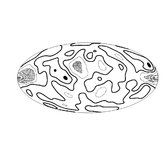
Figure 1: The COBE map 1 constructed using the combination method (see §3.1). The heavy lines show $0$, $1\sigma$ and $2\sigma$ (the interior of $2\sigma$ contours is shown in black); the light lines show $-1\sigma$ and $-2\sigma$ (the interior of $-2\sigma$ contours is shaded).

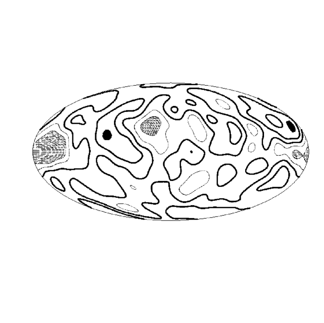
Figure 2: The COBE map 2 constructed using the subtraction method (see §3.1). The notations are same as in Fig. 1

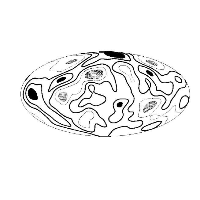
Figure 3: An example of a Gaussian map with the same as in COBE map 1 amplitudes $l(l+1)C_{l}/\sigma_{0}$

Figure 4: A region bounded by the level contours $\nu>\nu_{t}$ is shown. The closed polygons are the approximations to the boundaries based on the linear interpolation. Stars and circles are two sets of the inner boundary pixels corresponding to the boundaries. The dashed line shows a possible path on the grid connecting a pair of the inner boundary pixels that may belong to the same region or two different regions. If such a path intersects the both boundaries (i.e. the boundaries corresponding to the pixels in question) an even number of times then both pixels belong to the same (connected) region, otherwise they belong to different regions. In this case both numbers are zeros (i.e. even) and thus they belong to the same region.

Figure 5: The cumulative distribution functions of global Minkowski Functionals and the numbers of maxima/minima as a function of the temperature threshold (given in units of $\sigma$ for COBE map 1. Circles and triangles show the values for positive and negative thresholds respectively. The error bars corresponds one $\sigma$ dispersions calculated in 1000 Gaussian realizations.

Figure 6: Same as Fig. 5 but for the COBE map 2.

Figure 7: The cumulative distribution functions of partial Minkowski Functionals for both COBE maps. The shaded strips show $\pm\sigma$ regions for Gaussian realizations. Solid line shows the cumulative distribution functions for positive ($\nu>\nu_{t}$) and dashed line for negative ($\nu<\nu_{t}$) thresholds. Thick lines correspond to COBE map 1 and thin lines to COBE map 2. The threshold $\nu_{t}=2\sigma$.

Figure 8: Same as Fig. 7 with $\nu_{t}=1.5\sigma$.

Figure 9: Same as Fig .7 with $\nu_{t}=1\sigma$.

Figure 10: Same as Fig. 7 with $\nu_{t}=0.5\sigma$.

Figure 11: Same as Fig. 7 with $\nu_{t}=0$.

References

- Bandy et al (1996) Bandy, A.J., Górski, K.M., Bennett, C.L., Hinshaw, G., Kogut, A., & Smoot, G.F. 1996, ApJ, 468, L85
- Bennet et al. (1994) Bennett, C.L. et al., 1994, ApJ, 436, 423
- Bennet et al (1992) Bennett, C. L., et al. 1992, ApJ, 396, L7-L12
- Bernardeau (1997) Bernardeau, F. 1997, A&A, 324, 1
- Bond & Efstathiou (1987) Bond J.R., Efstathiou, G. 1987, MNRAS, 226, 655
- Bond & Jaffe (1998) Bond, J.R., Jaffe, A.H. 1998, astro-ph/9809043
- Brandenberger (1998) Brandenberger, R.H., 1998, astro-ph/9806473
- Coles (1988) Coles, P. 1988, MNRAS, 234, 509
- Colley et al (1996) Colley, W.N., Gott, III, J.R., & Park, C. 1996, MNRAS, 281, L82
- Doroshkevich (1970) Doroshkevich, A.G. 1970, Astrophysics, 6, 320
- Feldman et al (1994) Feldman, H.A., Kaiser, N. & Peacock, J. 1994, ApJ, 426 23–37
- Ferreira et al (1997) Ferreira, P.G., Magueijo, J., & Silk, J. 1997 Phys.Rev., D56, 7493
- Ferreira et al (1998) Ferreira, P.G., Magueijo, J., & Górski, K.M. 1998, ApJ, 503, L1
- Gott et al (1990) Gott, III, J.R., Melott, A.L., & Dickinson, M. 1986, ApJ, 306, 341
- Gott et al (1990) Gott, III, J.R., Park, C., Juskiewicz, R., Bies, W.E., Bennett, D.P., Bouchet, F.R., Stebins, A. 1990, ApJ, 352, 1
- Heavens (1998) Heavens, A.F. 1998, MNRAS, 299, 805
- Hadwiger (1957) Hadwiger, H. 1957, Vorlesungen über Inhalt, Oberfläche und Isoperimetre, Springer-Verlag, Berlin)
- Kendall & Stuart (1977) Kendall, M.G. & Stuart, A. 1977, , The Advanced Theory of Statistics, 4th edition, Charles Griffin.
- Knox et al (1998) Knox, L., Bond, J.R., Haffe, A.H., Segal, M., Charbonneau, D. 1998, Phys.Rev. D58, 083004
- Kogut et al (1996) Kogut, A., Bandy, A.J., Bennett, C.L., Górski, K.M., Hinshaw, G., Smoot, G.F., & Wright, E.L. 1996, ApJ, 464, L29
- Mecke, Buchert, & Wagner (1994) Mecke, K.R., Buchert, T, Wagner, H. 1994, A&A, 288, 697
- Melott et al (1989) Melott, A., Cohen, A., Hamilton, A., Gott, J., & Weinberg, D. 1989, ApJ345 618
- Minkowski (1903) Minkowski, H. 1903, Math. Ann., 57, 447
- Naselsky & Novikov (1995) Naselsky & Novikov 1995, ApJ, 444, L1
- Naselsky & Novikov (1998) Naselsky & Novikov 1998, ApJ, 507, 31
- Novikov & Jorgensen (1996) Novikov & Jorgensen 1996, ApJ471 521