Smoothed Particle Hydrodynamics in cosmology: a comparative study of implementations

Abstract

We analyse the performance of twelve different implementations of Smoothed Particle Hydrodynamics (SPH) using seven tests designed to isolate key hydrodynamic elements of cosmological simulations which are known to cause the SPH algorithm problems. In order, we consider a shock tube, spherical adiabatic collapse, cooling flow model, drag, a cosmological simulation, rotating cloud-collapse and disc stability. In the implementations special attention is given to the way in which force symmetry is enforced in the equations of motion. We study in detail how the hydrodynamics are affected by different implementations of the artificial viscosity including those with a shear-correction modification. We present an improved first-order smoothing-length update algorithm that is designed to remove instabilities that are present in the Hernquist and Katz [Hernquist & Katz 1989] algorithm. Gravity is calculated using the Adaptive Particle-Particle, Particle-Mesh algorithm.

For all tests we find that the artificial viscosity is the single most important factor distinguishing the results from the various implementations. The shock tube and adiabatic collapse problems show that the artificial viscosity used in the current hydra code performs relatively poorly for simulations involving strong shocks when compared to a more standard artificial viscosity. The shear-correction term is shown to reduce the shock-capturing ability of the algorithm and to lead to a spurious increase in angular momentum in the rotating cloud-collapse problem. For the disc stability test, the shear-corrected and current hydra artificial viscosities are shown to reduce outward angular momentum transport. The cosmological simulations produce comparatively similar results, with the fraction of gas in the hot and cold phases varying by less than 10% amongst the versions. Similarly, the drag test shows little systematic variation amongst versions. The cooling flow tests show that implementations using the force symmetrization of Thomas and Couchman [Thomas & Couchman 1992] are more prone to accelerate the overcooling instability of SPH, although the problem is generic to SPH. The second most important factor in code performance is the way force symmetry is achieved in the equation of motion. Most results favour a kernel symmetrization approach. The exact method by which SPH pressure forces are included in the equation of motion appears to have comparatively little effect on the results. Combining the equation of motion presented in Thomas and Couchman [Thomas & Couchman 1992] with a modification of the Monaghan and Gingold [Monaghan & Gingold 1983] artificial viscosity leads to an SPH scheme that is both fast and reliable.

1 Introduction

Smoothed Particle Hydrodynamics (SPH) [Gingold & Monaghan 1977, Lucy 1977] is a popular numerical technique for solving gas-dynamical equations. SPH is unique among numerical methods in that many algebraically equivalent – but formally different – equations of motion may be derived. In this paper we report the results of a comparison of several implementations of SPH in tests which model physical scenarios that occur in hierarchical clustering cosmology.

SPH is fundamentally Lagrangian and fits well with gravity solvers that use tree structures (Hernquist & Katz 1989, hereafter HK89) and mesh methods supplemented by short range forces (Evrard 1988; Couchman, Thomas & Pearce 1995, hereafter CTP95). In an adaptive form [Wood 1981], the algorithm lends itself readily to the wide range of densities encountered in cosmology, contrary to Eulerian methods which require the storage and evaluation of numerous sub-grids to achieve a similar dynamic range. SPH also exhibits less numerical diffusivity than comparable Eulerian techniques, and is much easier to implement in three dimensions, typically requiring 1000 or fewer lines of FORTRAN code.

The main drawback of SPH is its limited ability to follow steep density gradients and to correctly model shocks. Shock-capturing requires the introduction of an artificial viscosity [Monaghan & Gingold 1983]. A number of different alternatives may be chosen and it is not clear whether one method is to be preferred over another. The presence of shear in the flow further complicates this question.

Much emphasis has been placed upon the performance of SPH with a small number of particles (order 100 or fewer). Initial studies [Evrard 1988] of SPH on spherical cloud collapse indicated acceptable performance when compared to low resolution Eulerian simulations, with global properties, such as total thermal energy, being reproduced well. A more recent study (Steinmetz & Muller 1993, hereafter SM93), which compares SPH to modern Eulerian techniques (the Piecewise Parabolic Method [Collela & Woodward 1984], and Flux-Corrected-Transport methods) has shown that the performance of SPH is not as good as initially believed, and that accurate reproduction of local physical phenomena, such as the velocity field, requires as many as $10^{4}$ particles. In the context of cosmology with hierarchical structure formation, the small-$N$ performance remains critical as the first objects to form consist of tens – hundreds at most – of particles and form, by definition, at the limit of resolution. It is therefore of crucial importance to ascertain the performance of different SPH implementations in the small-$N$ regime. Awareness of this has caused a number of authors to perform detailed tests on the limits of SPH [Owens & Villumsen 1997, Bate & Burkert 1997]. To address these concerns, some of the tests we present here are specifically designed to highlight differences in performance for small $N$.

Our goal in this paper is to detail systematic trends in the results for different SPH implementations. Since these are most likely to be visible in the small-$N$ regime we concentrate on smaller simulations, using a larger number of particles to test for convergence. Because of the importance of the adaptive smoothing length in determining the local resolution we pay particular attention to the way in which it is calculated and updated. We are also concerned with the efficiency of the algorithm. Realistic hydrodynamic simulations of cosmological structure formation typically require $10^{4}$ or more time-steps. Therefore when choosing an implementation one must carefully weigh accuracy against computational efficiency. This is a guiding principle in our investigation.

The seven tests used in this study are:

• Sod shock (section 3.1)

• Spherical collapse (section 3.2)

• Cooling near density jumps(section 3.3)

• Drag on a cold clump(section 3.4)

• Hierarchical structure formation (section 3.5)

• Disc formation (section 3.6)

• Disc stability (section 3.7)

Each of these tests is described in the indicated section. The tests investigate various aspects of the SPH algorithm ranging from explicit tests of the hydrodynamics to investigations specific to cosmological contexts. The Sod shock (1978), although a relatively simple shock configuration, represents the minimum flow discontinuity that a hydrodynamic code should be able to reproduce. The spherical collapse test [Evrard 1988], although idealised, permits an assessment of the resolution necessary to approximate spherical collapse. It also allows a comparison with other authors’ results and with a high resolution spherically symmetric solution. The remaining tests are more closely tied to the arena of cosmological simulations. The cooling test looks at the problems associated with modelling different gas phases with SPH. A cold dense knot of particles embedded in a hot halo will tend to promote cooling of the hot gas because of the inability of SPH to separate the phases. The drag test looks at the behaviour of infalling satellites and the overmerging problem seen in SPH simulations [Frenk et al. 1996]. Finally, three tests consider the ability of the SPH algorithms to successfully model cosmic structure. First we look at the overall distribution of hot and cold gas in a hierarchical cosmological simulation, followed by an investigation of disc formation from the collapse of a rotating cloud (Navarro & White 1993), and the transport of angular momentum in discs. In each case we compare the different algorithms and assess the reliability of the SPH method in performing that aspect of cosmological structure formation.

The layout of the paper is as follows. Section 2 reviews the basic SPH framework that we use, including a description of the new approach developed to update the smoothing length. Next we examine the equations of motion and internal energy, and discuss the procedure for symmetrization of particle forces. In section 3 we present the test cases as listed above. Each of the subsections is self contained and contains a description and motivation for the test together with results and a summary comparing the relative merits of the different implementations together with an assessment of the success with which the SPH method can perform the test. Section 4 briefly summarises the main overall conclusions to be drawn from the test suite, indicating where each implementation has strengths and weaknesses and makes recommendations for the implementation which may be most useful in cosmological investigations.

During final prepartion of this paper, a preprint detailing a similar investigation was circulated by Lombardi et al.  [Lombardi et al. 1998].

2 Implementations of SPH

2.1 Features common to all implementations

All of the implementations use an adaptive particle-particle-particle-mesh (AP³M) gravity solver [Couchman 1991]. AP³M is more efficient than standard P³M, as high density regions, where the particle-particle summation dominates calculation time, are evaluated using a further P³M cycle calculated on a high resolution mesh. We denote the process of placing a high resolution mesh ‘refinement placing’ and the sub-meshes are termed ‘refinements’. The algorithm is highly efficient with the cycle time typically slowing by a factor of three under clustering. The most significant drawback of AP³M is that it does not yet allow multiple time-steps. However, the calculation speed of the global solution, compared with alternative methods such as the tree-code, more than outweighs this deficiency. Full details of the adaptive scheme, in particular accuracy and timing information, may be found in Couchman [Couchman 1991] and CTP95.

Time-stepping is performed using a Predict-Evaluate-Correct (PEC) scheme. This scheme is tested in detail against leapfrog and Runge-Kutta methods in CTP95. The value of the time-step, $dt$, is found by searching the particle lists to establish the Courant conditions of the acceleration, $dt_{a}$, and velocity arrays, $dt_{v}$. In this paper we introduce a further time-step criterion, $dt_{h}$, which prevents particles travelling too far within their smoothing radius, (see section 2.2). $dt$ is then calculated from $dt<\kappa\,\min(0.4dt_{v},0.25dt_{a},0.2dt_{h})$ where $\kappa$ is a normalisation constant that is taken equal to unity in adiabatic simulations. In simulations with cooling, large density contrasts can develop, and a smaller value of $\kappa$ is sometimes required. We do not have a Courant condition for cooling since we implement it assuming constant density (see below and CTP95 for further details).

SPH uses a ‘smoothing’ kernel to interpolate local hydrodynamic quantities from a sample of neighbouring points (particles). For a continuous system an estimate of a hydrodynamic scalar $A(\mn@boldsymbol{r})$ is given by,

$$\left<A(\mn@boldsymbol{r})\right>=\int d^{3}\mn@boldsymbol{r}^{\prime}A(\mn@boldsymbol{r}^{\prime})W(\mn@boldsymbol{r}-\mn@boldsymbol{r}^{\prime},h),$$ (1)

where $h$ is the ‘smoothing length’ which sets the maximum smoothing radius and $W(\mn@boldsymbol{r},h)$, the smoothing kernel, is a function of $|\mn@boldsymbol{r}|$. For a finite number of neighbour particles the approximation to this is,

$$\left<A(\mn@boldsymbol{r})\right>=\sum_{j}m_{j}{A(\mn@boldsymbol{r_{j}})\over\rho(\mn@boldsymbol{r}_{j})}\;W(\mn@boldsymbol{r}-\mn@boldsymbol{r}_{j},h),$$ (2)

where the radius of the smoothing kernel is set by $2h$ (for a kernel with compact support). The smoothing kernel used is the so-called $B_{2}$-spline [Monaghan & Lattanzio 1985],

$$W(\mn@boldsymbol{r},h)={W_{s}(r/h)\over h^{3}},$$ (3)

where if $x=r/h$,

$$W_{s}(x)={1\over 4\pi}\cases{4-6x^{2}+3x^{3},&$0\leq x\leq 1$;\cr(2-x)^{3},&$1<x\leq 2$;\cr 0,&$x>2$.}$$ (4)

The kernel gradient is modified to give a small repulsive force for close particles [Thomas & Couchman 1992],

$${dW_{s}(x)\over dx}=-{1\over 4\pi}\cases{4,&$0\leq x\leq 2/3$;\cr 3x(4-3x),&$2/3<x\leq 1$;\cr 3(2-x)^{2},&$1<x\leq 2$;\cr 0,&$x>2$.}$$ (5)

The primary reason for having a non-zero gradient at the origin is to avoid the artificial clustering noted by Schüssler & Schmidt [Schüssler & Schmidt 1981]. (Some secondary benefits are discussed by Steinmetz 1996.)

In standard SPH the value of the smoothing length, $h$, is a constant for all particles resulting in fixed spatial resolution. Fixed $h$ also leads to a slow-down in the calculation time when particles become clustered – successively more particles on average fall within a particle’s smoothing length. In the adaptive form of SPH [Wood 1981] the value of $h$ is varied so that all particles have a constant (or approximately constant) number of neighbours. This leads to a resolution scale dependent upon the local number density of particles. It also removes the slow-down in calculation time since the number of neighbours is held constant provided that the near neighbours can be found efficiently. In this work we attempt to smooth over 52 neighbour particles, and tests on the update algorithm we use (see section 2.2) show that this leads to a particle having between 30 and 80 neighbours, whilst the average remains close to 50.

A minimum value of $h$ is set by requiring that the SPH resolution not fall below that of the gravity solver. We define the gravitational resolution to be twice the S2 softening length [Hockney & Eastwood 1981], $\epsilon$, as at this radius the force is closely equivalent to the $1/r^{2}$ law. We quote the equivalent Plummer softening throughout the paper, as this is the most common force softening shape. Since the minimum resolution of the SPH kernel is the diameter of the smallest smoothing sphere, $4h_{min}$, equating this to the minimum gravitational resolution yields,

$$2\epsilon=4h_{min}.$$ (6)

Unlike other authors, once this minimum $h$ is reached by a particle, smoothing occurs over all neighbouring particles within a radius of $2h_{min}$. As a result setting a lower $h_{min}$ increases efficiency as fewer particles contribute to the sampling, but this leads to a mismatch between hydrodynamic and gravitational resolution scales which we argue is undesirable.

When required, radiative cooling is implemented in an integral form that assumes constant density over a time-step [Thomas & Couchman 1992]. The change in the specific energy, $e$, is evaluated from.

$$\int^{e-\Delta e}_{e}{de\over\Lambda}=-{n_{i}^{2}\over\rho_{i}}\Delta t,$$ (7)

where $\Delta t$ is the time-step, $n_{i}$ the number density and $n_{i}^{2}\Lambda$ is the power radiated per unit volume. In doing this we circumvent having a Courant condition for cooling, and hence it never limits the time-step.

2.2 An improved first-order smoothing-length update algorithm

Figure 1: Improvement in the neighbour counts as each component of the new algorithm is added. A rotating cloud collapse problem (see section 3.6) was repeated with each of our modifications to the HK89 algorithm. The improvement from the first panel (upper left) to the third panel (bottom left) is clear, the final panel shows a slight reduction in the range of neighbours and in the oscillation of the counts. The large increase in the maximum number of neighbours is due to the $h_{min}$ limit being reached. Time units are given in Gyr.

As stated earlier, in the adaptive implementation of SPH the smoothing length, $h$, is updated each time-step so that the number of neighbours is held close to, or exactly at, a constant. Ensuring an exactly constant number of neighbours is computationally expensive (requiring additional neighbour-list searching) and hence many researchers prefer to update $h$ using an algorithm that is closely linked to the local density of a particle.

We have used two guiding principles in the design of our new algorithm. First, since gravitational forces are attractive the algorithm will spend most of its time decreasing $h$ (void evolution is ‘undynamic’ and poses little problem to all algorithms). Second, smoothing over too many particles is generally preferable to smoothing over too few. Despite some loss of spatial resolution and computational efficiency, it does not ‘break’ the SPH algorithm. Smoothing over too few particles can lead to unphysical shocking.

A popular method for updating the smoothing length is to predict $h$ at the next time-step from an average of the current $h$ and the $h$ implied by the number of neighbours found at the current time-step (HK89). This is expressed as,

$$h_{i}^{n}={h_{i}^{n-1}\over 2}\left[1+\left({N_{s}\over N_{i}^{n-1}}\right)^{1/3}\right],$$ (8)

where $h_{i}^{n}$ is the smoothing length at time-step $n$ for particle $i$, $N_{s}$ is the desired number of neighbours and $N_{i}^{n-1}$ is the number of neighbours found at step $n-1$. The performance of this algorithm for a rotating cloud collapse problem (see section 3.6) is shown in the top left panel of Fig. 1. The rotating cloud collapse is a difficult problem for the $h$ update algorithm to follow since the geometry of the cloud rapidly changes from three to two dimensions. The plot shows that both the maximum and minimum number of neighbours (selected from all the SPH particles in the simulation) exhibit a significant amount of scatter. Clearly, the maximum number of neighbours increases rapidly once the $h=h_{min}$ limit is reached.

The rotating cloud problem demonstrates how this algorithm may become unstable when a particle approaches a high density region (the algorithm is quite stable where the density gradients are small). If the current $h$ is too large, the neighbour count will be too high leading to an underestimate of $h$. At the next step too few neighbours may be found. The result is an oscillation in the estimates of $h$ and in the number of neighbours as a particle accretes on to a high density region from a low density one. This oscillatory behaviour is visible in the fluctuations of the minimum number of neighbours in top left panel of Fig. 1.

The instability can be partially cured by using an extremely small time-step. However, this is not practical as simulations currently take thousands of time-steps. A solution suggested by Wadsley [Wadsley 1997] that helps alleviate the discontinuity in the number of neighbours, is to ‘count’ neighbours with a smoothed kernel rather than the usual tophat. This (normalised) weighted neighbour count is then used in the $h$ update equation rather than $N_{i}^{n-1}$. The instability in the standard HK89 algorithm is caused by the sharp discontinuity in the tophat at $r=2h$. Hence we require that the new kernel smoothly approach 0 at $2h$. Secondly, we wish to count the most local particles within the smoothing radius at full weight. Hence we consider a kernel that is unity to a certain radius followed by a smooth monotonic decrease to zero. We choose,

$$W_{nn}(r/h)=\cases{1,&$0\leq r/h<3/2$;\cr\pi W_{s}(4(r/h-3/2)),&$3/2\leq r/h\leq 2$,}$$ (9)

where $W_{s}(x)$ is the normalised $B_{2}$-spline kernel. We have experimented with changing the radius at which the counting kernel switches over to the spline, and a value of $r=3h/2$ has proven to be optimal, providing a good balance between the smoothness of the variation of the estimate and the closeness of actual number of neighbours to the desired number. At this value approximately half of the smoothing volume is counted at full weight. For smaller values the smoothed estimate becomes progressively more unreliable. Conversely as the limiting radius is increased the gradient of the kernel at $r\simeq 2h$ becomes too steep. The improvement in fluctuation of the maximum and minimum number of neighbours can be seen in the top right panel of Fig. 1.

The next step in the construction of the new algorithm is to adjust the the average used to update $h$. The primary reason for doing this is to avoid sudden changes in the smoothing length. Whilst the neighbour counting kernel helps to alleviate this problem, it does not remove it entirely. Secondly, since we shall limit the time-step by only allowing the particles to move a certain fraction of $h$ it is also useful to limit the change in $h$. The motivation here is that a particle which is approaching a high density region, for example, and is restricted to move $0.2h$ per time-step should only be allowed to have $h\rightarrow 0.9h$ (since the smoothing radius is $2h$). However, a particle at the centre of homologous flow must be able to update faster since collapse occurs from all directions. To account for this it is helpful to permit a slightly larger change in $h$, $h\rightarrow 0.8h$ for example.

Setting $s=(N_{s}/N_{i}^{n-1})^{1/3}$, we may express equation 8 as

$$h_{i}^{n}=h_{i}^{n-1}(1-a+as),$$ (10)

where $a$ is a weighting coefficient, and for equation 8, $a=0.5$. We have tested the performance of this average for $a\in[0.2,0.5]$. A value of $a=0.4$ proved optimal, reducing scatter significantly yet allowing a sufficiently large change in $h$. A problem remains that if $s\simeq 0$ then $h_{i}^{n}=0.6h_{i}^{n-1}$, which represents a large change if one limits the time-step according to an $h/v$ criterion. Hence we have implemented a scheme that has the asymptotic property $h_{i}^{n}=0.8h_{i}^{n-1}$, but for small changes in $h$ it yields $h_{i}^{n}=h_{i}^{n-1}(0.6+0.4s)$. The function we use for determining the weighting variable $a$ is,

$$a=\cases{0.2(1+s^{2}),&$s<1$;\cr 0.2(1+1/s^{3}),&$s\geq 1$.}$$ (11)

A plot of this function compared to the 0.6,0.4 weighted average can be seen in Fig. 2. The lower left panel of Fig. 1 shows that introduction of this average reduces the scatter in both the maximum and minimum number of neighbours.

Even with the improvements made so far it remains possible that the particle may move very quickly on to a high density region causing a sudden change that cannot be captured by the neighbour counting kernel. Thus it is sensible to limit the time-step according to a ‘Courant condition’ which is the smoothing radius divided by the highest velocity within the smoothing radius. Further, the velocity $\mn@boldsymbol{v}_{r}$, must be measured within the frame of the particle under consideration, $\mn@boldsymbol{v}_{r}=\mn@boldsymbol{v}_{i}-\mn@boldsymbol{v}_{j}$. The new time-step criterion may be summarised,

$$dt=C_{h}\min_{i}(h_{i}/\max_{j}(|\mn@boldsymbol{v}_{i}-\mn@boldsymbol{v}_{j}|),$$ (12)

where $C_{h}$ is the Courant number and the $i,j$ subscripts denote a reduction over the variable indicated. We have chosen $C_{h}=0.2$, which is usually the limiting factor in time-step selection. The gains in introducing this condition are marginal for the neighbour count in this test (maximum and minimum values are within a tighter range and show slightly less oscillation).

When taken together all of these adjustments combine to make a scheme that is both fast and very stable. The final result of including these improvements is seen in the lower right hand panel of Fig. 1.

Figure 2: Weighting function compared to simple weighted averages.

2.3 Equations of motion

The SPH equation of motion is derived from,

$${dv\over dt}=-{1\over\rho}\nabla P,$$ (13)

using identities involving the pressure and density. An excellent review of this derivation, and why so many different schemes are possible, may be found in Monaghan [Monaghan 1992]. In short, different identities produce different equations of motion and a clear demonstration of this can be seen by comparing the equations of motion of HK89 to those of SM93.

Once an adaptive scheme is implemented in SPH, neighbour smoothing develops a dualism – the smoothing may be interpreted as either a “gather” or a “scatter” process. If we attempt to smooth a field at the position of particle $i$, then the contribution of particle $j$ to the smoothed estimate may be evaluated using the value of $h$ from either particle $i$ (gather) or particle $j$ (scatter). For constant $h$ SPH the schemes are equivalent.

The uncertainty in the neighbour smoothing may be circumvented by using a formalism based upon the average of the two smoothing lengths [Evrard 1988, Benz 1990]. Under this prescription, the gather and scatter interpretations are equivalent since the smoothing length for particles $i$ and $j$ are the same. We call this prescription $h$-averaging. The density estimate under this prescription is given by,

$$\left<\rho(\mn@boldsymbol{\mn@boldsymbol{r}_{i}})\right>=\sum_{j=1}^{N}m_{j}W(\mn@boldsymbol{r}_{i}-\mn@boldsymbol{r}_{j},h_{ij}),$$ (14)

where,

$$h_{ij}=(h_{i}+h_{j})/2,$$ (15)

and the neighbour search is conducted over particles for which $r_{ij}<2h_{ij}$.

Most $h$-averaging schemes use the arithmetic mean of the smoothing lengths but it is possible to consider other averages (any ‘average’ that is symmetric in $i-j$ is potentially acceptable). Two other averages of interest are the geometric mean and the harmonic mean. Note that the harmonic and geometric means both pass through the origin where as the arithmetic mean does not. This has potentially important consequences when particles with large $h$ interact with particles that have a small $h$. This situation occurs at the boundary of high density regions in simulations with radiative cooling (see section 3.3 for a detailed discussion of this).

An alternative way of circumventing the smoothing uncertainty (HK89) is to combine the “gather” and “scatter” interpretations into one hybrid framework by averaging the kernels. In this scheme the density estimate is given by,

$$\left<\rho(\mn@boldsymbol{r}_{i})\right>=\sum_{j=1}^{N}m_{j}[W(\mn@boldsymbol{r}_{i}-\mn@boldsymbol{r}_{j},h_{i})+W(\mn@boldsymbol{r}_{i}-\mn@boldsymbol{r}_{j},h_{j})]/2,$$ (16)

and we denote this scheme kernel averaging. The averaged kernel then replaces the normal kernel in all equations. Rewriting equation 13 using the identity,

$${\nabla P\over\rho}=\nabla{P\over\rho}+{P\over\rho^{2}}\nabla\rho,$$ (17)

the SPH equation of motion with kernel averaging becomes,

$${d\mn@boldsymbol{v}_{i}\over dt}=-\sum_{j=1}^{N}m_{j}\left({P_{i}\over\rho_{i}^{2}}+{P_{j}\over\rho_{j}^{2}}\right)\times$$

$$\;\;\;\;\;\;\;\;\;\;\nabla_{i}[W(\mn@boldsymbol{r}_{i}-\mn@boldsymbol{r}_{j},h_{i})+W(\mn@boldsymbol{r}_{i}-\mn@boldsymbol{r}_{j},h_{j})]/2.$$ (18)

This equation of motion is used in SM93.

Thomas & Couchman (1992, hereafter TC92), present an alternative prescription where the force term is symmetrized and the density is calculated under the gather interpretation. Using the standard pressure and density identity in equation 17, the acceleration for particle $i$ is written,

$${d\mn@boldsymbol{v}_{i}\over dt}=\sum_{j=1}^{N}{\mn@boldsymbol{f}_{ij}\over m_{i}}=-\sum_{j=1}^{N}m_{j}{P_{i}\over\rho_{i}^{2}}\nabla_{i}W(\mn@boldsymbol{r}_{i}-\mn@boldsymbol{r}_{j},h_{i})$$

$$\;\;\;\;\;\;\;\;\;\;\;\;\;\;\;\;\;\;\;\;\;\;\;\;+\sum_{j=1}^{N}m_{j}{P_{j}\over\rho_{j}^{2}}\nabla_{j}W(\mn@boldsymbol{r}_{i}-\mn@boldsymbol{r}_{j},h_{j}).$$ (19)

This symmetrization is used in the current implementation of the publically available code, hydra. When combined with an artificial viscosity that does not require the pre-computation of all density values this scheme is extremely efficient.

In deriving equation 19 the approximation,

$$\nabla_{i}W(\mn@boldsymbol{r}_{i}-\mn@boldsymbol{r}_{j},h_{i})\simeq-\nabla_{j}W(\mn@boldsymbol{r}_{i}-\mn@boldsymbol{r}_{j},h_{j})$$ (20)

was used. This approach to symmetrization of the equation of motion is fundamentally different to the other two schemes which both result in a kernel symmetric in $i$ and $j$. The approximation is not correct to first order in $h$ and may introduce small errors. If this symmetrization is supplemented by either $h$-averaging or kernel averaging (there is no argument against this) then the substitution is correct to first order in $h$ (but not in $\nabla h$).

When SPH is implemented in its adaptive form equation 18 will not guarantee conservation of momentum. To do so one must alter the neighbour list so that for any particle $i$ which smooths over particle $j$ the converse is also true. This will not necessarily be true if one smooths over the nearest 52 neighbours for each particle. Note that equation 19 does conserve momentum regardless of the neighbour list used.

In the SPH–AP³M solver an SPH particle only has gas forces evaluated within a refinement if it has a sufficiently small $h$ (see CTP95 for a detailed discussion of this topic). The introduction of $h$-averaging complicates refinement loading since a particle no longer has a well defined $h$ (one must consider all $h_{ij}$ values). To establish which particles are to be evaluated, one must calculate all the $h_{ij}$ values for a particle, which is computationally costly. As a compromise, we place particles in a refinement only if $1.4\times 2h$ is smaller than the sub-mesh search length (note that for arithmetic $h$-averaging a search to $2\times 2h$ will ensure that all neighbours are found and we use this search radius in sections 3.5, 3.6 & 3.7). This does not absolutely guarantee that all the neighbour data for a particle will be placed in the refinement data arrays but we have found no detectable difference between this method and the full $h_{ij}$ method.

2.4 Internal energy equation

The SPH internal energy equation is derived from,

$${du\over dt}=-{P\over\rho}\nabla.\mn@boldsymbol{v}.$$ (21)

The SPH estimate for $\nabla.\mn@boldsymbol{v}$ may be used to calculate $du/dt$ directly, yielding the internal energy equation for particle $i$,

$${d\epsilon_{i}\over dt}=-{P_{i}\over\rho_{i}}\nabla.\mn@boldsymbol{v}_{i}.$$ (22)

Explicitly writing the summation for the SPH estimate gives,

$${d\epsilon_{i}\over dt}=\sum_{j}m_{j}{P_{i}\over\rho^{2}_{i}}(\mn@boldsymbol{v}_{i}-\mn@boldsymbol{v}_{j}).\nabla_{i}W(\mn@boldsymbol{r}_{i}-\mn@boldsymbol{r}_{j},h).$$ (23)

Substituting $h=h_{ij}$ and inserting the artificial viscosity $P_{i}\rightarrow P_{i}+\rho_{i}^{2}\Pi_{ij}/2$ (see equation 26), yields the internal energy equation used in SM93. Whilst not strictly compatible with equation 18 (equation 23 has no dependence upon $P_{j}$) it can nevertheless be shown that energy will be conserved [Benz 1990].

An internal energy equation may be constructed using the same symmetrization as equation 19, yielding,

$${d\epsilon_{i}\over dt}={1\over 2}\sum_{j=1}^{N}m_{j}(\mn@boldsymbol{v}_{i}-\mn@boldsymbol{v}_{j}).{P_{i}\over\rho_{i}^{2}}\nabla_{i}W(\mn@boldsymbol{r}_{i}-\mn@boldsymbol{r}_{j},h_{i})$$

$$\;\;\;\;\;\;\;\;\;\;\;-{1\over 2}\sum_{j=1}^{N}m_{j}(\mn@boldsymbol{v}_{i}-\mn@boldsymbol{v}_{j}).{P_{j}\over\rho_{j}^{2}}\nabla_{j}W(\mn@boldsymbol{r}_{i}-\mn@boldsymbol{r}_{j},h_{j}).$$ (24)

A similar equation was considered in TC92, and was shown to exhibit excellent energy conservation. In CTP95 the entropy scatter produced by this equation was compared to that of equation 22 and was shown to be significantly larger. Therefore to avoid this problem we only consider the energy equation 22.

It has been shown by Nelson & Papaloizou (1993,1994) and Serna, Alimi & Chieze [Serna et al. 1996], that inclusion of the $\nabla h$ terms, in both the equation of motion and internal energy, is necessary to ensure conservation of both energy and entropy. We chose to neglect these terms due to the overhead involved in computing them.

2.5 Artificial viscosity algorithms

An artificial viscosity is necessary in SPH to dissipate convergent motion and hence prevent interpenetration of gas clouds [Monaghan & Gingold 1983].

We investigate four different types of artificial viscosity. The first considered is the implementation of TC92, where an additional component is added to a particle’s pressure,

$$P_{i}\rightarrow\cases{P_{i}+\rho_{i}[-\alpha c_{i}h_{i}\nabla.\mn@boldsymbol{v}_{i}+\beta(h_{i}\nabla.\mn@boldsymbol{v}_{i})^{2}],&$\nabla.\mn@boldsymbol{v}_{i}<0$;\cr P_{i},&$\nabla.\mn@boldsymbol{v}_{i}\geq 0$,}$$ (25)

where $c_{i}$ is the sound speed for the particle. Typically, the viscosity coefficients are $\alpha=1$ and $\beta=2$. This algorithm is a combination of the Von Neumann-Richtmeyer and bulk viscosity prescriptions (see Gingold & Monaghan 1983). A notable feature is that it uses a $\nabla.\mn@boldsymbol{v_{i}}$ ‘trigger’ so that it only applies to particles for which the local velocity field is convergent. This is different from most other implementations, which use an $\mn@boldsymbol{r}_{ij}.\mn@boldsymbol{v}_{ij}<0$ trigger. With this artificial viscosity the first term in equation 19 does not depend upon the density of particle $j$. This is advantageous numerically since it is not necessary to construct the neighbour lists twice. In this circumstance one can reduce the SPH search over particles to a primary loop, during which the density is calculated and the neighbour list is formed and stored, followed by a secondary loop through the stored neighbour list to calculate the forces and internal energy.

A modification of this artificial viscosity prescription is to estimate the velocity divergence over a smaller number of neighbours found by searching to a reduced radius. This was motivated by the observation that in some circumstances the gas does not shock as effectively as when a pairwise viscosity is employed. The reduced search radius leads to a higher resolution (but likely noisier) estimate of $\nabla.\mn@boldsymbol{v}$.

The third artificial viscosity we consider is the standard ‘Monaghan’ artificial viscosity [Monaghan & Gingold 1983]. This artificial viscosity has an explicit $i-j$ particle label symmetry which is motivated to fit with equation 18. In this algorithm the summation of $P/\rho^{2}$ terms in equation 18 is extended to include a term $\Pi_{ij}$, which is given by,

$$\Pi_{ij}={-\alpha\mu_{ij}\bar{c}_{ij}+\beta\mu_{ij}^{2}\over\bar{\rho}_{ij}},$$ (26)

where,

$$\mu_{ij}=\cases{\bar{h}_{ij}\mn@boldsymbol{v}_{ij}.\mn@boldsymbol{r}_{ij}/(r_{ij}^{2}+\nu^{2}),&$\mn@boldsymbol{v}_{ij}.\mn@boldsymbol{r}_{ij}<0$;\cr 0,&$\mn@boldsymbol{v}_{ij}.\mn@boldsymbol{r}_{ij}\geq 0$,}$$ (27)

where the bar denotes arithmetic averaging of the quantities for particles $i$ and $j$ and $\nu^{2}=0.01\bar{h}_{ij}^{2}$ is a term included to prevent numerical divergences. Again, typical values for the coefficients are $\alpha=1$ and $\beta=2$ although for problems involving weak shocks values of 0.5 and 1, respectively, may be preferable. This artificial viscosity has the same functional dependence upon $h$ as the $\nabla.\mn@boldsymbol{v}$ version. Since this algorithm utilises a pairwise evaluation of the relative convergence of particles it is capable of preventing interpenetration very effectively. A drawback is that it requires the neighbour list for particles to be calculated twice since the force on particle $i$ depends explicitly on the density of particle $j$ (storing all the neighbour lists is possible, but in practice too memory consuming).

One major concern about this algorithm relates to its damping effect on angular momentum. In the presence of shear flows, $\nabla.\mn@boldsymbol{v}=0$, $\nabla\times\mn@boldsymbol{v}>0$ the pairwise $\mn@boldsymbol{r}_{ij}.\mn@boldsymbol{v}_{ij}$ term can be non zero and hence the viscosity does not vanish. This leads to a large shear viscosity which is highly undesirable in simulations of disc formation, for example. A way around this problem is to add a shear-correcting term to the artificial viscosity [Balsara 1995]. The modification we consider is given by Steinmetz (1996);

$$\Pi_{ij}\rightarrow\tilde{\Pi}_{ij}=\Pi_{ij}\bar{f}_{ij},$$ (28)

where,

$$\bar{f}_{ij}={f_{i}+f_{j}\over 2},$$ (29)

and,

$$f_{i}={|\left<\nabla.\mn@boldsymbol{v}\right>_{i}|\over|\left<\nabla.\mn@boldsymbol{v}\right>_{i}|+|\left<\nabla\times\mn@boldsymbol{v}\right>_{i}|+0.0001c_{i}/h_{i}}.$$ (30)

For pure compressional flows $f=1$ and the contribution of $\Pi_{ij}$ is unaffected whilst in shear flows $f=0$ and the viscosity is zero. This modification has been studied by Navarro & Steinmetz [Navarro & Steinmetz 1997] who found that the dissipation of angular momentum is drastically reduced in small-$N$ problems using this method. However, of concern is whether this modification leads to poorer shock-capturing. This may arise due to sampling error in the SPH estimates of the velocity divergence and curl. We compare schemes using the shear-corrected viscosity against the standard Monaghan viscosity.

The efficiency gained from having an artificial viscosity that does not depend upon the density of particle $j$ has motivated us to consider the following modification of the Monaghan viscosity: we use the same quantities as equation 26, except that,

$$\bar{\rho}_{ij}\rightarrow\tilde{\rho}_{ij}=\rho_{i}(1+(h_{i}/h_{j})^{3})/2,$$ (31)

which provides an estimate of $\bar{\rho}_{ij}$. The estimate is based upon the approximation $\rho_{j}\simeq\rho_{i}h_{i}^{3}/h_{j}^{3}$. We have plotted this estimate against the real $\rho_{j}$ in the spherical collapse test (see section 3.2) and find the maximum error to be a factor of ten. In practice the maximum error is dependent upon the problem being studied, but in general we have found the error to usually fall in the range of a factor of two. Note that the shear-free single-sided Monaghan variant would have to implemented as,

$$\tilde{\Pi}_{ij}={-\alpha\mu_{ij}\bar{c}_{ij}+\beta\mu_{ij}^{2}\over\tilde{\rho}_{ij}}f_{i},$$ (32)

thereby removing the $j$ index. Despite the estimated quantity $\tilde{\rho}_{ij}$, this artificial viscosity, when used in conjunction with the equation of motion in equation 19, still results in a momentum-conserving scheme.

In principle the $\nabla.\mn@boldsymbol{v}$-based artificial viscosity should not suffer the problem of damping during pure shear flows, since the artificial viscosity only acts in compressive flows. A useful test is to supplement this artificial viscosity with the shear-correction term. This enables an estimate to be made of the extent to which the correction term under-damps due to SPH sampling errors.

3 Test scenarios

Version	Artificial Viscosity	symmetrization	equation of motion
1	TC92	TC92	TC92
2	TC92+shear correction	TC92	TC92
3	local TC92	TC92	TC92
4	Monaghan	arithmetic $h_{ij}$	SM93
5	Monaghan	harmonic $h_{ij}$	SM93
6	Monaghan	kernel averaging	SM93
7	Monaghan+shear correction	arithmetic $h_{ij}$	SM93
8	Monaghan+shear correction	harmonic $h_{ij}$	SM93
9	Monaghan+shear correction	kernel averaging	SM93
10	Monaghan	TC92	TC92
11	Monaghan $\tilde{\rho}_{ij}$	TC92	TC92
12	Monaghan $\tilde{\rho}_{ij}$	TC92 + kernel av	TC92

Table 1: Summary of the implementations examined. ‘Monaghan’ is the artificial viscosity of equation 26. Steinmetz-type shear correction Steinmetz (1996) is applied where noted. The remaining terms are discussed in the text.

The SPH implementations that we examine are listed in Table 1. The list, whilst not exhaustive, represents a range of common variants for the SPH algorithm. Our motivation is to determine the extent to which the different implementations affect behaviour in cosmological settings. In all cases we employ the full $h$-updating scheme described in section 2.2.

We have chosen twelve different combinations of artificial viscosity, symmetrization and equation of motion. The first is that employed by the hydra code, (Couchman, Pearce & Thomas 1996). We then add a shear correction term to this and also try a localised artificial viscosity (as discussed in section 2.5), resulting in three versions close to the TC92 formalism. We then have three versions based on the popular Monaghan viscosity (again see section 2.5) each with and without shear correction. These employ different $h$-averaging schemes or kernel averaging as discussed in section 2.3 and are the most common schemes found in the literature. Finally we have three new schemes which attempt to combine the best features of the other implementations.

3.1 Shock tube

The shock tube is an environment which provides an abundant source of simple tests fundamental to hydrodynamical simulations. One well-studied test [Monaghan & Gingold 1983, Hernquist & Katz 1989, Rasio & Shapiro 1991] is the Sod shock [Sod 1978] for which analytical solutions are given by Hawley, Smarr & Wilson [Hawley et al. 1984] and Rasio & Shapiro [Rasio & Shapiro 1991]. In this test two regions of uniform but different density gas are instantaneously brought into contact. If initially high density and pressure gas is to the left and the low density and pressure gas is to the right then a rarefaction wave will propagate left into the high density gas whilst a shock wave will propagate rightwards into the low density gas. Between these there will be a contact discontinuity where the pressure is continuous but the density jumps. This behaviour is shown in Fig. 3 where the analytic solution is superimposed on the simulation results.

Many authors have carried out this test in 1-dimension, but this is of limited use as most interesting astrophysical phenomena are 3-dimensional. The 1-dimensional results do not automatically carry over to 3-dimensions. The core of the SPH approach – the smoothing kernel – must be altered to take account of the different volume elements. Otherwise far too much emphasis will be placed on the central region in the 1-dimensional tests. Additionally, in 1-dimension, interpenetration is reduced.

Rasio & Shapiro (1991) perform this test in 3-dimensions and note the large increase in numerical scatter and interpenetration this produces. This is partly because of their choice of initially randomly distributed particles which introduces large fluctuations in the supposedly uniform initial density and pressure. Contrary to their assertion, this is not a particle distribution encountered in the course of a typical SPH simulation. SPH is adept at equalising density and pressure differences and rapidly relaxes from such an initial state.

3.1.1 Initial conditions

We have altered our standard cubical simulation volume to match the geometry of a shock tube. The tube has an aspect ratio of 16 and all the boundaries are periodic. We take the high density gas to have $\rho_{l}=4$ and $p_{r}=1$. The low density gas has $\rho_{r}=1$ and $p_{r}=0.1795$. In accordance with the rest of our tests we set $\gamma={5\over 3}$.

In this test there are 4096 low density particles and 16384 high density particles. Before starting the test itself each of the regions is independently evolved at constant temperature until induced random fluctuations have damped away. This reduces the spurious initial fluctuations mentioned above and closely mimics the conditions typical of a cold flow in an SPH simulation.

Note that even if the particles resided in exactly the correct positions to produce the theoretical curve, it is impossible to reproduce the discontinuities due to the inherent smoothing in SPH estimates. The smoothed theoretical curves are shown in Fig. 3.

Figure 3: A comparison between the analytic result (solid abrupt line) and those from version 1 (dashed line) and version 12 (solid line). Also shown is the ideal result (dotted line) obtained by smoothing the theoretical result with the SPH kernel. Codes 2 and 3 match the profile of 1 closely, the remainder match that of 12. The x-axis is in units of the SPH smoothing length, $h$, in the low density gas and the zero point is the original interface between the high- and low-density gas. The top-left panel shows a zoom into the right-moving shock, the area where the largest difference between the codes is seen.

3.1.2 Shock evolution and results

For all versions only around 35 time-steps are required to reach the state shown in Fig. 3, by which time the shock front and the front of the rarefaction wave have moved around $10h_{low}$. The asymptotic solutions are recovered around each of the density jumps and even the small drop in entropy at the shock front is well modelled. Although the correct jump conditions are captured for the rarefaction wave and none of the versions introduces spurious entropy, the density gradient is too shallow. This effect has also been seen previously [Rasio & Shapiro 1991, CTP95]. At the contact discontinuity the entropy jump is overshot by all the codes, with the problem worse for versions 1–3. The blip in the ideally uniform pressure at this point is due to the SPH smoothing of the discontinuous density [Monaghan & Gingold 1983]. The top-left panel of Fig. 3 shows that the right-moving shock front in versions 1–3 is broadened over a region about twice that seen for versions 4–12 which themselves have about twice the width of the smoothed theoretical solution.

Figure 4: The scatter in velocity perpendicular to the shock tube for versions 1, 7 & 12. The x-axis is in units of the SPH search length in the low density gas. All the particles in the region of interest are shown as single points. The scatter is much higher and the profile is clearly different for version 1 than for either of the other versions. Version 12 exhibits notably less post-shock ringing than 7. Of the other codes, Versions 2 and 3 look like version 1, versions 8 and 9 look like version 7 and versions 4, 5, 6, 10 and 11 look like version 12.

3.1.3 Particle interpenetration

We have also used this test to study the level of flow interpenetration. Ideally there should be no interpenetration and the flow should remain smooth with the particles in well defined slabs at the end. As Fig. 4 shows for versions 1, 2 and 3 the flow is far from smooth, with large differences in velocity at any one point along the shock tube. Versions 7, 8 and 9 show much less scatter but produce noticeable post-shock oscillation whilst the remaining versions all produce a very smooth flow with little velocity scatter. Due to the large intrinsic scatter, versions 1–3 of the code suffer from much greater interpenetration than the other versions. These effects are exacerbated in the presence of some initial turbulence. The locally averaged nature of the viscosity employed by versions 1–3 allows regions to interpenetrate. The shear-corrected versions (7–9), despite producing just as sharp a density jump as the remaining versions, also perform poorly in the interpenetration test because interpenetrating streams of particles can mimic shear.

3.1.4 Summary

For this test the versions split into 2 main groups with the more accurate codes (4–12) further sub-dividing into two groups depending upon whether or not the viscosity is shear corrected. Versions 1–3 produce broader shocks and suffer from greater interpenetration because these codes employ a locally averaged method for calculating the viscosity. All the other versions employ a particle-particle approach to the viscosity calculation and hence resolve shorter scales. The addition of a shear-correction term to prevent transport of angular momentum degrades the performance of these codes for this particular test. Although the shock profiles are very similar (see Fig. 3) they produce a flow which is less smooth (see Fig. 4) and suffers from greater interpenetration than versions 4, 5, 6, 10, 11 and 12.

3.2 Collapse of a spherical cloud

Figure 5: Convergence of energy values with particle number for the Evrard collapse test using version 12. Energy is plotted on the y axis and time along the x axis in normalised units. The sets of curves are, from top to bottom, the thermal, kinetic, total and potential energies. There is comparatively little difference between the 4776 and 485 particle collapse because they were run with the same softening length. The 30796 particle run matches the solution calculated in SM93 very accurately.

This test examines the adiabatic collapse of an initially isothermal spherical gas cloud. We denote this test the ‘Evrard collapse’ since it first appears in Evrard (1988), and since then has proved itself as a useful test case for combined SPH-gravity codes (e.g. HK89, SM93, Serna et al. 1996, Hultman & Kallander 1997).

3.2.1 Units and initial conditions

Test results are presented in normalised units. The density, internal energy, velocity, pressure and time are normalised by $3M/4\pi R^{3}$, $GM/R$, $(GM/R)^{1\over 2}$, $\rho u$ and $(R^{3}/GM)^{1\over 2}$, respectively, where $R$ denotes the initial radius and $M$ the total mass. The initial physical density distribution is given by,

$$\rho(r)={M(R)\over 2\pi R^{2}}{1\over r},$$ (33)

which is achieved by applying a radial stretch to an initially uniform grid [Evrard 1988]. We prefer this configuration over a random one since it has significantly less sampling error than a random distribution [Hultman & Kallander 1997]. The internal energy of the system is chosen to be 0.05$GM/R$, and the adiabatic index $\gamma=5/3$. The softening length used for each simulation is given in the caption to Table 2.

3.2.2 System evolution

The evolution of the system is shown in Fig. 5. As the collapse occurs the gas is heated until the temperature of the core rises sufficiently to cause a ‘bounce’, after which a shock propagates outward through the gas. After the shock has passed through the majority of the gas, the final state of the system is one of virial equilibrium. Along with placing emphasis on the performance of the implementations for small-$N$ systems we also study convergence at larger values of $N$. A summary of the runs performed is presented in Table 2.

Figure 6: Radial profiles for the 30976 and 485 particle collapses at t=0.8 are displayed in the left and right hand columns respectively. For the 30976 particle tests the density, pressure and velocity are plotted using Lagrangian bins of size $4\times 52=208$ particles, corresponding to $4\,N_{smooth}$ and for the 485 particle collapses a single line connects all particles. Error bars on the 30976 particle plots show the maximum variation within bins. The velocity plots are displaced by intervals of -0.2 vertically for easier interpretation. Notably versions 1 and 3 show significant differences to versions 4, 7 and 12, in particular both the density and pressure are underestimated (as compared to the solution calculated in SM93). Version 3 shows a better capture of the collapsing shock front than version 1, this effect being most evident in the pressure plot. Versions 4, 7 and 12 show excellent agreement, being difficult to distinguish at all radii. Version 7 shows that the inclusion of the shear-free term has little effect on the radial profile.

Table 2: Results of Evrard collapse test.

Version	$N_{steps}$	$\Delta E/E(\times 10^{-3})$	$\Delta L(\times 10^{-7})$	$N_{par}$
1	62	$6.2$	$49$	485
2	62	$3.3$	$31$	485
3	66	$1.1$	$38$	485
4	94	$2.5$	$11$	485
5	88	$1.0$	$39$	485
6	129	$1.7$	$23$	485
7	104	$0.8$	$15$	485
8	95	$0.8$	$65$	485
9	135	$1.2$	$28$	485
10	90	$1.5$	$62$	485
11	84	$1.5$	$40$	485
12	103	$0.6$	$29$	485
1	82	$6.1$	$2.8$	4776
2	101	$6.1$	$6.7$	4776
3	98	$1.9$	$14$	4776
4	240	$3.1$	$45$	4776
5	241	$3.2$	$24$	4776
6	231	$3.5$	$63$	4776
7	243	$3.2$	$68$	4776
8	252	$3.1$	$38$	4776
9	242	$3.7$	$64$	4776
10	234	$2.9$	$27$	4776
11	227	$2.8$	$29$	4776
12	241	$2.8$	$7.0$	4776
1	289	$0.3$	$1.3$	30976
3	218	$1.9$	$0.91$	30976
4	418	$4.4$	$1.4$	30976
6	411	$4.5$	$5.5$	30976
11	405	$3.6$	$7.0$	30976
12	489	$4.7$	$2.9$	30976

Values for the 485 particle test are given at t=4.3, for the 4776 test at t=3.4 and for the 30976 test at t=2.0. $\Delta L$ is measured in internal code units, normalising by $L_{start}$ is not possible since $L_{start}=0$. The 485 and 4776 particle tests used a softening length of 0.05R, the 30976 particle tests used a softening length of 0.02R.

3.2.3 Results from the 485 particle collapse

With the $N$ considered here, the standard hydra code, and variants of it, do relatively poorly in this test. A lack of thermalization is clearly visible in Fig. 8, where the difference in energy between versions 1–3 of the code and version 12 are shown along the top row. These implementations all have thermal energy peaks that are half that of the other codes. The other versions perform reasonably similarly with minor differences being seen in the peak thermal energy and in the strength of post bounce oscillation (note the change in $y$-axis scale on the bottom two rows of Fig. 8).

Figure 7: Thermal energy plot for the 485 particle collapse, comparing versions 1, 3, 7 and 12. A lower peak thermalization is clearly visible in versions 1 and 3, whilst 7 and 12 show similar profiles. A comparative plot of the energy difference between version 12 and the other codes is shown in Fig. 8.

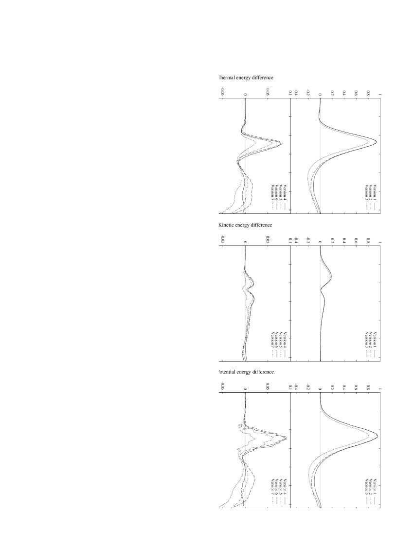
Figure 8:

Figure 9:

The modified viscosity variant, 3, is slightly better at thermalization than versions 1 & 2 but still much worse than any of the other versions. This indicates that the artificial viscosity is the primary factor in deciding the amount of kinetic energy that is thermalised (as expected). The more local estimate of $\nabla.\mn@boldsymbol{v}$ used in version 3 captures the strong flow convergence near the bounce better than the standard estimate, leading to greater dissipation. At the other extreme the pairwise Monaghan viscosity, which uses the $\mn@boldsymbol{r}.\mn@boldsymbol{v}$ trigger, leads to far more dissipation at bounce. It is important to note that the final energy values for the virialised state are very similar for all codes, even though their evolution is very different in some cases.

Similar characteristics can be seen in the kinetic energy graphs. The gas in versions 1–3 develops very little kinetic energy. The primary cause of this is the $\nabla.\mn@boldsymbol{v}$ artificial viscosity which trips during the early stages of collapse (prior to t=0.6) and causes an increase in the thermal energy for all particles. This acts to decrease the compressibility of the gas. For all the other codes which use the Monaghan viscosity (or variant), the $\mn@boldsymbol{r}.\mn@boldsymbol{v}$ trigger produces far less dissipation during the early stages of evolution, and the gas develops more kinetic energy.

For the $N=485$ test, Figs. 8, 7 and 6 demonstrate that there is no clear optimal implementation, but the general comparison of versions 1, 3, 7 and 12 in Fig. 7, indicates that some perform marginally better than others. Notable features of the high resolution radial PPM solution in SM93 are a strong initial peak in the thermal energy and little post bounce oscillation. If we choose a model on the basis of these criteria then version 12 performs best, although it is difficult to differentiate versions 4–12 in Fig. 8. Version 12 has both a high initial peak and very little post bounce oscillation. It also conserves energy well. The shear-correction term does have some effect (middle row of Fig. 8), in agreement with the observations in section 3.1. The general influence of the shear-correction is to increase the peak thermal energy at bounce and introduce slightly more post-bounce oscillation, although, again, this is not a significant effect. The term has little effect on the radial profile.

The effect of $\tilde{\rho}_{ij}$ replacement can be seen in the bottom row of Fig. 8. Versions 10 and 11 differ only by this substitution and there is very little to choose between them, the scatter between the kernel-averaged version 6 and version 12 being as large. None of the implementations considered show poor energy conservation, and all show excellent conservation of angular momentum.

3.2.4 Effect of numerical resolution

Increasing $N$ to 4776 produces the expected results. The implementations with pairwise artificial viscosity converge to very similar energy profiles, see Figs. 9 and 10. The 10% spread seen in the $N=485$ test is reduced to close to 1% and the limited scatter visible in the radial profiles is further reduced. The shear-correction term also has much less effect on the radial energy profile. For comparison, in Fig. 5 we show the convergence of runs performed with different particle number using code version 12. This plot should be compared with Fig. 6 of SM93. Clearly for a Monaghan-type viscosity the differences caused by particle number and softening parameter are much larger than those caused by the choice of SPH implementation for this range of particle number.

Figure 10: Thermal energy plot for the 4776 particle collapse, comparing versions 1, 3, 7 and 12. As in Fig. 7, versions 1 and 3 exhibit a lower peak thermalization although the peak value is marginally higher. Versions 7 and 12 again have similar profiles and agree very accurately on the peak thermal energy. A comparative plot of the energy difference between version 12 and the other codes is shown in Fig. 9.

Versions 1, 3, 4, 6, 11 and 12 were run with 30976 particles to check for convergence of the implementations at high resolution. Radial profiles at t=1.4 are plotted in Fig. 6. It is evident from these profiles that the solutions are much closer than the radial profiles for the 485 particle collapse. However, the difference between the versions with the standard hydra viscosity and the Monaghan variants remains comparatively large – a factor of two at the centre in the pressure and density at t=1.4. (The relatively large energy error is a product of our choosing a longer timestep normalization, $\kappa=1.5$ versus 1, to run the simulation in a shorter wall-clock time.) The profiles of the Monaghan variants all compare well to the radial PPM solution presented in SM93.

3.2.5 Summary

We conclude that the relatively poor shock capturing ability of the $\nabla.\mn@boldsymbol{v}$ viscosity of TC92 is a severe impediment to correctly calculating the evolution of this system. In contrast, the Monaghan viscosities (including the shear-corrected variants) correctly follow the evolution. All the Monaghan variants perform well enough in this test to be acceptable algorithms, and when 30976 particles are used in the test it is almost impossible to differentiate between methods (at least in the well resolved core regions). At low resolution (485 particles) the kernel-averaging variants produce a slightly higher thermal peak, although some additional ringing is visible for version 6, but not for 12. At medium resolution (4776 particles) convergence is stronger than the low resolution runs and the difference in post shock ringing is removed. On this basis version 12, when combined with its extremely fast solution time, is the preferable implementation.

3.3 Cooling near steep density gradients

Large density gradients occur in the gas in cosmological simulations as a result of radiative cooling. In simulations these occur when cold dense knots of gas form within hot haloes (see section 3.5). If the smoothing radius of a hot halo particle encompasses the cold clump then it is likely that it will smooth over an excess number of cold gas particles leading to an over-estimate of the particle’s density. Consequently the radiative cooling for the hot particle is over-estimated, which allows the hot particle to cool and accrete on to the cold clump even though, physically, the two phases would be essentially decoupled. This situation should be alleviated by implementations that smooth over a fixed number of particles. We term this effect overcooling. It should not be confused with the overcooling problem (or ‘cooling catastrophe’) in simulations of galaxy formation.

3.3.1 Description of the halo-clump systems

To examine this phenomenon we created core-halo systems each consisting of a cold clump of gas surrounded by a hot halo both being embedded in a dark-matter halo. The dark-matter and hot gas system was extracted directly from a cosmological simulation. The cold clump was created by randomly placing particles inside a sphere of size equal to the gravitational softening length and allowing this system to evolve to a relaxed state. The cold clump was then placed in the hot gas and dark matter system. Two core-halo systems – designed to resemble galaxy clusters – were created to test the effect of mass and linear scale dependence, with total masses $5\times 10^{14}\mathop{\rm M_{\odot}}\nolimits$ and $5\times 10^{15}\mathop{\rm M_{\odot}}\nolimits$. The parameters of the systems are listed in Tables 3 and 4.

Table 3: Cluster parameters.

Cluster	$5\times 10^{14}\mathop{\rm M_{\odot}}\nolimits$	$5\times 10^{13}\mathop{\rm M_{\odot}}\nolimits$
$R_{clump}$ ($\mathop{\rm kpc}\nolimits$)	20	9
$m_{gas}$ ($10^{10}\mathop{\rm M_{\odot}}\nolimits$)	1	0.1
$m_{dark}$ ($10^{10}\mathop{\rm M_{\odot}}\nolimits$)	9	0.9
$\epsilon$ ($\mathop{\rm kpc}\nolimits$)	20	10

$R_{clump}$ is the radius of the cold clump, $\epsilon$ is the gravitational softening length and $m_{gas}$ and $m_{dark}$ are the mass of a gas and dark-matter particle respectively.

Table 4: Cluster parameters in common.

	Cold clump	Halo gas	Halo dark-matter
$N$	500	4737	4994
$T$ ($\mathop{\rm K}\nolimits$)	$10^{4}$	$2\times 10^{5}-10^{8}$	N/A
$\rho/\rho_{c}$	$2\times 10^{6}$	$10^{2}-10^{5}$	$10^{3}-10^{6}$

$N$ is the particle number, $T$ the temperature range and $\rho/\rho_{c}$ the ratio of the density to the critical density.

Because the time-step criterion makes no reference to the Courant condition for cooling, it is possible that hot halo particles may not cool correctly as they accrete on to the cold clump. Tests showed that choosing the time-step normalization $\kappa\leq 0.5$ was sufficient to avoid this problem.

3.3.2 Testing the overcooling phenonomenon

For each cluster, we prepared three experiments that examine how the nature of the central clump changes the overall cooling rate. For the first experiment the central clump was left as a cold knot of gas, for the second it was turned into collisionless matter and for the third experiment the hot gas was allowed to become collisionless once it cooled below $2\times 10^{4}\mathop{\rm K}\nolimits$. We denote these tests as ‘standard’, ‘collisionless’ and ‘conversion’, respectively. If the hot gas did not interact with cold gas then these tests would all give the same result. The number of particles cooled over time for these three tests for the $5\times 10^{14}\mathop{\rm M_{\odot}}\nolimits$ cluster is shown in Fig. 11.

The behaviour at early times ($<2\times 10^{9}\mathop{\rm yrs}\nolimits$) is dominated by a sudden rise in the number of cold particles. This is due to the hot gas within $2h$ of the dense clump responding to its sudden introduction. In the standard test, gas particles comprise the dense clump and hence the densities calculated for the hot gas rise suddenly, causing rapid cooling. For both the collisionless and conversion tests, the dense clump is collisionless; the hot-gas densities rise only in response to contraction of the halo about the clump. Overcooling does not become significant in the collisionless test until a sufficient number of gas particles (approximately 40) have cooled and contracted in the central region to provide a ’seed’ clump. Once formed, this seed clump permits the rapid overcooling of the rest of the hot gas particles in its immediate vicinity. Consequently, a comparable number of particles are cooled during this period as in the standard test. By construction the conversion test never forms this seed clump and hence overcooling is never initiated. Cooling occurs only by the contraction of the hot gas halo.

At later times ($>2\times 10^{9}\mathop{\rm yrs}\nolimits$), the greater number of gas particles in the central region for the standard test (600 versus 200 for the collisionless test) creates a larger gas-density gradient and hence more efficient overcooling. The accretion is fed by a contracting halo. It is this quasi-steady state which is examined in Section 3.3.3. For the conversion test, the increasing central mass density, coupled with the absence of a central gas clump to provide pressure support, leads to a progressively increasing cooling rate which is not directly related to the overcooling phenomenon.

Figure 11: The number of cooled particles in the three experiments as a function of time. If the hot gas did not interact hydrodynamically with the cold dense clump in the simulations these lines would overlap.

The a-physical drop in temperature of the ‘hot’ gas particles when the cold clump falls within twice their smoothing length is clearly illustrated by comparing the temperature profile of the gas produced in the standard test with that produced by the conversion test (Figs. 12 (a) and (b)). The conversion test produces a profile that approximately resembles that to be expected in the absence of hot and cold gas phase interaction. For this test the gas is approximately isothermal except in the core, where the increased density has caused the gas to cool – this is clearly different to the standard test. Note that in the conversion test the central core is more extended than in the standard test, but remains within a sphere smaller than the hot gas smoothing radius.

Figure 12: Temperature and density profiles for the standard test (a, c) and conversion test (b, d). The mean smoothing radii for both the hot and cold particles are represented by the vertical lines. The line for $h$ shows the point internal to which the bulk of the kernel weighting is accumulated. The $2h$ line gives the outer limit of the smoothing. The inner pair of lines (left) are for the cold gas, while the outer pair are for the hot gas. In the lower panel, the cold particles are collisionless, and hence have no smoothing length. For these data, the initial conditions of the $5\times 10^{14}\mathop{\rm M_{\odot}}\nolimits$ mass cluster were used. In the conversion test the stars are plotted at the temperature to which they had cooled just before conversion to star particles.

The behaviour of the gas at the interface between the gas phases is illustrated in Fig. 12. For the standard test the smoothing process forces the density to rise very abruptly from the halo to the core, whilst for the conversion test the lack of a cold gas core removes this imperative. Consequently in the standard test, particles outside the dense core, but within $2h_{hot}$, have a high density and cooling rate. Thus once particles fall within $2h_{hot}$ an abrupt temperature decrease results as the cooling rate increases – as seen in panel (a). In the conversion test the flatter density profile does not lead to excessively high cooling rates, and there is no abrupt temperature drop.

The cooling rate of the gas is also affected by the virial temperature of the halo gas. The overcooling for the two different clusters are compared in Fig. 13.

Figure 13: The amount of overcooled gas for two clusters of different mass. The y-axis is the percentage excess of cooled gas for a ‘standard’ run relative to the amount cooled in the corresponding ‘collisionless’ run.

3.3.3 Results of the different SPH implementations

Experiments were run with all 12 different SPH implementations. The collisionless tests produced cooling rates which were essentially identical. We report on implementation sensitivities for the standard test. In order to assess the significance of the observed variations we note that four different realisations of the same test produced a significant variation of up to 40 cooled particles after $2\mathop{\times 10^{9}\mathop{\rm yrs}\nolimits}\nolimits$. We expect, however, that for a given realisation the general trend amongst the SPH variants would be the same.

The primary source of variation in the overcooling rate among the implementations of SPH is the viscosity (Fig. 14 a). The $\nabla.\mn@boldsymbol{v}$-based artificial viscosities produce cooling rates that are essentially indistinguishable, while the Monaghan variants lead to a significantly greater cooling (about $50\%$ more). This difference is probably related to the $\nabla.\mn@boldsymbol{v}$ variants providing somewhat greater pressure support in the core (see section 3.2). The inclusion of a shear-correction term in the artificial viscosity (Fig. 14 b) has little effect on the cooling rate – as expected.

Figure 14: Variation with time in the number of cold particles ($T<10^{5}\mathop{\rm K}\nolimits$) due to: a) different implementations of the artificial viscosity. The viscosity given by TC92, both in original forms (dashed line) and in the more localized implementation (dot-dashed line) lead to a similar amount of cooling as the artificial viscosity given by Monaghan (dotted line). However, the one-sided version of the Monaghan viscosity (upper solid line) does produce an extra excess of cold particles. For comparison, the amount of cooling produced in the run with an initially collisionless dense core is given by the solid line. b) the presence of a Balsara term in the artificial viscosity. c) the symmetrization scheme. Those implementations using arithmetically averaged values of the smoothing lengths, $h$, produce the mean cooling curve given by the dashed line. The mean curved produced by those that use a harmonically averaged value of $h$ give the dot-dashed line. If the kernels themselves are averaged, the dotted line is the result. d) the symmetrization of TC92 and its variant. The mean of the rates given in panel c) (dashed line) is just slightly lower than the rates produced by the code version which uses the symmetrization procedure of TC92 as well as that of its more localized variant, both of which are essentially the same. These data are for the $5\times 10^{14}\mathop{\rm M_{\odot}}\nolimits$ cluster.

Since the overcooling effect is caused by the large difference in kernel sizes associated with the hot halo particles and the cold clump particles, it might be expected that the symmetrization has a role to play in determining the cooling rate. Consider the $h$-averaging schemes: the arithmetic mean is limited to having a minimum value of $h_{large}/2$, while the harmonic mean is zero if any particle interacts with another particle having $h=0$. In practice, as is shown in Figs. 14 c) and d), there is little difference between all symmetrization schemes, with the exception of version 11. This version combines a pure gather kernel, with the single-sided Monaghan artificial viscosity. This result is surprising in view of the comparatively ‘normal’ results for versions 10, which differs in terms of the artificial viscosity, and 12 which differ in terms of the symmetrization.

3.3.4 Summary

All the versions of SPH we have tested exhibit overcooling and this effect should be seen as generic to the method itself. SPH will always experience difficulties modelling arbitrarily steep density gradients. The only implementation that stands out as performing poorly is 11 which couples a one-sided implementation of Monaghan artificial viscosity with the TC92 symmetrization procedure. When the TC92 symmetrization is supplemented with kernel averaging the problem is removed.

3.4 Drag

There is concern that the over-merging problem encountered in N-body simulations of clusters of galaxies is exacerbated in simulations which use SPH (see Frenk et al. 1996). Excessive drag on small knots of gas within a hot halo will cause the knots to spiral inward into regions of stronger tidal forces where they may be disrupted (e.g., Moore et al. 1996). In this section we model a cold dense clump moving through a hot halo and investigate if the problem is sensitive to the particular SPH implementation employed.

3.4.1 Drag test model systems

Table 5: The characteristics of the cold clumps and the hot media used in the drag tests.

	Slow cold clump	Fast cold clump
$\rho/\rho_{c}$	$1000$	$1000$
$T$ ($\mathop{\rm K}\nolimits$)	$10^{4}$	$10^{4}$
$R$ ($\mathop{\rm kpc}\nolimits$)	$50$	$50$
$N$	$100$	$100$
$m$ ($10^{9}\mathop{\rm M_{\odot}}\nolimits$)	$1.7$	$1.7$
$V_{o}$ ($\mathop{\rm km/s}\nolimits$)	$500$	$1000$
	Hot gas	Very hot gas
$\rho/\rho_{c}$	$10$	$10$
$T$ ($\mathop{\rm K}\nolimits$)	$10^{7}$	$10^{8}$
$N$	$13000$	$13000$
$m$ ($10^{9}\mathop{\rm M_{\odot}}\nolimits$)	$1.7$	$1.7$
$V_{s}$ ($\mathop{\rm km/s}\nolimits$)	$500$	$1500$
$R_{J}$ ($\mathop{\rm Mpc}\nolimits$)	$6$	$18$

Given are the overdensity, $\rho/\rho_{c}$ ($h_{100}=1$), the temperature, $T$, the radius of the cold clump, $R$, the number of particles in the medium, $N$, the mass resolution of the medium, $m$, the initial velocity of the cold clump, $V_{o}$, the speed of sound in the hot medium, $V_{s}$, and the Jeans length for the hot medium, $R_{J}$. The simulation volume in all cases is $(5\mathop{\rm Mpc}\nolimits)^{3}$. The ‘fast cold clump’ was used in the Mach 2 runs in combination with the ‘hot gas’. The Mach 1 runs used the ‘slow cold clump’ embedded in the ‘hot gas’. The Mach 1/3 runs used the ‘slow cold clump’ in the ‘very hot gas’.

To cover a variety of infall speeds we examine the deceleration of a knot of cold gas in three velocity regimes: Mach 2, Mach 1, and Mach 1/3. The Mach 2 and Mach 1 tests differ in terms of the speed of the cold knot (‘fast’ versus ‘slow’) and not the temperature of the hot gas. The Mach 1/3 test uses the same clump velocity as the Mach 1 test, but is performed in hotter (‘very hot’) gas. Table 5 gives the details of the cold clump and hot gas phases. Clump characteristics are selected to loosely emulate a poorly resolved galaxy with no dark matter, while the hot gas media are typical of the intracluster medium.

The hot gas was prepared from an initially random placement of particles, and then allowed to relax to a stable state. The cold clump was created by randomly placing particles within a sphere of radius equal to the gravitational softening length. The cold clump was allowed to relax in the same manner as the hot gas, before combining the two systems.

The Jeans length, $R_{J}$, for the hot gas phases is sufficiently large to ensure stability even in the presence of the perturbation from the cold clump. Consequently, dynamical friction should not be important. This conclusion was confirmed by passing a collisionless cold clump through the hot medium – it experienced negligible deceleration.

The box length, $5\mathop{\rm Mpc}\nolimits$, was chosen so that the cold clump was well separated from its images (arising from the periodic boundary conditions employed) and would move across the box only once without encountering its own wake. As in Section 3.3, an appropriate value of the time-step normalization parameter, $\kappa$, was found. For these tests, a value of $\kappa=1.0$ is used.

3.4.2 Expected deceleration

An expected rate of deceleration may be approximated by considering a disc sweeping through a hot medium, collecting all matter it encounters. This would represent a maximum expected rate of deceleration, ignoring dynamical friction. The solution for the velocity, $V$, of such a system is given by $V(t)=l/(t-t_{l})$, where $l$ is a characteristic length given by $l=M/2\pi R^{2}\rho_{g}$ and $t_{l}$ is a characteristic time-scale given by $t_{l}=t_{o}-l/V_{o}$. Here, $M$ is the mass of the disc at the start, $R$ is the radius of the disc, and $\rho_{g}$ is the density of the gas through which the disc is travelling. The clump starts with velocity $V_{o}$ at time $t_{o}$. For the tests that use the slow clump, this estimate implies the final velocity should be $400\mathop{\rm km/s}\nolimits$. For the fast clump, the final clump velocity should be $670\mathop{\rm km/s}\nolimits$. These crude estimates indicate that hydrodynamical forces should indeed be important for the parameters being considered.

3.4.3 Results of the SPH variants

Table 6: The relative final velocities of the cold clumps.

Version	Mach 2	Mach 1	Mach 1/3
1	$0.999\pm 0.002$	$1.004\pm 0.009$	$1.24\pm 0.10$
2	$0.991\pm 0.006$	$1.003\pm 0.012$	$1.29\pm 0.08$
3	$0.914\pm 0.006$	$1.009\pm 0.008$	$1.20\pm 0.16$
4	$1.018\pm 0.005$	$1.009\pm 0.008$	$0.78\pm 0.07$
5	$1.025\pm 0.009$	$1.004\pm 0.009$	$0.84\pm 0.07$
6	$0.984\pm 0.008$	$0.926\pm 0.013$	$0.67\pm 0.05$
7	$1.064\pm 0.007$	$1.060\pm 0.004$	$1.26\pm 0.02$
8	$1.045\pm 0.007$	$1.062\pm 0.008$	$1.34\pm 0.01$
9	$1.028\pm 0.006$	$0.979\pm 0.006$	$1.12\pm 0.05$
10	$0.957\pm 0.005$	$0.951\pm 0.007$	$0.58\pm 0.07$
11	$0.956\pm 0.004$	$0.955\pm 0.006$	$0.62\pm 0.06$
12	$1.018\pm 0.003$	$1.038\pm 0.009$	$1.06\pm 0.10$

Given is the mean relative velocity of the cold clumps over the final $0.5\mathop{\times 10^{9}\mathop{\rm yrs}\nolimits}\nolimits$ normalized by the mean velocity of all the cold clumps in that velocity regime.

Four separate realizations of the same initial conditions were evolved with the same version of the test code to look for variation due to randomness in the initial conditions. There is variation on the order of $10\mathop{\rm km/s}\nolimits$ between the runs for the Mach 2 and Mach 1/3 scenarios, $4\mathop{\rm km/s}\nolimits$ for the Mach 1 scenario.

The cold clump size varies between implementations. It is 2–3 times larger for the $\nabla.\mn@boldsymbol{v}$ viscosity variants. However, since the knot size is still much less than the smoothing radius for these particles (at least a factor of three), the total clump size, after smoothing, is approximately the same in all cases.

Compared with $\nabla.\mn@boldsymbol{v}$ viscosity, Monaghan viscosity in both the symmetric and single-sided forms leads to an increase in the damping of the velocity of the clump when used with the TC92 symmetrization (Table 6 and Fig. 15). However, when Monaghan viscosity is used with TC92 symmetrization, supplemented by kernel averaging, the deceleration becomes comparable to the $\nabla.\mn@boldsymbol{v}$ versions. The more localized estimate of the $\nabla.\mn@boldsymbol{v}$ viscosity does little except in the Mach 2 set of runs, for which it increases the drag to match that of the Monaghan viscosity. The inclusion of a shear-correction term reduces the drag in the Mach 1/3 case as well as in the Mach 1 case when the clump velocity has dropped below Mach 0.8.

Use of either the arithmetic or harmonic average for $h_{ij}$ produces less drag then any other symmetrization method (Fig. 16) except the version with TC92 symmetrization combined with kernel averaging. On their own, kernel averaging and the TC92 symmetrization produce marginally higher deceleration, particularly at supersonic speeds.

Figure 15: Variation of the cold-clump velocity with artificial viscosity type (no shear-correction term is included). In each panel the different lines distinguish different viscosity implementations: standard hydra viscosity (TC92), solid; localized TC92 viscosity, dashed; standard Monaghan viscosity, dash-dot; single-sided Monaghan viscosity, dotted. The panels are, from top to bottom; Mach 2, Mach 1 and Mach 1/3.

Figure 16: Variation of the cold-clump velocity with h-symmetrization. The lines are: arithmetic average, solid; harmonic, dashed; kernel averaging, dot-dash; TC92 symmetrization (version 10), dotted. The panels are, from top to bottom; Mach 2, Mach 1 and Mach 1/3.

3.4.4 Summary

The tests favour (but cannot distinguish between) the harmonic and arithmetic averages. The shear-correction term lowers the drag at sub-sonic speeds. The Monaghan viscosity coupled with the TC92 symmetrization performs poorly.

3.5 Cosmological simulation

In this test we simulate a common astrophysical problem: the formation of knots of cold, dense gas within a cosmological volume. For this problem we are interested in recovering accurate positions and masses for the objects. However, the resolution is such that no internal information (such as spiral structure or radial density profiles) can be recovered.

3.5.1 Initial Conditions

The simulations presented here were of an $\Omega_{0}=1$, standard cold dark matter universe with a box size of $10h^{-1}\mathop{\rm Mpc}\nolimits$. We take $h=0.5$ throughout this section, equivalent to a Hubble constant of $50\,\hbox{$\mathop{\rm km}\nolimits\mathop{\rm s}\nolimits^{-1}\mathop{\rm Mpc}\nolimits^{-1}\,$}$. The baryon fraction, $\Omega_{b}$ was set from nucleosynthesis constraints, $\Omega_{b}h^{2}=0.015$ [Copi et al. 1995] and we assume a constant gas metallicity of $0.5Z_{\odot}$. Identical initial conditions were used in all cases, allowing a direct comparison to be made between the objects formed.

The initial fluctuation amplitude was set by requiring that the model produce the same number-density of rich clusters as observed today. To achieve this we take $\sigma_{8}=0.6$, the present-day linear rms fluctuation on a scale of $8h^{-1}\mathop{\rm Mpc}\nolimits$ (Eke, Cole & Frenk 1996, Vianna & Liddle 1996). Each model began with $32^{3}$ dark matter particles each of mass $1.58\times 10^{10}\mathop{\rm M_{\odot}}\nolimits$ and $32^{3}$ gas particles each of mass $1.01\times 10^{9}\mathop{\rm M_{\odot}}\nolimits$, smaller than the critical mass derived by Steinmetz & White (1997) required to prevent 2-body heating of the gaseous component by the heavier dark matter particles. The simulations were started at redshift 19. We employ a comoving Plummer softening of $10h^{-1}\mathop{\rm kpc}\nolimits$, which is typical for modern cosmological simulations but still larger than required to accurately simulate the dynamics of galaxies in dense environments. This test case is identical to that extensively studied by Kay et al. (1998) who used it to examine the effect of changing numerical and physical parameters for a fixed SPH implementation.

3.5.2 Extraction of glob properties

The gas is effectively in three disjoint phases. There is a cold, diffuse phase which occupies the dark-matter voids and therefore most of the volume. A hot phase occupies the dark-matter halos and at this resolution is typically above $10^{5}\,$K. Finally, there is a cold, dense phase consisting of tight knots of gas typically at densities several thousand times the mean and at temperatures close to $10^{4}\,$K. The relative proportions of the gas in each of these phases is given in Table 7. We follow Evrard, Summers & Davis [Evrard et al.  1994] in defining a cooled knot of particles as a ‘glob’ because the resolution is such that they can hardly be termed a galaxy. The properties of the globs are calculated by first extracting all the particles which are simultaneously below a temperature of $10^{5}\,$K and at densities above 180 times the mean and then running a friend-of-friends group-finder with a maximum linking length, $b$, of 0.08 times the mean interparticle separation of the dark matter. In practice the object set obtained is insensitive to the choice of $b$ because the globs are typically disjoint, tightly bound clumps. The cumulative multiplicity function for the different implementations is shown in Fig. 17.

Table 7: Properties of the cosmological test runs by version.

Version	$N_{steps}$	Hours	$N_{>50}$	$M_{big}$	$f_{gal}$	$f_{hot}$	$f_{cold}$
1	6060	34.7	30	1.01	0.17	0.37	0.45
2	6348	35.0	34	1.07	0.19	0.36	0.45
3	6532	43.7	41	1.08	0.20	0.34	0.46
4	6984	65.1	49	2.41	0.30	0.37	0.33
5	6113	60.5	48	2.34	0.27	0.40	0.33
6	6769	57.4	56	2.53	0.34	0.34	0.33
7	7562	63.4	47	2.43	0.29	0.34	0.36
8	6782	93.6	47	2.38	0.27	0.36	0.36
9	7688	109.7	49	2.40	0.32	0.37	0.31
10	6858	60.5	50	2.69	0.33	0.33	0.34
11	6522	40.4	48	2.43	0.31	0.35	0.34
12	6205	38.5	51	2.28	0.30	0.35	0.34

Listed are the number of steps taken to reach $z=0$, the number of hours required on a Sun Ultra II 300 workstation, the number of groups of more than 50 cold particles found at the endpoint, the mass of the largest clump (in units of $10^{12}\mathop{\rm M_{\odot}}\nolimits$), the fraction of the gas in galaxies, the fraction of gas above $10^{5}\,$K and the fraction of the gas that remains diffuse and cold (all at $z=0$).

Figure 17: The multiplicity functions for different versions. The six implementations plotted span the range of outcomes as, in all cases, the addition of a shear-correction to the viscosity makes little difference. Versions 10 and 11 produce very similar results to version 12, whilst 1, 2 and 3 produce smaller objects than the other versions.

Figure 18: Comparison of object masses in different implementations. The masses of objects found by the group-finder in version 12 of the code are compared to the masses found for the corrsponding objects in other versions. Versions 1–3 of the code all produce objects of about half the mass and many smaller objects are missing (because in these runs they fall below the resolution limit of around 50 particles). As for Fig. 17 the addition of a shear-correction makes little difference and versions 10 and 11 of the code produce very similar masses to version 12.

3.5.3 Results of cosmological test

In all cases the largest object has ‘overcooled’ in the sense described in section 3.3. It is much too massive to be expected in a simulation of this size and is only present because gas within the hot halo has its cooling rate enhanced by the very high-density gas contained in the globs.

A distinct difference can be seen in the morphologies of small objects formed by versions 1–3 compared to those formed by 4–12. Versions 1–3 produce spherical objects since the $\nabla.\mn@boldsymbol{v}$ viscosity used does not damp random orbital motion within the softening radius. Versions 4–12 produce disc-like objects as a result of the effective dissipation provided by the pairwise trigger and conservation of angular momentum. Both spherical and disc objects are of size approximately equal to the softening length. We do not expect merging to play a significant role in this simulation due to the low particle-number in the majority of globs.

The major discriminant between the versions is the different artificial viscosities. As shown in section 3.1, versions 1, 2 and 3 produce broader shock fronts because the viscosity employed is a locally averaged quantity, whereas for all the other versions the viscosity is calculated on a pairwise basis. The pairwise viscosity shock-heats the gas more efficiently and leads to a larger fraction of hot gas in versions 4–12, (see Table 7).

The fraction of matter present in globs and the number of groups with $N>50$ is clearly lower for versions 1–3 than for other versions. The lower mass-fraction in globs is a combination of both the smaller number of groups found above the threshold and versions 1–3 producing lighter objects. As was demonstrated in section 3.2, the $\nabla.\mn@boldsymbol{v}$ viscosity produces a shallow collapse, with much less dissipation. When collapse occurs in an object that has approximately $N_{smooth}$ particles, there will be virtually no shock heating and the gas particles will free-stream within the shallow potential well. In simulations with cooling the $\nabla.\mn@boldsymbol{v}$ viscosity provides a marginally higher pressure support than the Monaghan viscosity (see section 3.6) which can be sufficient to prevent collapse of surrounding material. At low resolution this results in an object not achieving $N>50$, whilst at higher resolution the object has lower mass.

Of the Monaghan variants 4–6, version 5 has the lowest fraction of matter in the glob phase and the highest fraction of hot gas. Fig. 18 shows that it also produces systematically lighter objects. Version 6 has the highest fraction of matter in the glob phase, the lowest fraction of hot gas and tends to produce the heaviest objects. These results are due to the symmetrization scheme causing the artificial viscosity to produce different amounts of dissipation. Similarly, for versions 10–12 the fraction of hot gas can be traced to the amount of dissipation. These results are consistent with those in section 3.6, where they are discussed in detail. The trend for Monaghan-type viscosities is distinct: versions that produce more dissipation form lighter objects as the hot halo gas is heated to higher temperatures where the cooling time is longer.

In section 3.1 it was shown that the shear-correction term is less able to capture shocks and consequently produces lower shock heating. For the $h$-averaging implementations (4, 5), the hot gas fraction is reduced upon adding shear correction, which agrees with the shock tube result. For the kernel-averaged version this is not the case – the hot gas fraction increases. This result is probably not significant; in section 3.6 versions 4–6 all show reduced dissipation upon including the shear-correction term.

3.5.4 Summary

Any of the versions discussed in this paper could be used effectively for this problem. Differences in the amount of gas in each of the hot, cold and glob phases are produced, which can be explained in terms of the amount of dissipation produced by each scheme. The $\nabla.\mn@boldsymbol{v}$-based viscosities produce objects of spherical morphology, while the Monaghan variants produce objects with disc morphology.

3.6 Rotating cloud collapse

Table 8: Results of rotating cloud collapse test.

Ver	$N_{step}$	$\Delta E/E(\times 10^{-3})$	$\Delta L/L(\times 10^{-4})$	$Q_{peak}$	$f_{peak}$
1	1461	$2.8$	$+0.23$	$0.001$	$0.095$
2	1627	$1.7$	$+0.98$	$0.001$	$0.118$
3	1588	$1.7$	$+3.8$	$0.024$	$0.212$
4	1806	$2.8$	$+9.9$	$0.023$	$0.159$
5	1703	$1.8$	$+9.2$	$0.049$	$0.215$
6	1834	$1.8$	$+10.$	$0.009$	$0.124$
7	2087	$4.4$	$-6.2$	$0.015$	$0.128$
8	2002	$4.4$	$-6.9$	$0.030$	$0.164$
9	2074	$4.8$	$-5.7$	$0.004$	$0.095$
10	1789	$2.2$	$+10.$	$0.002$	$0.074$
11	1748	$3.1$	$+7.4$	$0.023$	$0.143$
12	1705	$2.9$	$+6.6$	$0.036$	$0.175$

With the exception of the peak variables values are given at t=256. $\Delta L/L$, the fractional change in angular momentum, is measured to be positive for a loss of momentum and is expected to be zero. $Q_{peak}$ is the maximum value of the thermal energy (as a fraction of the initial total mechanical energy) and $f_{peak}$ is the peak fraction of gas shocked to high temperature.

A standard test problem for galaxy-formation codes is presented in Navarro & White [Navarro & White 1993]. In this test a cloud of dark matter and gas is set in solid-body rotation. Gravitational collapse combined with radiative cooling leads to a cool, centrifugally supported gaseous disc.

3.6.1 Initial conditions

The initial radius of the gas cloud is chosen to be 100 kpc, and the total mass (dark matter and gas) is $10^{12}\,\mathop{\rm M_{\odot}}\nolimits$. The spin parameter, $\lambda$, is set to,

$$\lambda={|\mn@boldsymbol{L}||E|^{1/2}\over GM^{5/2}}\simeq 0.1,$$ (34)

where $\mn@boldsymbol{L}$ is the angular momentum, $E$ the binding energy, and $M$ the mass. The baryon fraction is set to $10\%$, and the cooling function for primordial-abundance gas is interpolated from Sutherland & Dopita [Sutherland & Dopita 1993].

Figure 19: Evolution of gas and dark matter in $2\times 1736$ particle collapse. The results for version 10 are plotted, which produces little shocked gas during collapse. The morphological evolution of the system agrees well with previous work, with minor differences being attributable to differing initial conditions. The results presented here preserve symmetry above and below the equatorial plane for longer than seen in other work, this may be a consequence of the excellent momentum conservation exhibited by grid based gravity solvers and our smoothing over all particles within $2h_{min}$.

For our tests we consider simulations with $N=2\times 1736$ particles. The gravitational softening length is set at 2 kpc for both dark matter and gas particles. This is different from previous authors who have set the dark-matter softening to be 5 kpc and the gas softening to 2 kpc. As a result we form a smaller central dark-matter core. Times are quoted in the units of Navarro & White [Navarro & White 1993] ($4.7\times 10^{6}\,$yr). One rotation period at the half-mass radius corresponds to approximately 170 timesteps.

The resulting evolution of the system is shown in Fig. 19, and test results summarized in Table 8. Radiative cooling during the collapse causes the gas to form a flat disc. The dark matter virialises quickly after collapse, leaving a tight core. Because of the large amount of angular momentum in the initial conditions a ‘ring’ of dark matter is thrown off. Swing amplification causes transitory spiral features early in the evolution which are later replaced by spiral structure that persists for a number of rotations. If shocked gas is developed during the collapse it forms a halo around the disc.

Figure 20: Comparison of morphology for $N=1736$ run under varying $h_{min}$, at $t=128$. Each panel is 100 kpc across, and gravitational softening was set at 2 kpc. Implementation 12 was used to run the simulations. The right-hand panel clearly shows more structure on scales near and below the gravitational softening length.

3.6.2 Non-implementation-specific results

We have found marginally different results for our codes when compared with other work. This is due to two factors. Firstly, using a 2 kpc softening for the dark-matter particles has a significant effect on the final morphology. The 2-body interaction between gas and dark matter is much stronger than would be expected if the dark matter had a longer softening length. Secondly, most of the particles in the disc have an $h$ value close to $h_{min}$ which in turn sets a significant limit on the minimum mass of a clump that may be resolved. We have run a simulation with $h_{min}=0.05\epsilon$ to see the effect of this. Fig. 20 shows a comparison of the simulation run with the smaller $h_{min}$ to the standard $h_{min}=0.5\epsilon$ simulation. Far more structure is evident on scales close to the gravitational softening length, which must be viewed as being unphysical since at this scale the gravitational forces are severely softened.

Figure 21: Comparison of gas morphology for $2\times 1736$ particle collapse. Time is t=256 and axis scales are in kpc. Clearly different implementations exhibit different spiral structures, indicating that at this resolution the structures are poorly defined.

Figure 22: Rotation curves for four different implementations. The shear correction in version 9 produces a higher rotational velocity at half the disc radius. This is because the outward transport of angular momentum is reduced, thereby reducing the inward movement of the half mass radius.

Figure 23: Thermal energy, divided by the total initial mechanical energy, for 5 different implementations. A marginal change in the artificial viscosity can produce a 25-fold change in the peak total thermal energy. This is indicative of the test sitting at the edge of the Rees-Ostriker (1977) criterion.

Figure 24: Fraction of gas mass above 30,000 K. This gives an approximate measure of the amount of gas which is shocked. The amount of shocked gas is extremely sensitive to the artificial viscosity implementation. Compare versions 10 and 11 which differ only by the $\tilde{\rho}_{ij}$ substitution, the peak amount of shocked gas is different by a factor of two.

Since the circular velocity is calculated from $[GM(<r)/r]^{1/2}$ and the dark matter has the dominant mass contribution we expect little difference among the rotation curves for the different implementations. In Fig. 22 we plot the rotation curves for four different implementations. Apart from a visibly lower central mass concentration for version 1 there is comparatively little difference.

3.6.3 Implementation-specific results

Before the disc has formed (prior to t=128) versions 1–3 have an extended gas halo compared with the remaining versions. The halo for version 1 is as much as 40% larger than those for versions 4–12. In Fig. 25 we compare the gas structure of version 1 to that of version 12. The source of the extended halo is the $\nabla.\mn@boldsymbol{v}$ artificial viscosity, which acts to increase the local pressure. This is seen in the early rise in the thermal energy for version 1 in Fig. 23. The more local estimate used in version 3 produces less pressure support and a smaller halo. The Monaghan viscosity does not provide pressure support as the pairwise $\mn@boldsymbol{r}.\mn@boldsymbol{v}$ term is very small. The different artificial viscosities also lead to different disc morphologies. The $\nabla.\mn@boldsymbol{v}$ viscosity fails to damp collapse along the z-axis sufficiently and allows far more interpenetration than the Monaghan viscosity leading to thicker discs in versions 1–3.

The angular momentum losses in Table 8 show a noticeable trend. For most codes $\Delta L/L$ is small and positive (by definition indicating a loss of angular momentum). However the shear-corrected Monaghan variants show an increase in the angular momentum of the system. However, since the magnitude of the angular momentum is approximately the same as that of the other codes, we do not place strong significance on this result. Version 2 also has the shear-correction term, but we attribute the similar performance to version 1 as being due to the low amount of dissipation produced by the $\nabla.\mn@boldsymbol{v}$ viscosity.

Examining the thermal energy during collapse yields very interesting results. Fig. 23 shows a plot of the thermal energy of the cloud versus time. As a fraction of the total energy the thermal energy makes a small contribution because the baryon fraction is only 10%. However, the relative differences in thermal energy between versions can be significant. This situation is analogous to the differences seen in the kinetic energy in the Evrard collapse test (see section 3.2). For this test it is important to note that the differences in the thermal energy arise from the amount of shocked gas present in the simulation, which is determined by the artificial viscosity. This is demonstrated in the comparison plot of the fraction of gas above 30000 K, shown in Fig. 24. A small change in the artificial viscosity can have a very significant change in the amount of shocked gas. If one considers the effect of changing the $h$-averaging scheme from the arithmetic mean to the harmonic mean, then the artificial viscosity will be higher in most situations. This is because the term used to prevent divergences, $0.01\bar{h}_{ij}^{2}$ in the denominator of equation 27, is now always smaller, and hence can lead to larger values of $\Pi_{ij}$. This explains why version 5 has so much shocked gas. Similarly, the $\rho_{ij}$ replacement in versions 11 and 12 leads to a larger $\Pi_{ij}$ as the $(h_{i}/h_{j})^{3}\rho_{i}$ replacement systematically tends to underestimate the value of $\rho_{j}$, and hence we get more shocked gas. We note, however, that the effect is only noticeable in cases of extreme density contrast, e.g., halo particles just above a cold gaseous disc.

It is also evident that a change in the symmetrization procedure can have a significant effect, codes 4 and 6 have differing amounts of shocked gas. This fact suggests that the halo gas in this collapse problem must sit at the edge of the Rees-Ostriker [Rees & Ostriker 1977] cooling criterion, namely that the free fall time is approximately equal to the gas cooling time. We have checked this by running simulations with masses a factor of five higher and two lower. The lower mass system produces less (12% by mass, compared to 18%) shocked gas, whilst the high mass system produces a very large (75%) amount of shocked gas. In view of these results and that the thermal energy is a very small fraction of the total, we do not place strong emphasis on the differences in shocked gas between the versions. Comparison of the results of Serna et al. [Serna et al. 1996] and those of Navarro & White [Navarro & White 1993] confirms this conclusion as the amount of shocked gas in the former differs visibly from the latter.

Figure 25: Comparison of gas halo size at $t=128$ for versions 1 and 12. Axis scales are given in kpc. The gas halo for version 1 is clearly larger.

3.6.4 Summary

Setting aside the differences in the amount of shocked gas among implementations, there is comparatively little variation among the final results. There are differences in morphology: versions 1, 2 and 3 have a thicker disc and, during the initial collapse, show a more extended gas halo. Both effects can be traced to the $\nabla.\mn@boldsymbol{v}$ viscosity. The potential and kinetic energies during collapse, however, are all similar, due to the dominance of the dark matter.

3.7 Disc stability

Disc stability is a critical issue in galaxy formation. It is now widely known (Balsara [Balsara 1995], Navarro & Steinmetz [Navarro & Steinmetz 1997], for example) that the standard Monaghan viscosity introduces spurious angular momentum transport (as opposed to the physical transfer of angular momentum that occurs in differentially rotating discs). This spurious transfer can have a significant effect of the development of a small $N$ object, as the angular momentum may be transported to the outer edge of the disc in a few rotations [Navarro & Steinmetz 1997].

Figure 26: The half-mass radius, half-AM radius and the ratio of the two. Versions 1 and 9 are best, producing a negligible increase in the angular momentum half-mass radius and a comparatively slow reduction in the half-mass radius. The Monaghan variants that are not shear-corrected perform worst, transporting the angular momentum rapidly, resulting in a fast decrease of the half-mass radius. Radii are plotted in code units (1 unit equals 800 kpc).

In this section we compare the growth of the half-angular-momentum radius (half-AM radius) of the disc, the half-mass radius and ratio of the two to determine which SPH implementation is least susceptible to this problem. A similar investigation was first performed by [Navarro & Steinmetz 1997]. For initial conditions we use the disc formed by version 9 during the rotating cloud collapse (see section 3.6). We cut out the central 100 kpc diameter region and evolved this for a sufficient time for relaxation of the system as well as for transport of angular momentum. We did not run a higher resolution test as increasing the resolution leads to a disc that is unstable to perturbations [Navarro & White 1993]. The limit at which this occurs is set by the Toomre stability criterion [Toomre 1964], $Q$, where

$$Q={\sigma_{r}\upsilon\over 3.36G\Sigma},$$ (35)

$\sigma_{r}$ is the velocity dispersion, $\upsilon$ the epicycle frequency and $\Sigma$ the surface density.

3.7.1 General evolution properties

Given the comparatively quiet disc environment the morphological evolution of the different versions were comparatively similar. The only noticeable difference could be seen in the disc thickness, which for the $\nabla.\mn@boldsymbol{v}$ viscosity variants (1, 2 and 3), was much larger than that of the rest of the versions. This effect was also observed in section 3.6, although here the gas has ‘diffused’ away from an initially thin disc.

3.7.2 Implementation-specific results

The evolution of the half-AM radii are plotted in Fig. 26. The figure indicates that the codes fall into two groups, with one group suffering a stronger decay of the half-mass radius and an associated growth of the half-AM radius. The other group, which shows less decay, consists of versions 1–3, 7–9. The artificial viscosities for this group are the $\nabla.\mn@boldsymbol{v}$ variants (1–3) and the shear-corrected Monaghan version (7–9). For this group the half-AM radius does not change significantly during the simulation which corresponds to approximately 30 rotations and 5000 time-steps. The half-mass radius decays by approximately 50%, leading to a similar reduction in the half-mass to half-AM radii ratio.

Within this first group of codes there is a sub-division determined by the disc thickness at the end of the simulation. The $\nabla.\mn@boldsymbol{v}$ variants all have a thick disc, due to the failure of the algorithm to adequately damp convergent motions in the z-direction. For the shear-corrected Monaghan variants this is not a concern.

The second group, comprising versions 4–6, 10–12 (all Monaghan viscosity variants), shows significant outward transport of the angular momentum, and by the end of the simulation the half radius has increased by approximately 50%. There is also a larger decay in the half-mass radius, it being 50% greater than the decay seen for the other group of codes. These two results contribute to make the half-mass to half-AM radii ratio decay to only 25% of its initial value at the beginning of the simulation. This result confirms that seen in Navarro & Steinmetz (1997) where it was shown that the shear correction significantly reduces angular momentum transport in disc simulations. Our results show a faster increase in transport, but this is probably due to the simulations being dissimilar; Navarro & Steinmetz place a disc in a predefined halo, and then evolve the combined system.

3.7.3 Summary

Whilst preserving the half-mass to half-AM radii ratio as well as the shear-corrected scheme, the $\nabla.\mn@boldsymbol{v}$ viscosity is not a significant improvement. The large increase in disc thickness and loss of definition more than outweighs the improvement in the decay of the half-mass radius. Both the Monaghan and shear-corrected artificial viscosities maintain the disc structure. On the basis of these tests any of the shear-corrected implementations (7–9) is to be preferred.

4 Conclusions

	Shock capturing	Cooling	AM loss	Morphology	Drag	Execution
Version	3.1, 3.2	3.3	3.7	3.6 (3.5, 3.7)	3.4	time
1	$\times$	$\surd$	$\surd$	$\times$	$\surd$	1.1
2	$\times$	$\surd-$	$\surd$	$\times$	$\surd$	1.1
3	$\times$	$\surd$	$\surd$	$\times$	$\surd$	1.1
4	$\surd$	$\surd$	$\times$	$\surd$	$\surd$	2.4
5	$\surd$	$\surd$	$\times$	$\surd$	$\surd$	2.4
6	$\surd$	$\surd$	$\times$	$\surd$	$\surd-$	2.4
7	$\surd-$	$\surd$	$\surd$	$\surd$	$\surd+$	2.4
8	$\surd-$	$\surd$	$\surd$	$\surd$	$\surd+$	2.4
9	$\surd-$	$\surd$	$\surd$	$\surd$	$\surd$	2.4
10	$\surd$	$\surd-$	$\times$	$\surd$	$\times$	1.2
11	$\surd$	$\times$	$\times$	$\surd$	$\times$	1.1
12	$\surd$	$\surd-$	$\times$	$\surd$	$\surd$	1.1

Table 9: Qualitative summary of the strengths and weaknesses of each implementation. We categorize each version using a $\surd$ to indicate preferable performance and an $\times$ to indicate inferior performance. + and - signs differentiate between similarly grouped implementations. Assessments in the morphology column refer to the success with which the implementation can produce and maintain thin discs. Execution times represent the best performance to be expected from each algorithm and are relative to the hydra code without the new $h$-update algorithm. In high-resolution simulations ($2\times 128^{3}$ particles, for example) versions 4–9 may well be significantly slower. Section numbers from which these conclusions are drawn are shown at the top of the columns.

We have presented a series of tests designed to determine the differences in performance of various SPH implementations in scenarios common in simulations of cosmological hierarchical clustering. Special attention was paid to how the codes perform for small-$N$ problems. A summary of our findings is presented in Table 9.

Our principle conclusions follow.

1. We recommend schemes that use the Monaghan viscosity supplemented with the shear-correction. Of those methods that do not use the shear-correction, version 12 is preferable because of its high speed and accuracy (and see vii below).

2. Several implementations introduce programming difficulties, such as changing the neighbour search from a gather process to a hybrid gather-scatter. This is especially problematic in the adaptive refinements where different symmetrization schemes lead to different choices for which particles to place in a refinement. The TC92 symmetrization is by far the easiest to program in this respect.

3. The choice of artificial viscosity is the primary factor in determining code performance. The equation of motion and particle symmetrization schemes have only a secondary role, albeit significant for small-$N$. In particular, the artificial viscosity used in the current implementation of hydra, and variants of it, produce a large amount of scatter in local variables, such as the velocity field and temperature, and also lead to less thermalisation. These characteristics indicate that the relative performance of an artificial viscosity is determined by its effective resolution. Viscosities which use an estimate of $\nabla.\mn@boldsymbol{v}$ to determine whether the viscosity should be applied will always be less able to capture strong flow convergence and shocks than those which use the pairwise $\mn@boldsymbol{r}.\mn@boldsymbol{v}$ trigger.

4. Instabilities inherent in simple smoothing-length update algorithms can be removed. By using a ‘neighbour-counting kernel’ and a weighted update average, stability can be increased without requiring an expensive exact calculation of the correct $h$ to yield a constant number of neighbours.

5. We strongly agree with the conclusion presented in SM93 that to accurately calculate local physical variables in dynamically evolving systems, at least $10^{4}$ particles are required. The difference in morphologies observed in the rotating cloud collapse clearly indicates that the belief SPH can accurately predict galaxy morphologies with as few as 1000 particles is overly optimistic. This implies that in studies of galaxy formation, where the internal dynamics define morphology, an object may only be considered well resolved if it contains a minimum of $10^{4}$ particles.

6. The introduction of a shear-corrected viscosity leads to reduced shock capturing, although the effect is small and primarily visible in the local velocity field. We have also confirmed the results of other authors, namely that the shear-corrected viscosity does indeed reduce viscous transport of angular momentum.

7. It is possible to implement a scheme (11 and 12) which uses the Monaghan artificial viscosity, that does not require the precomputation of all density values before solving the hydrodynamic equation of motion. Further, the resulting implementation conserves momentum and energy to an extremely high accuracy. This implementation removes the need to compute the list of neighbours twice or alternatively the need to store it for every particle. Hence it is significantly faster than other schemes. Additionally, although not done in this work, the shear-correction can be incorporated with little extra effort.

References

- [Balsara 1995] Balsara D. W., 1995, J. Chem. Phys., 121 357
- [Bate & Burkert 1997] Bate M. R., Burkert A., 1997, MNRAS, 288, 1060
- [Benz 1990] Benz W., 1990, in The Numerical Modelling of Nonlinear Stellar Pulsations, ed. Buchler, J. R., Kluwer, Dordrecht, p. 180
- [Collela & Woodward 1984] Collela, P., Woodward, P. R., 1984, J. Comp. Phys., 54, 174
- [Copi et al. 1995] Copi, C. J., Schramm, D. N., Turner, M. S., 1995, ApJ, 455, 95
- [Couchman 1991] Couchman H. M. P., 1991, ApJ, 368, L23
- [CTP95] Couchman H. M. P., Thomas, P. A., Pearce F. R., 1995, ApJ, 452, 797 (CTP95)
- [Couchman et al. 1996] Couchman H. M. P., Pearce F. R., Thomas P. A., 1996, astro-ph/9603116
- [Eke et al. 1996] Eke, V. R., Cole, S., Frenk, C. S., 1996, MNRAS, 282, 263
- [Evrard 1988] Evrard, A. E., 1988, MNRAS, 181, 375
- [Evrard et al. 1994] Evrard, A. E., Summers, F. J., Davis, M., 1994, ApJ 422, 11
- [Frenk et al. 1996] Frenk, C. S., Evrard, A. E., White, S. D. M., Summers, F. J., 1996, ApJ, 472, 460
- [Gingold & Monaghan 1977] Gingold R. A., Monaghan, J. J., 1977, MNRAS, 181, 375
- [Gingold & Monaghan 1983] Gingold R. A., Monaghan, J. J., 1983, MNRAS, 204, 715
- [Hawley et al. 1984] Hawley, J. F., Smarr, L. L., Wilson, J. R., 1984, ApJ, 277, 296
- [Hernquist & Katz 1989] Hernquist L., Katz N., 1989, ApJS, 70, 419 (HK89)
- [Hockney & Eastwood 1981] Hockney R., Eastwood J. W., 1981, Computer simulation using Particles, Inst. of Physics Publishing, Bristol
- [Hultman & Kallander 1997] Hultman J., Kallander D., 1997, A&A, 324, 534
- [Kay et al. 1998] Kay, S. T., Pearce, F. R., Jenkins, A., Frenk, C. S., Thomas, P. A., Couchman, H. M. P., 1998, in prep.
- [Lombardi et al. 1998] Lombardi J. C., Sills A., Rasio F. A., Shapiro S. L., astro-ph/9807290
- [Lucy 1977] Lucy L., 1977, AJ, 82, 1013
- [Monaghan 1992] Monaghan J. J., 1992, Com. Phys. Comm, 48, 89
- [Monaghan & Gingold 1983] Monaghan J. J., Gingold R. A., 1983, J. Comp. Phys., 52, 375
- [Monaghan & Lattanzio 1985] Monaghan J. J., Lattanzio J. C., 1985, A&A, 149, 135
- [Moore et al. 1996] Moore, B., Katz, N., Lake, G., Dressler, A., Oemler, A., 1996, Nature, 379, 613
- [Navarro & Steinmetz 1997] Navarro J., Steinmetz M., 1997, ApJ, 478, 13
- [Navarro & White 1993] Navarro J, White S. D. M., 1993, MNRAS, 265, 271
- [Nelson & Papaloizou 1993] Nelson R., Papaloizou J., 1993, MNRAS, 265, 905
- [Nelson & Papaloizou 1994] Nelson R., Papaloizou J., 1994, MNRAS, 270, 1
- [Owens & Villumsen 1997] Owens J. M., Villumsen J. V., 1997, ApJ, 481, 1
- [Rasio & Shapiro 1991] Rasio, F. A., Shapiro, S. L., 1991, ApJ, 377, 559
- [Rees & Ostriker 1977] Rees, M. J., Ostriker, J. P., 1977, MNRAS, 179, 541
- [Schüssler & Schmidt 1981] Schüssler M., Schmidt D., 1981, A&A, 97, 373
- [Serna et al. 1996] Serna A., Alimi J.-M., Chieze J.-P., 1996, ApJ, 461, 884
- [Sod 1978] Sod, G. A., 1978, J. Comput. Phys., 27, 1
- [Steinmetz 1996] Steinmetz M., 1996, MNRAS, 278, 1005
- [Steinmetz & Muller 1993] Steinmetz M., Muller E., 1993, A&A, 268, 391 (SM93)
- [Steinmetz & White 1997] Steinmetz, M., White, S. D. M., 1997, MNRAS, 288, 545
- [Sutherland & Dopita 1993] Sutherland, R. S., Dopita, M. A., 1993, ApJS, 88, 253
- [Thomas & Couchman 1992] Thomas, P. A., Couchman, H. M. P., 1992, MNRAS, 257, 11 (TC92)
- [Toomre 1964] Toomre, A., 1964, ApJ, 139, 1217
- [Viana & Liddle 1996] Viana, P. T. P., Liddle, A. R., 1996, MNRAS, 281, 323
- [Wadsley 1997] Wadsley, J., 1997, private communication
- [Wood 1981] Wood, D., 1981, MNRAS, 194, 201