Luminosity Distributions within Rich Clusters - III: A comparative study of seven Abell/ACO clusters
Abstract
We recover the luminosity distributions over a wide range of absolute magnitude () for a sample of seven rich southern galaxy clusters. We find a large variation in the ratio of dwarf to giant galaxies, DGR: DGR . This variation is shown to be inconsistent with a ubiquitous cluster luminosity function. The DGR shows a smaller variation from cluster to cluster in the inner regions ( Mpc). Outside these regions we find the DGR to be strongly anti–correlated with the mean local projected galaxy density with the DGR increasing towards lower densities. In addition the DGR in the outer regions shows some correlation with Bautz–Morgan type. Radial analysis of the clusters indicate that the dwarf galaxies are less centrally clustered than the giants and form a significant halo around clusters. We conclude that measurements of the total cluster luminosity distribution based on the inner core alone are likely to be severe underestimates of the dwarf component, the integrated cluster luminosity and the contribution of galaxy masses to the cluster’s total mass. Further work is required to quantify this. The observational evidence that the unrelaxed, lower density outer regions of clusters are dwarf–rich, adds credence to the recent evidence and conjecture that the field is a predominantly dwarf rich environment and that the dwarf galaxies are under–represented in measures of the local field luminosity function.
Keywords: galaxies: luminosity function, mass function - galaxies:evolution.
1 Introduction
Until recently the majority of studies of the luminosity distribution of galaxies within rich clusters have concentrated on the brightest galaxies (e.g. Oemler 1974; Dressler 1978) and, in particular, the determination of any correlation between the brightest cluster member () and the turn-over point () of the best fit Schechter function. However, despite extensive surveys, the identification of a clear trend in with any cluster property remains contentious (see for example: Trèvese, Crimele & Appodia 1996; or Lumsden et al. 1997 and references therein for two differing views). What does appear robust, however, is the lack of any observable change in the mean cluster with redshift (for ), indicating little luminosity evolution () of the brightest cluster members in recent times (e.g. Dressler et al. 1994; Smail et al. 1997; Driver et al. 1997; Schade, Barrientos & Lôpez-Cruz 1997; Barger et al. 1998). Is global environment irrelevant then to the luminosity function of galaxies and its evolution (at least over the observable range covered)? The presence of the Butcher-Oemler effect (Butcher & Oemler 1978) observed for most clusters at suggests not. This effect has also now been linked, via high-resolution HST imaging, to a population of mostly late–type spirals (Couch et al. 1994; Oemler, Dressler & Butcher 1997; Moore, Lake & Katz 1998; Couch et al. 1998). It seems then that the interesting changes occurring in the galaxy populations within clusters are at sub-L∗ luminosities and therefore unlikely to be well traced by bright end luminosity function fitting. Indeed most current models of cluster development (e.g. Charlot & Silk 1994; Kauffmann, Nusser & Steinmetz 1997) predict the rapid formation of the cD and brightest galaxies followed by the slower evolution of the later-types through processes such as galaxy harassment (Moore et al. 1996).
This state of play appears intriguingly analogous to that found for field galaxies over a similar redshift range (). Three entirely independent methods of studying the evolution of field galaxies indicate minimal change in the luminous population, these methods are: morphological galaxy counts (Driver, Windhorst & Griffiths 1995; Driver et al. 1995; Glazebrook et al. 1995; Abraham et al. 1996; Odewahn et al. 1996); tracing the field luminosity function via redshift surveys (Lilly et al. 1995; Colless 1995; Ellis et al. 1996) and the study of randomly identified high redshift MgII absorbers (Steidel, Dickinson & Perrson 1994). The conclusion of these studies is that it is the lower luminosity population (late-type spirals, irregulars and various dwarfs) which have most recently undergone evolutionary processes (Driver et al. 1996). Is the faint blue galaxy problem (Koo & Kron 1992; Ellis 1997) and the Butcher-Oemler effect the manifestation of the same process in different environments?
Given the lack of obvious change of the most luminous galaxies in any environment and the numerous indications of recent evolution in the sub-L∗ population in both cluster environments and the field, it seems prudent to concentrate more on the properties of the lower luminosity galaxies within clusters and their likely end products. For both the field and cluster environments the prediction is that these evolving late-type systems eventually fade or are whittled away to become dwarf galaxies locally (e.g. Phillipps & Driver 1995; Moore et al. 1996). Previous studies of the lower luminosity population within rich clusters have, by necessity, concentrated on the most local clusters and groups (e.g. Impey, Bothun & Malin 1988; Ferguson & Sandage 1991; Colless & Dunn 1996; Lobo et al. 1997; Secker 1996; Secker & Harris 1996; Phillipps et al. 1998; Trentham 1998b) and this represents too limited a sample to extract a generalised view of the role of dwarf galaxies in rich clusters. However with the advent of wide–field imaging cameras with high-efficiency detectors on large–aperture telescopes it has now become possible to probe to sufficiently low luminosities to sample the dwarf galaxies in more distant clusters (c.f. Driver et al. 1994a). This photometric method for recovering the cluster luminosity distribution (LD) has been tested via exhaustive simulations (Driver et al. 1998; hereafter Paper II) and shown to be an effective and accurate method for recovering the LDs of rich clusters over a broad redshift range 111Based on our chosen detector: AAT f/3.3 + Tek CCD. A spate of recent papers from various groups applying this technique find predominantly dwarf-rich LDs (e.g. Driver et al. 1994a; De Propris et al. 1995; De Propris & Pritchet 1998; Wilson et al. 1996; Smith, Driver & Phillipps 1997, hereafter Paper I; Trentham 1997a,1997b,1998a). On the basis of these results, and those from more local clusters (c.f. Godwin & Peach 1977; Impey, Bothun & Malin 1988; Thompson & Gregory 1993; Biviano et al 1995; Lobo et al. 1997 for example) we postulated the existence of a ubiquitous dwarf rich luminosity function for all clusters and the possibility of a similar LF for the field (see Driver & Phillipps 1996). However, the existing published data represent a highly inhomogeneous sample and further work is required to verify or rule out this conclusion. Here in this third paper of the series, we report the recovered LDs for a homogeneous sample of seven rich Abell clusters in the redshift range which have been observed, reduced and analysed in an identical manner. The redshift and richness bounds were selected on the basis of extensive simulations (c.f. Paper II) which suggested that these criteria were optimal for our chosen detector. These clusters are: A0022, A0204, A0545, A0868, A2344, A2547 and A3888 taken from the catalogue of Abell, Corwin & Olowin (1989). Details of their redshift, distance modulus (here and in what follows we adopt km s-1 Mpc-1, ), richness class, and Bautz–Morgan type are given in Table 1.
The plan of this paper is as follows: In §2 we describe our observations and the methods used for the reduction and calibration of the data. Details of the automated detection and photometry of the galaxies within our images are then given in §3. In §4 the LDs for each of our clusters are recovered and carefully analysed in terms of the implied ratio of dwarf to giant galaxies (DGR). In §5 we examine the variation of this quantity both within clusters and between clusters, revisiting the question as to whether the galaxy LD is dependent on environment and global cluster properties. We present our conclusions in §6.
2 Observations
Our data were obtained in two separate observing runs carried out in 1996 at the f/3.3 prime focus of the 3.9 m Anglo–Australian Telescope (AAT). On 1996 January 25, the two clusters, A0545 and A0868, were imaged. This night was of excellent quality with photometric conditions and sub–arcsecond seeing being experienced throughout the entire night. On 1996 September 14–16, five further clusters – A0022, A0204, A2344, A2547 and A3888 – were imaged using a setup identical to that used in the January run. These nights were also photometric with the seeing varying between 1.0 and 1.3 arcsec. The mean airmass and seeing (image FWHM as measured on our images) over which each cluster and its adjacent “field” sight–line were observed are listed in columns 2 and 3 of Table 2.
All the data were acquired through the standard Kron–Cousins –band using a 24 m (0.39 arcsec) pixel thinned Tektronix CCD. This detector gave a total field of view of arcmin or 0.0117 sq deg. Dome flats, twilight flats and bias frames were collected at the start and end of each night; the dark current of the Tektronix CCD is negligible so dark exposures were not taken. The observations of the cluster and adjacent “field” sight-lines were each broken into minute exposures with a small 10 arcsec shift applied between each exposure. This ‘dithering’ between exposures was done in a square pattern giving a final overlapping field of view of arcmin. The field sight-lines were selected by simply offsetting the telescope arcmins east of the cluster centre. The size of the offset was chosen to be close enough to sample the same large-scale background structure as the cluster while, at the same time, avoiding the outer extremities of the cluster itself. To maximise our observing efficiency and yet ensure that the photometric integrity of our data was not compromised, the following sequence of exposures was adopted: clusterstandard starsclusterstandard starsadjacent fieldstandard stars adjacent field. The total exposure time spent on each cluster and its adjacent field region is listed in column 4 of Table 2.
The standard star exposures in our observing sequence involved the use of the photometric sequences set up in Selected Areas 92, 95, 96, 98, 101 and 113 by Landolt (1992) and in E–Regions 2, 8 and 9 by Graham (1982). Our observations of each cluster were timed such that the airmasses of the standards, field and cluster sight-lines were comparable. This obviated the need to make atmospheric extinction corrections and meant that we could still work when it was photometric over only short (typically 30 min) periods. Changes in transparency were monitored by using the standard star observations bracketing each cluster/field exposure. In eventuality this caution was unnecessary as the measured standards varied by no more than mag. To generate the magnitude zero points for the final frames, zero points were first derived for each individual 10 min cluster and field exposure from its bracketing standard star observations. By comparing the photometry for a number of objects in the individual field and the final stacked version, a magnitude zero point was derived for the entire frame. The advantage of this method is that airmass is guaranteed to be taken into account precisely. The residual scatter of the standards implied that any colour correction term was small ( mag).
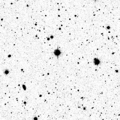
The initial processing of the data was accomplished in the same way as described in Paper I. This involved using the STARLINK CCDPACK reduction package to de-bias, flat-field, align and coadd the images. The reduced frames were then sky–subtracted (see Driver, Windhorst & Griffiths 1996) to remove any large–scale residual sky gradients – due mainly to internal scattered light from nearby bright stars and/or light leakage. Details of this subtracted sky background (mean signal in ADU and calibrated surface brightness) and its associated noise (in ADU) and 1 surface brightness limit can be found in columns 5–8 of Table 2. Figure 1 shows a greyscale plot of the final coadded and processed images obtained for A0868 and its associated field sight–line. Together, Table 2 and Figure 1 indicate that the data are of good quality and suitable for the purposes of our LD analysis (see Paper II). It is instructive to compare these images to the simulated data shown in Paper II, which were used to verify the technique we now apply in this paper.
3 Image detection and photometry
3.1 Generation of catalogues
The detection and photometry of objects within our CCD images was conducted automatically using the SExtractor software package (Bertin & Arnout 1996) in an identical manner to that described in Paper II. For this purpose a detection limit of mag arcsec-2 over 4 connected pixels together with the automated image de-blending algorithm were used; the magnitudes measured were Kron (1978) types taken within an aperture of radius = . Our measured magnitudes were corrected for Galactic extinction using values from the study of Burstein & Heiles (1982) and which are available for each cluster on NED222The NASA/IPAC Extra-galactic Database (NED) is operated by the Jet Propulsion Laboratory, California Institute of Technology, under contract with the National Aeronautics and Space Administration.; the actual values used are listed in Table 3. SExtractor utilises an Artificial Neural Network to perform star/galaxy separation and assigns a probability value to each object in the range 0 to 1 (where 1 indicates a perfectly stellar profile). Figure 2 shows a histogram of the star/galaxy likelihood values obtained for the entire data set. The peak at 0.95 represents the expected location of stellar objects and from this plot we choose to adopt a value of 0.90 as the critical division between stars and galaxies. Table 3 summarises the numbers of objects classified as stars in each field down to . The shaded area in Figure 2 shows the stellar likelihood for those objects with .
3.2 The non-cluster sight-lines
Figure 3 shows the individual galaxy counts (after star-galaxy separation and reddening correction) for each of the seven field sight-lines. The reference line is our optimal fit to the data of Metcalfe et al. (1995) and is given by over , and for . Incompleteness is indicated by the departure of our data from this reference line. In all cases other than the B2547 field, there is good qualitative agreement between our galaxy counts and those of Metcalfe et al. The apparent excess of galaxies in B2547 indicates the possibility of our sight-line in this case inadvertently passing through a nearby cluster. Examination of the image indicates an obvious excess of bright galaxies across this field. This, therefore, precludes us from using B2547 as a reference background field.
The middle panel of Figure 3 shows the mean galaxy counts constructed from all our field data (open circles) and with B2547 excluded (solid squares), minus the fit to the Metcalfe et al. data. This shows more quantitatively the good agreement between our data and those of Metcalfe et al. and indicates that our data our complete to beyond which our counts increasingly fall below the deeper Metcalfe et al. data. We adopt this value as our completeness limit. Note that in a number of the published papers on this topic a valiant effort has been made to push a little deeper by the application of isophotal correction methods. The problem with this approach is that it requires prior knowledge of the surface brightness distribution of the faint cluster populations, which is unknown. Here we have preferred to take the most conservative course of action which is to define our completeness limit as the magnitude at which the first sign of deviation between our field counts and the much deeper counts of Metcalfe et al. appear. In effect we are circumventing surface brightness selection effects by making a conservatively bright magnitude cut.
The bottom panel of Figure 3 illustrates the percentage variation of observed galaxies in each magnitude bin about the mean (as derived from all our field sight-lines except B2547). The symbols are as defined in the individual number-count plots at the top of Figure 3. The solid lines represent the anticipated variation in the counts from Poisson statistics. At bright magnitudes () the large variation (%) is a reflection of the limited size of our field of view ( arcminutes). At fainter magnitudes, down to our completeness limit , the variation seems slightly in excess of that expected from Poisson statistics. In particular, the counts in field B0868 lie systematically below the Poissonian limit. There could be several reasons for this: SExtractor incorrectly classifying galaxies as stars at the faintest limits, underestimation of the Galactic absorption in this relatively low galactic latitude field, or a genuine background inhomogeneity. Cross-referencing the different fields with their observational parameters in Table 1 indicates no obvious correlation, in this context, with seeing or airmass. The lack of a variation grossly in excess of the Poisson limits, on the other hand, suggests that it might well be valid to use the mean of all the field sight-lines (except B2547) for the background galaxy subtraction. The only exception here is at bright magnitudes () where it is clear that our data cover an insufficient field of view to constitute a fair comparison; this is further addressed in §4.2.
3.3 The cluster sight–lines
The image detection and photometry was performed for the cluster sight-lines using the same isophotal detection limit and detection parameters as for the field sight–lines. The resulting number counts from the seven cluster sight–lines are shown in Figure 4; again the optimal fit to the data of Metcalfe et al. (1995) is shown for reference purposes. In all cases the counts lie well above the reference line down to the limiting magnitude of , indicating the presence of a cluster. The lower panel shows the percentage excess of galaxies in each magnitude bin over the mean field counts. Apart from A0204 (our poorest cluster – see Table 1), all clusters show a significant excess at all magnitudes down to the detection limit. Comparison with Figure 3 indicates that this excess is significant.
In looking to establish here whether the form of the LD measured within each of our clusters is correlated in any way with global cluster properties (e.g. richness, BM–class), we have calculated from our data the mean local projected galaxy density – as formulated by Dressler (1980) – within each cluster field. This parameter, which we shall refer to as the Dressler density parameter (DDP), measures the projected density local to each galaxy by determining the area (in Mpc2) within which its 10 nearest neighbours with 333Equivalent to at the redshift of the clusters studied here, assuming km s-1 Mpc-1 are contained. Since Dressler showed the morphological (E/S0/Sp) mix of galaxies in rich clusters to be a strong and smoothly–varying function of this parameter, its consideration within this aspect of the study is clearly important. The mean DDP value evaluated for each cluster is listed in the column 7 of Table 1.
4 The luminosity distributions
4.1 Construction
The LD for each cluster was recovered via the statistical subtraction of the field galaxy counts from those observed towards the cluster. At bright magnitudes () this was accomplished using the field counts of Metcalfe et al. (1995). At fainter magnitudes () the counts measured in each cluster’s adjacent field region were used444Note that for A2547, the nearest acceptable field region, B0022, was used.. Star–galaxy separation was performed only at ; at fainter magnitudes it was assumed that each cluster’s comparison field sight-line had the same stellar surface density to the cluster sight-line. The rationale for using the Metcalfe et al. counts at bright magnitudes was because of their greater sky coverage and therefore better statistics at bright magnitudes. The use of our adjacent field counts at fainter magnitudes was to eliminate or minimize the following effects: (1) surface brightness–dependent systematics – both our cluster and adjacent field catalogues had the same surface brightness limit, (2) subtraction uncertainties due to large–scale structures, and (3) point spread function variations due to changing atmospheric conditions and/or detector aberrations.
As part of this process, an adjustment was made for the diminishing field of view available to fainter objects (see Paper I for full details). The apparent magnitude distributions derived for each cluster were converted to ones in absolute magnitude using the distance moduli listed in Table 1. To compute the distance moduli a standard flat cosmology (, , kms-1Mpc-1) was adopted and a uniform –band K-correction of (valid for ; Driver et al. 1994b) assumed. Figure 5 shows the final LDs (solid circles and errorbars) recovered for each of the seven clusters and also the mean LD for the entire ensemble. The latter was derived from a direct average of the individual LDs after normalising each distribution to unity. This ensures that the mean LD is not dominated by the richest cluster. Table 4 tabulates the data plotted in Fig. 5.
Qualitatively, Figure 5 suggests a wide variation in the recovered LDs in terms of their faint end () behaviour, ranging from the flat LD of A3888 to the steep LD of A0868. For reference, the solid line in Fig. 5 represents a flat () Schechter function (Schechter 1976). The larger errorbars for A0204 and A2547 illustrate the conclusions of Paper II, showing that the LD recovery technique eventually fails for poor clusters and this is due to the lack of contrast of the cluster against the background.
4.2 Evaluating the dwarf-to-giant ratios
Given the quality of the recovered LDs, and the intrinsic restrictions of using Schechter function fits (see Paper II), we elect to use a simpler and more versatile measure to quantify the LD’s, viz. the ratio of dwarfs () to giants ():
| (1) |
This approach was introduced by Ferguson & Sandage (1991) in their study of local poor groups and is also favoured by Secker & Harris (1996) in their analysis of the Coma cluster. In column 4 of Table 5 we list the DGR values derived from the LDs shown in Figure 5 and we see that they vary from 0.8 (A3888) to 3.1 (A0204), thus indicating an apparently large range in the dwarf component of these rich clusters. For those more familiar with Schechter function parameters, this equates to a faint–end slope variation of ; Fig. 6 shows the relation between and the DGR parameter if the cluster is assumed to be well described by a single Schechter function fit with . It is interesting to note that over bright absolute magnitudes () all clusters — with the possible exception of A2344 — exhibit similar LDs confirming the findings of Lumsden et al. (1997) of the universal nature of the bright end of the cluster LF. We also note that the cluster LDs do not conform to a strict Schechter function at bright magnitudes, but show a marginal excess indicative of the presence of a small population of overly luminous objects in cluster environments.
4.3 Robustness of the background subtraction
Paper II explored in detail the limitation of our photometric recovery technique and illustrated that the reliability of the recovered LD is a strong function of cluster richness, seeing and redshift, but relatively independent of LD shape. The critical step in the LD recovery process is the accuracy of the background subtraction which relies on the contrast of the cluster galaxy counts against those of the field. The most direct way of testing this accuracy with real data is to repeat the analysis using a different field reference sample. The methodology of the current recovery is based on the argument that an adjacent field sight-line is the most reliable reference and one which mitigates most concerns (accuracy of star/galaxy separation, background fluctuations etc). Nevertheless, it is arguable from Figure 3 that the variation in the individual field galaxy counts around the mean is sufficiently small that a subtraction based on the mean counts may be equally valid. To determine whether this small field–to–field variation has any significant effect on the results presented here, we reconstruct the LDs using a background subtraction based entirely on the mean counts over the full range of apparent magnitude (to compensate for the varying galactic latitudes we must now perform star/galaxy classification to our magnitude limit). The results are also shown in Figure 5 where they are overlaid on top of the original data points (solid circles) and plotted as open squares. In most cases the two data sets agree to within the specified errors. In two cases (A0868 & A2344) the differences are apparently systematic as opposed to random. These two clusters both lie close to the Galactic plane and the discrepancy may be a reflection of errors in the star-galaxy separation at fainter magnitudes. Despite the systematic trend in these two clusters, the broad shape of their LDs is consistent, both showing an upturn in their LDs regardless of which background subtraction is used. The over-riding qualitative impression from Figure 5 is the robustness of the results to the choice of background subtraction.
To quantify the dependence of our results on the background subtraction we recompute the DGR values based on this second reconstruction. These are shown in column 5 of Table 5 and can be compared to column 4 which shows the original values. In all cases the results agree to within their specified errors.
4.4 How accurately can we measure the DGR?
This question can be addressed using the mean cluster LD (see Fig. 5) which has a DGR of . Input parameters were assigned to our simulation software to produce a simulated f/3.3 AAT image for a cluster at z=0.15 with this same DGR value (and mean richness, c.f. Paper II). The simulated cluster was then put through the identical detection and photometric procedure as the real data and the final DGR value measured as for the real data. This procedure was repeated for 400 simulated clusters and field sight-lines. The resulting input and output DGR distributions are shown in Figure 7. The cross–hatched histogram represents the variation in the input distribution, with a mean DGR and standard deviation in a single measurement of (DGR) – this spread is because we only sample the central region of the simulated cluster image. The open histogram shows the recovered DGR distribution after image simulation, noise addition, detection, star-galaxy separation, image de-blending and final photometry (see Paper II). The recovered distribution is broader than the input distribution, as expected due to the process of simulation which introduces noise and object overlaps, and very slightly skewed to lower DGR (DGR and (DGR)). This series of simulations establishes firmly that the recovered DGR is a good representation of the input DGR and that the one-sigma measuring accuracy in the DGR is of the order .
4.5 Verification by simulation
To directly assess the reliability of the DGR measurements for each cluster, we undertook extensive Monte-Carlo simulations based on the method described in Paper II. We take as our starting point the parameters listed in Tables 1-5 and simulate eleven independent cluster and field sight-lines for each of our actual clusters. From these we derive the recovered DGRs after simulation, detection and analysis. Its worth noting that these simulations reflect both the statistical variances but also any systematic effects due to disparity between the field and cluster seeing and field and cluster noise limits etc. Figure 8 shows the resulting histograms of the recovered DGR and the final two columns of Table 5 shows the recovered mean DGR and its standard deviation. In almost all cases these values are less than the quoted errorbars, this is because throughout out error analysis we have assumed all data points in the LD are uncorrelated. These simulations underline the robustness of our results listed in Table 5.
It is also interesting to note that two of our clusters (A0204 and A2344) fall within the observational domain where reliable results are not guaranteed (see Paper II) and we can see that these clusters along with A2547 show the largest systematic errors and standard deviation errors in the recovered DGRs. Nevertheless these errors, derived via simulations, are smaller than those quoted in Column 4 & 5 of Table 5 and smaller than would be implied by Paper II555The actual GOF values for these simulations are: A0022=84%, A0204=72%, A0545=91%, A0868=95%, A2344=90% A2547=88% and A3888=74%. These is due to a number of reasons. The first is that the DGR is a less stringent test than Paper IIs Goodness-of-fit and while the DGR can be deemed reliable the exact LD distribution should be treated more cautiously. Secondly our actual data has substantially lower noise than that used in the earlier simulations of Paper II (our simulations had a 1- noise limit of 26 mags per sq arcsec compared to the numbers listed in column 8 of Table 2). The final reason is the general unreliability of the Abell richness classification (c.f Columns 4 and 7 of Table 1).
5 Discussion
As has already been highlighted in the previous section, the LDs we have derived and their associated DGRs show considerable variation across our sample. This raises a number of issues in relation to the universality of the LD, each of which we now address:
5.1 Is the data consistent with a ubiquitous cluster LD?
Having established via simulation the accuracy to which we can measure DGR values, we are in a position to assess whether those observed for the clusters in our sample are consistent with a universal LD for all cluster types. To address this, the distribution of observed DGR values is plotted as the solid histogram (scaled up by ) in Figure 7. The variation in the DGR value for the actual data has a mean666Note that the mean of the observed DGRs and the DGR of the mean LD are not expected to be identical of DGR, and a standard deviation of (DGR) which is inconsistent with our seven clusters having a ubiquitous parent LD at the level. We therefore consider it unlikely, based on our sample of seven clusters, that there exists a ubiquitous cluster LD and conclude that clusters are either: ‘normal’ ( DGR ), e.g. A0022, A0545, A2547; ‘dwarf-rich’ (DGR ), e.g. A0204, A0868, A2547 or ‘dwarf-poor’ (DGR ), e.g. A3888.
5.2 Is the DGR uniform throughout the cluster?
In Paper I we identified a luminosity–dependent segregation in A2554 in that the giant galaxies were more centrally concentrated than the dwarfs. If this is universal then we expect the DGRs to increase as a function of radius. Unfortunately the new data have a more limited coverage (typically 0.74 Mpc radius from cluster centre) than the A2554 data (1.40 Mpc), hence a full analysis of this segregation requires further data. However, we can make a preliminary investigation by measuring the DGRs for “inner” ( Mpc) and “outer” ( Mpc) regions of the clusters observed here; Table 5 shows the results. For clusters A0022 and A3888 the DGR values decrease in the outer regions contrary to the trend seen in A2554. For all other clusters the DGR increases significantly from the inner to outer region corroborating the trend seen in A2554. This further emphasises the fact that the LD and DGR observed within a cluster depends sensitively on over what physical region of the cluster the measurement is made. In this respect our data reveal two important trends: (1) significant variations in the DGR even over the limited radial limits ( Mpc) probed here, but also importantly (2) variations in the DGR from cluster to cluster are at a minimum within the central Mpc. Clearly further data need to be acquired to firm up these two results and these will be reported in future papers in this series.
5.3 Possible correlations between the DGR and cluster properties
Drawing upon the above results, Figure 9 shows the DGR values measured for the inner regions (top), the outer regions (middle), and the entire cluster (bottom), plotted against Bautz-Morgan class (Bautz & Morgan 1970), Abell richness and the mean DDP values derived for these regions. As noted in §5.2, there is less variation from cluster to cluster in the DGR observed in the inner regions and we see this graphically in the top panels of Figure 9 where the DGR values are mostly in agreement to within their uncertainties. For some reason, the balance between dwarf and giant galaxies appears to be similar within the inner cores ( Mpc) of clusters irrespective of their global properties. Taken at face value, this suggests some physical mechanism operating in the core of clusters between the giants and dwarfs. However, it is important to remember that it has not been established whether the dwarfs are actually in the core or are simply the projected density of a surrounding halo along the line-of-sight through the core.
In contrast to the inner regions, the outer regions do show trends, with the DGR exhibiting a reasonable correlation with BM–class and a strong anti–correlation with mean DDP. This is also reflected weakly in the “total” cluster plots shown in the bottom panels. In these outer regions, therefore, it is quite clear that either the dwarf galaxy population is diminished or the giant galaxy population is boosted in clusters where there is a higher overall local density of galaxies and which are dynamically more evolved (i.e. lower BM–class). The diminution of the dwarf population in this context is certainly consistent with the “galaxy harassment” scenario (Moore et al. 1996) which would predict that this process is most effective and has been in operation longer in the more relaxed and centrally dense clusters, thereby significantly whittling away their lower luminosity populations and hence reducing their DGR.
5.4 Is there a radial dependence? – A2554 revisited
All our new cluster LDs have substantially flatter faint–end slopes than that reported in recent publications, including our own (Driver et al. 1994a; Paper I; Wilson et al. 1997). Both the Driver et al. and Wilson et al. studies relied on isophotal corrections which are highly dependent on the assumed profiles for the fainter cluster members (Trentham 1998b). However, the more recent study of A2554 (Paper I) relied on no such correction which begs the question as to why A2554 shows a significantly higher DGR (DGR)? One possible reason, mentioned in §4.6, is the significantly larger areal coverage of the A2554 data ( Mpc cf Mpc for the seven clusters of this study). If the fainter galaxies are distributed more uniformally than the giants one might expect the DGR to increase with radius. To test this we reconstruct the DGR for A2554 as a function of radius. The results are shown in Figure 10 with the DGR being plotted both differentially (top panel) and cumulatively (bottom panel) as a function of radius. The vertical dashed line indicates the radial limit applicable to the 7 new clusters presented in this study. Both the cumulative and differential DGR show a marked increase as a function of radius, implying that for A2554 the dwarf population is more broadly distributed than the giants (see also Paper I). At a radius of 1 Mpc from the cluster centre the local DGR value is approximately 6-8 (comparable with a single Schechter function slope of ) as opposed to the central value of 3 ().
5.5 Decomposing the DGRs
Up until now we have considered only the DGR and have not explicitly examined the absolute numbers of giants and dwarfs within our clusters. In Figure 11, therefore, we plot the actual density of giants and dwarfs per Mpc2 for the inner and outer regions separately. For clarity the inner and outer giant points are linked by solid lines while the dwarf points are linked by dashed lines. The clusters are arranged from top to bottom in order of decreasing DDP with their Bautz-Morgan class denoted alongside. For the two densest clusters (A3888 & A0022) the dwarf galaxies actually exhibit a marginally steeper radial drop-off than for the giants. These two clusters are also low Bautz-Morgan types where spherical symmetry is more likely to be an accurate representation of the galaxy distribution and they are generally more relaxed. An additional concern is lensing. However Trentham (1998a) showed that lensing in the core region of a very rich cluster will enhance the background density by only %. For the remaining clusters, the dwarfs exhibit a significantly flatter radial drop-off and in three cases, A0545, A2547 & A0204, actually increases from the cluster centre – determined, of course, from the giant population. It is very difficult to understand how the density of dwarfs could possibly increase with respect to the inner region if the dwarfs exist in a smoothly distributed spherical profile around the primary cluster center777Since both the near-side and far-side outer dwarf populations would project onto the “inner” sight-line.. One intriguing possibility is that the core regions are devoid of dwarf galaxies, although why this should be the case for the poor rather than rich clusters is not clear. However, we note that these three clusters are all Bautz-Morgan class III and a second explanation is that in such clusters the dwarfs exhibit extremely asymmetrical profiles as might be expected in these non-relaxed environments. This asymmetry combined with a higher DGR in lower density environments would be sufficient to explain the observed increase.
6 Conclusions
We have recovered the luminosity distributions (from ) within the central regions ( Mpc) of seven clusters at . We find a variation in the recovered DGRs of 0.8—3.1 (equivalent to: ). This variation is found to be inconsistent at the 3 level with the notion of a universal cluster LD. However, we find that the LDs derived for the inner ( Mpc) core regions show more universality than those derived for the exterior ( Mpc) regions. The implication is that the clusters studied here show a wide range in the richness of their dwarf halos from very poor (DGR ) to extremely dwarf–rich (DGR ), equivalent to and respectively. Furthermore, there is a strong anti-correlation between the DGR and the mean local projected (Dressler) density in that clusters with lower overall projected densities contain a greater relative density of dwarf systems.
Re-analysis of earlier data on A2554 (see Paper I) re-confirms the strongly clustered nature of giant galaxies (), as opposed to the dwarf systems () for this cluster. Examining the densities of dwarf and giant galaxies independently in the inner and outer regions for our latest clusters suggests that for the densest and most relaxed clusters (i.e. Bautz-Morgan class I) the dwarfs, while seen in relatively fewer numbers, follow a similar density drop-off to the giants. Conversely, the lower density, dynamically unevolved clusters (i.e. Bautz-Morgan class III) exhibit an increase in their dwarf densities in the outer regions, suggesting that the dwarf-rich halos in these clusters are highly asymmetrical and extend well beyond the cluster radius surveyed (r Mpc as seen for A2554). This result, in conjunction with the general observed trend of higher relative density of dwarf to giant systems in less dense environments, implies a high density of dwarf systems in the field (see Marzke et al. 1994; Driver & Phillipps 1996).
The broad conclusion is that the distribution of dwarf galaxies does not necessarily follow that of the more luminous cluster members particularly for high Bautz-Morgan class clusters, implying an initial luminosity segregation and, more importantly, that the dwarfs have trod a separate evolutionary path than that of the giants. This segregation has already been predicted from the numerical models of Kauffmann et al. (1997). As we have previously discussed (§4.6), galaxy “harassment” may be a prime cause of this luminosity segregation due to the lower luminosity systems being the most susceptible to the strong tidal forces they encounter when entering a cluster (Moore et al. 1996). Further work is required – in particular, deep wide-field optical imaging – to determine how far the halo of dwarf galaxies around clusters extends and to quantify its possible contribution to the inferred dark matter halos of clusters (Navarro, Frenk & White 1996). Probing to higher redshifts will also establish whether the trends seen in the current sample evolve and may provide strong constraints to the evolutionary processes at work in rich clusters.
Speculatively then, the results presented here are consistent with a scenario in which clusters start from initially extended asymmetrical dwarf-rich environments and evolve towards fully relaxed giant rich clusters with severely diminished dwarf-poor halos. We note that remarkably similar results to those presented here have been found by Lôpez-Cruz (1997) based on an entirely independent study of northern Abell/ACO clusters.
Acknowledgments
The results presented here are based on observations made with the AAT and we thank the support and technical staff of the Anglo-Australian Observatory for their valuable assistance. We thank Stuart Ryder for riding the prime focus cage at the AAT during the January observations. SPD and WJC acknowledge the financial support of the Australian Research Council throughout this work. SP is supported by the Royal Society via a University Research Fellowship.
References
-
Abell G., 1958, ApJS, 3, 1.
-
Abell G., Corwin H.G., Olowin R., 1989, ApJS, 301, 83.
-
Abraham R.G., Tanvir N.R., Santiago B.X., Ellis R.S., Glazebrook K., van den Bergh S., 1996, MNRAS, L47
-
Barger A., Aragón-Salamanca A.S., Smail I., Ellis R.S., Couch W.J., Butcher H., Dressler A., Oemler A., Poggianti B.M., Sharples R.M., 1998, ApJ, in press
-
Bautz L.P., Morgan W.W., 1970; ApJ, 162, L149
-
Bernstein G.M., Nichol R.C., Tyson J.A., Ulmer M.P., Wittman D., 1995 AJ, 110, 1507
-
Bertin E., Arnout S., 1996, A&AS, 117, 393
-
Biviano A., Durret F., Gerbal D., Le Fèvre O., Lobo C., Mazure A., Slezak E., 1995, A&A, 297, 610
-
Burstein D., Heiles C., 1984, ApJS, 54, 33
-
Butcher H., Oemler A. Jr., 1978, ApJ, 219, 18
-
Charlot S., Silk J., 1994, 432, 453
-
Colless M., 1995, in Wide Field Spectroscopy and the Distant Universe, ed. S.J.Maddox & A.Aragon-Salamanca (Singapore: World Scientific), 263
-
Colless M., Dunn A.M., 1996, ApJ, 458, 435
-
Couch W.J., Ellis R.S., Sharples R.M., Smail I., 1994, ApJ, 430,121
-
Couch W.J., Barger A.J., Smail I., Ellis R.S., Sharples R.M., 1998, ApJ, 497, 188
-
De Propris, R., Pritchet, C.J., Harris, W.E., McClure, R.D., 1995, ApJ, 450, 534
-
De Propris, R., Pritchet, C.J., 1998, ApJ, submitted (astro-ph/9805281)
-
Dressler A., 1978, ApJ, 223, 765
-
Dressler A., 1980, ApJ, 236, 351
-
Dressler A., Oemler A. Jr., Butcher H.R., Gunn J.E., 1994, ApJ, 435, 23
-
Driver S.P., Phillipps S., Davies J.I., Morgan I., Disney M.J., 1994a, MNRAS, 268, 393.
-
Driver S.P., Phillipps S., Davies J.I., Morgan I., Disney M.J., 1994b, MNRAS, 266, 155
-
Driver S.P., Windhorst R.A., Griffiths R.E., 1995, ApJ, 453, 48
-
Driver S.P., Windhorst R.A., Ostrander E.J., Keel W.C., Griffiths R.E., Ratnatunga K.U., 1995, ApJL, 449, L23
-
Driver S.P., Phillipps, S., 1996, ApJ, 469, 529
-
Driver S.P., Couch W.J., Phillipps S., Windhorst R.A., 1996, ApJ, 466, L5
-
Driver S.P., Couch W.J., Phillipps S., Smith R.M., 1998, MNRAS, in press (Paper II)
-
Driver S.P., Couch W.J., Odewahn S.C., Windhorst R.A., 1997, in proc 18th Texas symp. on “Relativistic Astrophysics”, in press
-
Ellis R.S., Colless M., Broadhurst T.J., Heyl J., Glazebrook K., 1996, MNRAS, 280, 235
-
Ellis R.S., 1997, ARA&A, 35, 389
-
Ferguson H., Sandage A., 1991, AJ, 96, 1620
-
Godwin J., Peach J.V., 1977, MNRAS, 181, 323.
-
Graham J.A., 1982, PASP, 94, 244
-
Impey C., Bothun G.D., Malin D., 1988, ApJ, 330, 634
-
Kauffmann G., Nusser A., Steinmetz M., 1977, MNRAS, 286, 795
-
Koo D.C., Kron R.G., 1992, ARA&A, 30, 613
-
Kron R.G., 1978, PhD, Univ. Berkeley
-
Landolt A.U., 1992, AJ, 104, 1
-
Lilly S., Tresse L., Hammer F., Crampton D., Le Fèvre O., 1995, ApJ, 455, 108
-
Lobo C., Biviano A., Durret F., Gerbal D., Le Fèvre O., Mazure A., Slezak E., 1997, A&A, 317, 385
-
Lôpez-Cruz O., 1997, PhD, Univ. Toronto
-
Lôpez-Cruz O., Yee H.K.C., Brown J.P., Jones C., Forman W., 1997, ApJL, 475, 97
-
Lumsden S., Collins C.A., Nichol R.C., Eke V.R., Guzzo L., 1997, MNRAS, 290, 119
-
Marzke R., Huchra J.P., Geller M.J., 1994, ApJ, 428, 43
-
Metcalfe N., Shanks T., Fong R., Roche N., 1995, MNRAS, 273, 257
-
Moore B., Katz N., Lake G., Dressler A., Oemler A Jr., 1996, Nature, 379, 613
-
Moore B., Lake G., Katz N., 1998, ApJ, 495, 139
-
Navarro J.F., Frenk C.S., White S.D.M., 1996, ApJ, 462, 563
-
Oemler A. Jr., 1974, ApJ, 194, 1
-
Oemler A. Jr., Dressler A., Butcher H.R., 1997, ApJ, 474, 561
-
Phillipps S., Driver S.P., 1995, MNRAS, 274, 832
-
Phillipps S., Parker Q.A., Schwartzenberg J.M., Jones J.B., 1998, ApJ, 493, L59
-
Schade D.L., Barrientos F., Lôpez-Cruz O., 1997, 477, L17
-
Schechter P., 1976, ApJ, 203, 297
-
Secker J., 1996, ApJ, 469, 81
-
Secker J., Harris W.E., 1996, ApJ, 469, 623
-
Smail, I. Dressler A., Couch W.J., Ellis R.S., Oemler A.Jr., Butcher H., Sharples R.M., 1997, ApJS, 110, 213
-
Smith R.M., Driver S.P., Phillipps S., 1997, MNRAS, 287, 415 (Paper I)
-
Steidel C.C., Dickinson M., Persson S.E., 1994, ApJ, 437, L75
-
Thompson L.A., Gregory S.A., 1993, AJ, 106, 2197
-
Trentham N., 1997a, MNRAS, 286, 133
-
Trentham N., 1997b, MNRAS, 290, 334
-
Trentham N., 1998a, MNRAS, 295, 360
-
Trentham N., 1998b, MNRAS, 293, 71
-
Trèvese D., Crimele G., Appodia B., 1996, A & A, 315, 365
-
Wilson G., Smail I., Ellis R.S., Couch W.J., 1997, MNRAS, 284, 915
Tables
| Cluster | Abell | BM-type | FOV | DDP | ||
|---|---|---|---|---|---|---|
| Richness | (Mpc2) | (gals Mpc-2) | ||||
| A0022 | 0.143 | 39.85 | 3 | I | 1.53 | |
| A0204 | 0.156 | 40.09 | 1 | III | 1.75 | |
| A0545 | 0.154 | 40.06 | 4 | III | 1.72 | |
| A0868 | 0.153 | 40.04 | 3 | II-III | 1.70 | |
| A2344 | 0.145 | 39.91 | 1 | II | 1.56 | |
| A2547 | 0.149 | 39.98 | 2 | III | 1.64 | |
| A3888 | 0.168 | 40.27 | 2 | I-II | 1.96 |
1 Assuming H kms-1 Mpc-1 and .
| Field1 | Mean airmass | FWHM | Exp | Background | Noise | 1SBL3 | |
|---|---|---|---|---|---|---|---|
| (arcsec) | (min) | (ADU) | (mag arcsec-2) | (ADU) | (mag arcsec-2) | ||
| A0022 | 1.06 | 1.26 | 100 | 2578 | 21.0 | 12 | 26.8 |
| B0022 | 1.10 | 1.35 | 100 | 3197 | 20.7 | 14 | 26.6 |
| A0204 | 1.12 | 1.07 | 100 | 2689 | 21.0 | 13 | 26.8 |
| B0204 | 1.11 | 1.25 | 90 | 2423 | 20.9 | 11 | 26.8 |
| A0545 | 1.08 | 1.02 | 90 | 3266 | 20.52 | 21 | 25.9 |
| B0545 | 1.10 | 1.04 | 90 | 2234 | 20.9 | 13 | 26.5 |
| A0868 | 1.10 | 1.02 | 90 | 2523 | 20.7 | 13 | 26.5 |
| B0868 | 1.13 | 1.02 | 90 | 2317 | 20.8 | 14 | 26.4 |
| A2344 | 1.04 | 1.15 | 70 | 2732 | 20.9 | 19 | 26.3 |
| B2344 | 1.03 | 0.95 | 100 | 2726 | 20.9 | 10 | 27.0 |
| A2547 | 1.15 | 1.10 | 90 | 2453 | 20.9 | 17 | 26.3 |
| B2547 | 1.02 | 1.05 | 90 | 2216 | 21.0 | 9 | 27.0 |
| A3888 | 1.10 | 1.27 | 100 | 2987 | 21.1 | 19 | 26.3 |
| B3888 | 1.04 | 1.03 | 90 | 2338 | 21.1 | 14 | 26.7 |
1 A denotes the Abell cluster number and B the corresponding nearby field sight-line.
2 The brighter sky for A0545 is due to the setting moon resulting in a higher mean background and higher noise.
3 1SBL:- 1 surface brightness limit
| Cluster | Stars | l | b | ||
|---|---|---|---|---|---|
| ID | Cluster | Field | |||
| A0022 | 56 | 63 | 42.89 | -82.98 | 0.04 |
| A0204 | 58 | 43 | 148.09 | -67.83 | 0.06 |
| A0545 | 109 | 145 | 214.60 | -22.72 | 0.20 |
| A0868 | 138 | 116 | 244.72 | +32.49 | 0.03 |
| A2344 | 151 | 153 | 29.02 | -42.87 | 0.05 |
| A2547 | 48 | 63 | 42.14 | -66.13 | 0.03 |
| A3888 | 93 | 70 | 3.97 | -59.40 | 0.00 |
| MR | A0022 | A0204 | A0545 | A0868 | A2344 | A2547 | A3888 | A963 | A2554 | MEAN |
|---|---|---|---|---|---|---|---|---|---|---|
| Cluster | Giants | Dwarfs | Dwarf-to-Giant ratios | ||||
|---|---|---|---|---|---|---|---|
| Name | Final | Alternate | Mpc | Mpc | Simulated | ||
| A0022 | |||||||
| A0204 | |||||||
| A0545 | |||||||
| A0868 | |||||||
| A2344 | |||||||
| A2547 | |||||||
| A3888 | |||||||
![[Uncaptioned image]](/html/astro-ph/9809206/assets/x1.png)


.


